fixed-effects parameters, the estimated covariance components, and the estimated .... Maximum likelihood (ML) was used to obtain the parameter estimates of.
Web Appendix to ‘Estimating the reliability of repeatedly measured endpoints based on linear mixed-effects models. A tutorial’ Wim Van der Elst, Geert Molenberghs, Dieter Hilgers, Geert Verbeke, & Nicole Heussen This Web Appendix contains six main parts. In Part I, the Delta method-based 95% CIs of the estimated b for ZSV (the outcome that was considered in the case study in Van der Elst et al., reliability coefficients ( R) 2016) are provided. In Part II (starting on page 3), a sensitivity analysis is conducted where the impact of 2 clinically deviating animals on the results is examined. In Part III (starting on page 6), a sensitivity analysis is conducted where the impact of using a different fixed-effect structure of the model (i.e., using different covariates) on the results is examined. In Part IV (starting on page 8), the use of the newly developed R package CorrMixed (estimate Correlations based on linear Mixed-effect models) is illustrated. In Part V (starting on page 21), it is detailed how the main reliability analyses can be conducted in SAS. In Part VI b Finally, (starting on page 29), details are provided on the computation of the Delta method-based CIs for R. in Part VII (starting on page 30), a residual analysis is conducted and the extent to which particular animals exert a strong influence on the results (i.e., the restricted likelihood distances of the models, the estimated fixed-effects parameters, the estimated covariance components, and the estimated reliability coefficients) is evaluated.
1
Part I
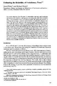
b in Bootstrap- and Delta method-based CIs for R the case study b for ZSV were based on a nonIn Van der Elst et al. (2016), the CIs of the estimated reliability coefficients ( R) parametric bootstrap procedure. Alternatively, these CIs can be computed based on the Delta method (see also Part VI of this Web Appendix, starting on page 29). Figure 1 shows the Delta method- (black dashed lines) and bootstrap-based (blue dashed lines) 95% CIs b (black solid line) for ZSV based on Model 1 (left figure) and 2 (right figure). As can be seen, around R the Delta method- and bootstrap-based CIs largely overlapped – and it can thus be concluded that both methods yielded similar results.
1.0
Model 2
1.0
Model 1
0.0
Reliability
0.5
Delta method Bootstrap
−0.5
−0.5
0.0
Reliability
0.5
Delta method Bootstrap
0
10
20
30
40
0
Time of measurement
10
20
30
40
Time lag
b for ZSV based on Model 1 (left figure) and Model Figure 1: Delta method- and bootstrap-based 95% CIs of R 2 (right figure).
2
Part II
Sensitivity analysis: two clinically deviating animals In Van der Elst et al. (2016), the reliability of the ZSV outcome was estimated based on the data of all 12 available animals. However, based on clinical considerations, it could be argued that 2 of the animals differed from the rest of the group. To evaluate the impact of these 2 deviating animals on the results (i.e., the estimated R and their CIs), the data were re-analyzed excluding these 2 animals (sensitivity analysis). Figures 2 and 3 show the estimated R and their 95% CIs based on analyses that used all available data (N = 12) and a subset of the data that excluded the 2 clinically deviating animals. Figure 2 shows the results � � b t1 , t j and R b t20 , t j (not all based on Models 1 and 2. Figure 3 shows the results based on Model 3 for R � b tk , t j are shown to avoid cluttered figures). As can be seen, the estimated R were slightly higher when R the 2 clinically deviating animals were excluded from the analyses – though the estimates were very similar and it can thus be concluded that the results were not substantially affected by these 2 clinically deviating animals.
3
0.5 Reliability 0.0 −0.5
−0.5
0.0
Reliability
0.5
1.0
Model 1, N=2 excluded
1.0
Model 1, all data
20
30
40
0
10
20
30
Time of measurement
Time of measurement
Model 2, all data
Model 2, N=2 excluded
40
0.5 −0.5
0.0
Reliability −0.5
0.0
Reliability
0.5
1.0
10
1.0
0
0
10
20
30
40
0
Time of measurement
10
20
30
40
Time of measurement
Figure 2: Estimated reliabilities (solid lines) and 95% bootstrap-based Confidence Intervals (dashed lines) for ZSV based on Model 1 (top) and Model 2 (bottom) using all data (left) and excluding 2 clinically deviating animals (right) from the analyses.
4
0.5 20
30
40
0
10
20
30
Time of measurement
Time of measurement
Estimated R(t20, tj), all data
Estimated R(t20, tj), N=2 excluded
40
0.5 0.0 −0.5 −1.0
−1.0
−0.5
0.0
Reliability
0.5
1.0
10
1.0
0
Reliability
0.0
Reliability
−1.0
−0.5
0.0 −1.0
−0.5
Reliability
0.5
1.0
Estimated R(t1, tj), N=2 excluded
1.0
Estimated R(t1, tj), all data
0
10
20
30
40
0
Time of measurement
10
20
30
40
Time of measurement
� � b t1 , t j and R b t20 , t j (solid lines) and 95% bootstrap-based Confidence Intervals (dashed lines) Figure 3: R for ZSV based on Model 3 using all data (left) and excluding 2 clinically deviating animals (right) from the analyses.
5
Part III
Sensitivity analysis: fixed-effect structure of the models In Van der Elst et al. (2016), the reliability of the ZSV outcome was estimated based on three models which had a different random-effect structure and an identical fixed-effect structure. In particular, all models included PEEP (coded with 5 dummies), cycle (coded with 3 dummies) and measurement moment (coded as a fractional polynomial of order M = 3, i.e., β 1 t2 + β 2 t2 log(t) + β 3 t3 with t = measurement moment) in the fixed-effect part. The models that include all covariates are referred to as the ‘full’ Models 1–3. The question may arise whether the results are sensitive to the fixed-effect structure of the model. To evaluate this, the non-significant covariates (using α = 0.05) were excluded from the models based on a series of likelihood ratio tests. Maximum likelihood (ML) was used to obtain the parameter estimates of these models (rather than Restricted Maximum Likelihood), because valid classical likelihood ratio tests for the mean structure of nested models can only be achieved with ML inference (Verbeke & Molenberghs (2000)). The models that only include the significant covariates are referred to as the ‘reduced’ Models 1–3. The sensitivity of the results for the mean structure of the model can subsequently be evaluated by comparing the reliability estimates that are obtained based on the full and the reduced Models 1–3. Results of the analyses Using likelihood ratio tests (data not shown), it was established that the reduced Model 1 only included PEEP in the mean structure of the model. The reduced Model 2 was identical to the full model (i.e., all covariates in the full model were significant). The reduced Model 3 included Cycle and PEEP. Figure 4 shows the estimated reliability coefficients based on the fitted full (left figures) and reduced (right figures) Models 1 (top figures) and 3 (bottom figures) results. No results are shown for Model 2 because the full and the reduced model were identical. As can be seen, the results for the full and the b = 0.441 (with 95% Confidence Interval reduced Models 1 and 3 were similar. For example, for Model 1, R b [0.198; 0.618]) based on the full model and R = 0.438 (with 95% Confidence Interval [0.180; 0.600]) based on the reduced model. The results of the analyses thus indicate that the estimated reliabilities are not strongly affected by the fixed-effect specification of the model (provided that the mean structure of the model is supported by the data).
6
0.5 Reliability 0.0 −0.5
−0.5
0.0
Reliability
0.5
1.0
Model 1, reduced fixed−effects structure
1.0
Model 1, full fixed−effects structure
10
20
30
40
0
10
20
30
40
Time of measurement
Model 3, full fixed−effects structure
Model 3, reduced fixed−effects structure
0.5 Reliability 0.0 −0.5
−0.5
0.0
Reliability
0.5
1.0
Time of measurement
1.0
0
0
10
20
30
40
0
Time of measurement
10
20
30
40
Time of measurement
Figure 4: Estimated reliabilities (solid lines) and 95% bootstrap-based Confidence Intervals (dashed lines) for ZSV based on the ‘full’ (left figures) and the ‘reduced’ (right figures) Model 1 (top figures) and Model 3 (bottom figures) results. The reliability estimates based on Model 3 do not include confidence intervals to avoid cluttered figures.
7
Part IV
R-based reliability analyses In this Part, it will be illustrated how the Linear Mixed Model (LMM)-based approach to estimate reliability (for details, see Van der Elst et al., 2016) can be carried-out in practice using the R package CorrMixed. In Van der Elst et al. (2016), the data of Pikkemaat et al. (2014) were analyzed. The data of the case study are not in the public domain so they cannot be freely distributed. As an alternative, the data of a hypothetical study that has the same formal characteristics as the Pikkemaat et al. (2014) study (i.e., the same number of animals, similar correlation structures in the data, etc.) will be analyzed here. Obviously, since we are using data that are similar but different from the data analyzed in Van der Elst et al. (2016), the results will also differ.
1
The dataset
The data of the fictitious study are included in the R package CorrMixed and they can be downloaded in .txt format via https://dl.dropboxusercontent.com/u/8416806/Example.Data_Library.txt (for use in e.g., SAS). R is a free software package for statistical analysis that can be downloaded via http://www. r-project.org/. The dataset contains 360 observations on 5 variables: • Id: the animal identifier. There are 10 animals in the dataset. • Cycle: similarly to what was the case in the Pikkemaat et al. (2014) study, the same experiment is repeated multiple times in the same animal. Cycle refers to the nth repetition of the experiment (min. = 1, max. = 4). • Condition: the experimental condition under which the outcome was measured. There are at most 16 experimental conditions within a cycle (similar to the different levels of PEEP in the Pikkemaat et al., 2014 study). • Time: the time point at which the outcome was measured (min. = 1, max. = 47). It is assumed that the time between two successive measurement moments is the same. • Outcome: a continuous outcome. The data are in the ‘long’ format, which means that there are multiple rows for each animal, i.e., one row for each time the outcome was measured. For example, the first three rows in the data file look like this: Id 1 1 1 ...
Cycle 1 1 1 ...
Condition 1 2 3 ...
Time 1 2 3 ...
Outcome 117.554 113.738 108.160 ...
After installation of the CorrMixed package in R (using the install.packages(’CorrMixed’) command; note that R is case-sensitive), the following code is used to load the package into memory: library(CorrMixed) The data of the (fictitious) case study are loaded using the command:
8
data(Example.Data) Example.Data[1:5,] ## ## ## ## ## ##
2
# load the data # have a look at the first five data rows
Id Cycle Condition Time Outcome 1 1 1 1 117.544003 1 1 2 2 113.738338 1 1 3 3 108.159814 1 1 4 4 91.962801 1 1 5 5 67.601301
1 2 3 4 5
Exploratory data analysis
A plot of the individual profiles for all animals and the mean evolution over time can be obtained using the Spaghetti.Plot() function of the CorrMixed package. This function requires the following arguments: • Dataset= : the name of the dataset. • Outcome=, Id=, Time= : the names of the outcome, subject indicator (Id) and time variable. By default, the individual profiles and the overall mean are provided. The following command can be used to obtain a spaghetti plot for the case study data:
100 0
50
Outcome
150
200
250
Spaghetti.Plot(Dataset=Example.Data, Outcome="Outcome", Id="Id", Time="Time")
0
10
20
30
40
Time
Other options are possible, for example, a plot that shows the median (rather than the mean) and no individual profiles can be requested using the command: Spaghetti.Plot(Dataset=Example.Data, Outcome="Outcome", Id="Id", Time="Time", Add.Profiles=FALSE, Add.Mean=FALSE, Add.Median=TRUE)
9
250 200 150 100 0
50
Outcome
0
10
20
30
40
Time
Fractional polynomials As was also the case with the ZSV outcome, the plots indicate that the relation between time and the outcome is quite complex and cannot be modeled in a straightforward way by using e.g., linear or quadratic polynomials. Therefore, fractional polynomials will be considered. The function Fract.Poly (Fractional Polynomials) of the CorrMixed package is useful in this respect. It requires the following arguments: • Covariate=, Outcome=, Dataset= : the names of the covariate, outcome, and dataset. • S=: the set that specifies the powers that will be considered in the different models. By default, S = {−2, −1, −0.5, 0, 0.4, 1, 2, 3}. • Max.M=: the maximum order to be considered for the fractional polynomials. Here, we request an analysis using the standard set S and m = 3, i.e., fractional polynomials of order 1, 2, and 3 will be considered: FP