web-based animation of geometric algorithms

WEB-BASED ANIMATION OF GEOMETRIC ALGORITHMS

Alejo Hausner

A DISSERTATION PRESENTED TO THE FACULTY OF PRINCETON UNIVERSITY IN CANDIDACY FOR THE DEGREE OF DOCTOR OF PHILOSOPHY

November 2001

c Copyright by Alejo Hausner 2001 All Rights Reserved

ii

Abstract This thesis looks at animation as a means of explaining software and algorithms, and considers human and computer factors that come into play. Understanding software is critical, because it enters so many aspects of our lives. Of course, students need to learn algorithms and programming techniques, but even experienced practicioners find that aspects of the programs they have written can exceed their understanding. For this reason, explanatory tools are sorely needed. By considering the types of uses that algorithm animation may be put to, we establish that it resembles visual arts, but, just as importantly, that there is little hope for automatic systems that can produce a useful animation based on a pseudocode description of an algorithm. Animation demands human guidance. Hence a good AA system must be interactive, and we establish a thorough list of requirements for such a system. We propose a portable web-based system. One important requirement is that algorithms and animations must run as separate processes. This separation yields many benefits, including robustness, repeatable algorithm runs, and reversible animation, although it necessitates extra effort to overcome the loss of immediacy that the audience might experience. To test this and other requirements, we implemented a Java-based system and animated many algorithms for it. The system is general, although it has features to ease animation of geometric algorithms in particular. It has been used to create successful web pages and video recordings.

iii

Acknowledgements This thesis would not have been possible without the kind guidance of my supervisor, David Dobkin. His patience and generosity are greatly appreciated. He was always available to discuss and share his extensive expertise, and his relaxed manner helped ease my frazzled nerves on many occasions. I also want to thank my thesis readers, Bernard Chazelle and Tom Funkhouser, both of whom suggested that software visualization can indeed aid the process of debugging. Emden Gansner served as an enthusiastic user of my software, and helped to isolate many bugs. Ayelet Tal was the one who originally pointed out the challenge of mid-execution interaction. My office mate Emil Praun not only introduced me to Inventor, but was a true friend. John Hainsworth suggested named color mappings. Last and not least, I want to thank my wife Leslie, who endured many long hours correcting logical lapses and otherwise helped me enormously with the proofreading. This work was funded in part by the NSF, under grants CCR-96-23768, CCR96-43913 and CCR-97-31535, and by the U.S. Army Research Office, under grant DAAH04-96-1-0181. Their support is gratefully acknowledged.

iv

Contents Abstract

iii

Acknowledgements

iv

1 Introduction

1

1.1

The Problem . . . . . . . . . . . . . . . . . . . . . . . . . . . . . . .

1

1.2

A Way Out . . . . . . . . . . . . . . . . . . . . . . . . . . . . . . . .

2

1.2.1

Algorithm Animation . . . . . . . . . . . . . . . . . . . . . . .

2

1.3

No Script . . . . . . . . . . . . . . . . . . . . . . . . . . . . . . . . .

4

1.4

Events . . . . . . . . . . . . . . . . . . . . . . . . . . . . . . . . . . .

4

1.5

Challenges . . . . . . . . . . . . . . . . . . . . . . . . . . . . . . . . .

6

1.5.1

The Audience . . . . . . . . . . . . . . . . . . . . . . . . . . .

6

1.5.2

Visualization is Difficult . . . . . . . . . . . . . . . . . . . . .

7

1.5.3

Animation is Difficult . . . . . . . . . . . . . . . . . . . . . . .

10

1.6

Benefits . . . . . . . . . . . . . . . . . . . . . . . . . . . . . . . . . .

11

1.7

Thesis Contributions . . . . . . . . . . . . . . . . . . . . . . . . . . .

12

2 Previous Work 2.1

2.2

15

General systems . . . . . . . . . . . . . . . . . . . . . . . . . . . . . .

16

2.1.1

Sorting out Sorting . . . . . . . . . . . . . . . . . . . . . . . .

16

2.1.2

BALSA and Zeus . . . . . . . . . . . . . . . . . . . . . . . . .

16

2.1.3

“Descendants” of BALSA . . . . . . . . . . . . . . . . . . . .

20

Geometry-oriented Systems . . . . . . . . . . . . . . . . . . . . . . .

25

2.2.1

25

Two-dimensional Systems . . . . . . . . . . . . . . . . . . . . v

2.3

2.2.2

Beyond Two Dimensions . . . . . . . . . . . . . . . . . . . . .

27

2.2.3

Mocha . . . . . . . . . . . . . . . . . . . . . . . . . . . . . . .

30

Visualizations . . . . . . . . . . . . . . . . . . . . . . . . . . . . . . .

32

2.3.1

Mathematical Visualization . . . . . . . . . . . . . . . . . . .

32

2.3.2

Demonstrations . . . . . . . . . . . . . . . . . . . . . . . . . .

34

2.3.3

Algorithm Animations . . . . . . . . . . . . . . . . . . . . . .

34

2.3.4

Interactive Visualizations . . . . . . . . . . . . . . . . . . . . .

38

3 Theoretical Considerations 3.1

3.2

3.3

3.4

41

Technological Maturation . . . . . . . . . . . . . . . . . . . . . . . .

44

3.1.1

Explanation vs. Entertainment . . . . . . . . . . . . . . . . .

44

3.1.2

Historical Parallels . . . . . . . . . . . . . . . . . . . . . . . .

45

Uses of Algorithm Animation . . . . . . . . . . . . . . . . . . . . . .

48

3.2.1

Algorithm Design: Rapid Prototyping

. . . . . . . . . . . . .

49

3.2.2

Implementation: Debugging . . . . . . . . . . . . . . . . . . .

49

3.2.3

Communication . . . . . . . . . . . . . . . . . . . . . . . . . .

50

Requirements . . . . . . . . . . . . . . . . . . . . . . . . . . . . . . .

52

3.3.1

The Need for Visualization . . . . . . . . . . . . . . . . . . . .

52

3.3.2

The Need for Interactivity . . . . . . . . . . . . . . . . . . . .

57

3.3.3

The Need for a Programming Environment . . . . . . . . . . .

61

3.3.4

Automatic Animation . . . . . . . . . . . . . . . . . . . . . .

66

3.3.5

Who benefits? . . . . . . . . . . . . . . . . . . . . . . . . . . .

68

Summary . . . . . . . . . . . . . . . . . . . . . . . . . . . . . . . . .

69

4 Requirements 4.1 4.2

73

Events . . . . . . . . . . . . . . . . . . . . . . . . . . . . . . . . . . .

74

4.1.1

Deferred Graphics . . . . . . . . . . . . . . . . . . . . . . . . .

74

Run Modes . . . . . . . . . . . . . . . . . . . . . . . . . . . . . . . .

78

4.2.1

Asynchronous Run Mode . . . . . . . . . . . . . . . . . . . . .

79

4.2.2

Synchronous Run Mode . . . . . . . . . . . . . . . . . . . . .

81

4.2.3

Immediate Run Mode . . . . . . . . . . . . . . . . . . . . . .

82

4.2.4

Hybrid Modes . . . . . . . . . . . . . . . . . . . . . . . . . . .

82

vi

4.3

4.4 4.5

4.6

4.7

4.8

4.9

Composite Events . . . . . . . . . . . . . . . . . . . . . . . . . . . . .

83

4.3.1

Parallel Events . . . . . . . . . . . . . . . . . . . . . . . . . .

83

4.3.2

Nested Events . . . . . . . . . . . . . . . . . . . . . . . . . . .

83

Inputs . . . . . . . . . . . . . . . . . . . . . . . . . . . . . . . . . . .

85

4.4.1

Programmatic Input . . . . . . . . . . . . . . . . . . . . . . .

85

Interaction . . . . . . . . . . . . . . . . . . . . . . . . . . . . . . . . .

87

4.5.1

Debugger Integration . . . . . . . . . . . . . . . . . . . . . . .

89

4.5.2

Gesture Translation . . . . . . . . . . . . . . . . . . . . . . . .

90

4.5.3

Before-and-After . . . . . . . . . . . . . . . . . . . . . . . . .

91

4.5.4

Data Modelers . . . . . . . . . . . . . . . . . . . . . . . . . .

92

4.5.5

Interaction and Run Mode . . . . . . . . . . . . . . . . . . . .

93

Time Control . . . . . . . . . . . . . . . . . . . . . . . . . . . . . . .

94

4.6.1

Waypoints . . . . . . . . . . . . . . . . . . . . . . . . . . . . .

94

4.6.2

Rewinding . . . . . . . . . . . . . . . . . . . . . . . . . . . . .

95

4.6.3

Gradual Changes . . . . . . . . . . . . . . . . . . . . . . . . .

95

4.6.4

Semantic Zooming . . . . . . . . . . . . . . . . . . . . . . . .

96

Abstraction and Tags . . . . . . . . . . . . . . . . . . . . . . . . . . .

97

4.7.1

Preserving Symbolic Information . . . . . . . . . . . . . . . .

98

4.7.2

Attribute Tags . . . . . . . . . . . . . . . . . . . . . . . . . .

99

4.7.3

Object Tags . . . . . . . . . . . . . . . . . . . . . . . . . . . .

99

4.7.4

Event Tags . . . . . . . . . . . . . . . . . . . . . . . . . . . . 100

Multimedia . . . . . . . . . . . . . . . . . . . . . . . . . . . . . . . . 101 4.8.1

Web Pages . . . . . . . . . . . . . . . . . . . . . . . . . . . . . 102

4.8.2

Device Dependence . . . . . . . . . . . . . . . . . . . . . . . . 102

4.8.3

Video Timing . . . . . . . . . . . . . . . . . . . . . . . . . . . 104

4.8.4

Camera Control . . . . . . . . . . . . . . . . . . . . . . . . . . 105

Event Styles . . . . . . . . . . . . . . . . . . . . . . . . . . . . . . . . 106 4.9.1

Style List . . . . . . . . . . . . . . . . . . . . . . . . . . . . . 106

4.9.2

Style Coverage . . . . . . . . . . . . . . . . . . . . . . . . . . 107

4.10 Summary . . . . . . . . . . . . . . . . . . . . . . . . . . . . . . . . . 108

vii

5 Design and Implementation 5.1

5.2

5.3

111

Design . . . . . . . . . . . . . . . . . . . . . . . . . . . . . . . . . . . 112 5.1.1

Goals . . . . . . . . . . . . . . . . . . . . . . . . . . . . . . . . 112

5.1.2

Consequences . . . . . . . . . . . . . . . . . . . . . . . . . . . 113

5.1.3

Omissions . . . . . . . . . . . . . . . . . . . . . . . . . . . . . 114

Implementation . . . . . . . . . . . . . . . . . . . . . . . . . . . . . . 116 5.2.1

Execution Modes . . . . . . . . . . . . . . . . . . . . . . . . . 117

5.2.2

Input Generators . . . . . . . . . . . . . . . . . . . . . . . . . 117

5.2.3

Algorithms . . . . . . . . . . . . . . . . . . . . . . . . . . . . 118

5.2.4

Renderers . . . . . . . . . . . . . . . . . . . . . . . . . . . . . 121

5.2.5

Event History . . . . . . . . . . . . . . . . . . . . . . . . . . . 122

5.2.6

Color Mappings . . . . . . . . . . . . . . . . . . . . . . . . . . 124

5.2.7

Event Player

5.2.8

3D Window . . . . . . . . . . . . . . . . . . . . . . . . . . . . 127

5.2.9

External Renderer . . . . . . . . . . . . . . . . . . . . . . . . 132

. . . . . . . . . . . . . . . . . . . . . . . . . . . 125

Summary . . . . . . . . . . . . . . . . . . . . . . . . . . . . . . . . . 133

6 Results

134

6.1

Products . . . . . . . . . . . . . . . . . . . . . . . . . . . . . . . . . . 135

6.2

Performance . . . . . . . . . . . . . . . . . . . . . . . . . . . . . . . . 135

6.3

Web pages . . . . . . . . . . . . . . . . . . . . . . . . . . . . . . . . . 136

6.4

Videos . . . . . . . . . . . . . . . . . . . . . . . . . . . . . . . . . . . 140

6.5

6.6

6.4.1

SOCG’98 . . . . . . . . . . . . . . . . . . . . . . . . . . . . . 140

6.4.2

SOCG’99 . . . . . . . . . . . . . . . . . . . . . . . . . . . . . 142

Results . . . . . . . . . . . . . . . . . . . . . . . . . . . . . . . . . . . 146 6.5.1

Human Issues . . . . . . . . . . . . . . . . . . . . . . . . . . . 146

6.5.2

Reversibility and Playback . . . . . . . . . . . . . . . . . . . . 147

6.5.3

Discontinuity Values . . . . . . . . . . . . . . . . . . . . . . . 150

6.5.4

Gradual vs Discrete Changes . . . . . . . . . . . . . . . . . . . 151

Obstacles to Debugging . . . . . . . . . . . . . . . . . . . . . . . . . . 152 6.6.1

Focused queries . . . . . . . . . . . . . . . . . . . . . . . . . . 154

viii

6.7

6.8

6.6.2

Program vs. Algorithm . . . . . . . . . . . . . . . . . . . . . . 154

6.6.3

Secondary Data Structures . . . . . . . . . . . . . . . . . . . . 155

Loss of Information . . . . . . . . . . . . . . . . . . . . . . . . . . . . 156 6.7.1

Compilation . . . . . . . . . . . . . . . . . . . . . . . . . . . . 156

6.7.2

Loss through Animation . . . . . . . . . . . . . . . . . . . . . 157

6.7.3

Root Cause . . . . . . . . . . . . . . . . . . . . . . . . . . . . 159

Successes . . . . . . . . . . . . . . . . . . . . . . . . . . . . . . . . . . 159

7 Summary and Conclusion

160

7.1

Summary . . . . . . . . . . . . . . . . . . . . . . . . . . . . . . . . . 160

7.2

Open Problems . . . . . . . . . . . . . . . . . . . . . . . . . . . . . . 161

7.3

Future Prospects . . . . . . . . . . . . . . . . . . . . . . . . . . . . . 161 7.3.1

Discontinuity Values . . . . . . . . . . . . . . . . . . . . . . . 162

7.3.2

3D Polygon Sorting . . . . . . . . . . . . . . . . . . . . . . . . 162

7.3.3

Video Distribution . . . . . . . . . . . . . . . . . . . . . . . . 163

7.3.4

Composite Data Structures . . . . . . . . . . . . . . . . . . . 163

7.3.5

Graph Layout . . . . . . . . . . . . . . . . . . . . . . . . . . . 164

7.3.6

Indirection . . . . . . . . . . . . . . . . . . . . . . . . . . . . . 164

7.3.7

Conclusion . . . . . . . . . . . . . . . . . . . . . . . . . . . . . 165

ix

List of Figures 1

Four stages a quicksort animation. a: initial array, b: intial partition, c: first recursion, d: sorted array. The algorithm implementation obviously has a bug. . . . . . . . . . . . . . . . . . . . . . . . . . . .

3

2

Four views of an array of numbers, before and after sorting. . . . . .

8

3

Balanced and unbalanced binary search trees . . . . . . . . . . . . . .

8

4

Two drawings of the same graph. Figure a shows that the graph is complete, while b shows that it is planar. . . . . . . . . . . . . . . . .

9

5

Graphs with symmetric structures. a: complete. b: bipartite. . . . . .

9

6

A snapshot from the final race in “Sorting Out Sorting”. Quicksort is winning the race. . . . . . . . . . . . . . . . . . . . . . . . . . . . . .

7

A screen from BALSA-II, showing the first-fit binpacking algorithm. The two views show the results of using random or sorted data. . . .

8

17 19

Zeus: an Animation of Selection Sort. In one control panel, the user has set the relative costs of swaps and comparisons, and in another the input generator determines the initial data. Two views show the algorithm state as plots of sticks and dots. . . . . . . . . . . . . . . .

9

A screen image from AnimA, showing the many algorithms implemented on the system

10

21

. . . . . . . . . . . . . . . . . . . . . . . . . .

22

A snapshot of Tango on X-Windows, running the first-fit bin packing algorithm. An object of size 5 is being tested for fit into the second bin. 23

11

A race between insertion sort and quick-sort, produced by Stills . . .

12

A snapshot from the Workbench for Compuational Geometry, showing a visibility algorithm on a triangulated polygon. . . . . . . . . . . . . x

24 27

13

A snapshot from Geobench, showing a sweepline algorithm for the Voronoi diagram of points on the plane. . . . . . . . . . . . . . . . . .

14

Geomview in action, showing the approximate convex hull of points in convex position. . . . . . . . . . . . . . . . . . . . . . . . . . . . . . .

15

28 29

A snapshot from GASP, showing an object that cannot be taken apart with two hands using only translations. . . . . . . . . . . . . . . . . .

31

16

A sphere is smoothly turned inside-out, from the film “Outside In”. .

33

17

A still from “Optimal Two-Dimensional Triangulations”. The polygonal outline of the USA is being triangulated. Lighter triangles have larger minimum angles. . . . . . . . . . . . . . . . . . . . . . . . . . .

35

18

A still from “Boolean Formulae for Simple Polygons” . . . . . . . . .

35

19

A still from “The New Jersey Line-Segment-Saw Massacre” . . . . . .

36

20

A still from “Building and Using Polyhedral Hierarchies” . . . . . . .

37

21

A still from “An Animation of a Fixed-Radius All-Nearest Neighbors Algorithm” . . . . . . . . . . . . . . . . . . . . . . . . . . . . . . . .

22

38

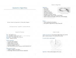
A still from “Visualizing Fortune’s Sweepline Algorithm for Planar Voronoi Diagrams”. We can see the sweepline, the parabolic fronts, and the partially constructed Voronoi Diagram. . . . . . . . . . . . .

23

39

A still from “Exact Collision Detection for Interactive Environments”. Look carefully, and you will see that only objects whose bounding boxes overlap (the cube and the fingers) trigger distance calculations (the lines from the fingers to the cube face). . . . . . . . . . . . . . .

24

40

Evidence of maturating use of perspective: a) Perugino, “The Delivery of the Keys”: perspective as conspicuous spectacle. b) Pieter de Hooch, “The Bedroom”: perspective as inconspicuous tool. . . . . . . . . . .

25

45

Popular conception of computers, then and now: a) A machine room with whirling tape drives. b) A web browser. . . . . . . . . . . . . . .

46

26

Fortune’s sweep: The implementation fails on degenerate inputs . . .

50

27

A buggy version of bubble-sort: animation finds an off-by-one bug . .

51

28

The properties of the Fresnel integral (c) can be conveyed as tables of numbers (a) or, more expressively, as a graph (b). . . . . . . . . . . . xi

53

29

Quicksort: animation explains quicksort better than source code . . .

55

30

A canonical computer-science diagram . . . . . . . . . . . . . . . . .

56

31

Quicksort: why not make a[M] the pivot, instead of a[L] or a[R]? . . .

58

32

Graham’s Scan: different ways to represent references. a: As arrows. b: As indexes into an array. c: By color. d: By sorting attribute (angle) 63

33

Several point distributions for Voronoi-diagram algorithms, computed by Fortune’s sweep. Note that co-circular points lead to incorrect results 66

34

Events in source code and their renderings: The comparison (view.greater) is rendered by highlighting the corresponding bars . . . . . . . . . . .

35

77

Two run modes: a) Asynchronous mode: events are buffered and played back independently from the algorithm that generated them. b) Synchronous mode: the algorithm waits for a signal from the animation after each event. . . . . . . . . . . . . . . . . . . . . . . . . .

79

36

Separating algorithm from visualization . . . . . . . . . . . . . . . . .

80

37

Parallel events: all the points move together . . . . . . . . . . . . . .

84

38

Nested events visualizing quicksort’s recursion structure: Solid lines represent “qs” events, which in turn contain both “part” and “qs” events. . . . . . . . . . . . . . . . . . . . . . . . . . . . . . . . . . . .

39

84

Translating a user gesture into an internal state change: a (rendered view) user drags a bar to the left. b (internal view) array element moved. 91

40

Each user change alters the algorithm’s event history, and induces a hierarchy of event histories. . . . . . . . . . . . . . . . . . . . . . . .

92

41

VCR-like playback controls . . . . . . . . . . . . . . . . . . . . . . . .

95

42

The circle moved from top left to bottom right. How did it get there?

96

43

A range of colors conveys a range of values that is a) one-dimensional, b) two-dimensional or c) three-dimensional . . . . . . . . . . . . . . . 103

44

Filler time draws attention to one representative of a group of parallel events . . . . . . . . . . . . . . . . . . . . . . . . . . . . . . . . . . . 105

45

The event pipeline . . . . . . . . . . . . . . . . . . . . . . . . . . . . 116

46

Control structure for algorithms implemented in Java . . . . . . . . . 119

47

Control structure for external algorithms . . . . . . . . . . . . . . . . 120 xii

48

Styles applied to various events in a history . . . . . . . . . . . . . . 124

49

User interface code structure . . . . . . . . . . . . . . . . . . . . . . . 130

50

External renderer used for video recording . . . . . . . . . . . . . . . 132

51

Two snapshots of a web page illustrating Jarvis’ gift-wrapping algorithm. In snapshot a, the point data is randomly chosen, while in shapshot a its hull is triangular . . . . . . . . . . . . . . . . . . . . . 137

52

A web page showing merge sort in action. . . . . . . . . . . . . . . . 137

53

A web page showing an algorithm race. On the left, quick-hull is processing a random set of points; on the right, points in convex position.138

54

Applet illustrating Morley’s theorem: the trisectors of a triangle’s three angles always define an equilateral triangle . . . . . . . . . . . . . . . 139

55

A web page showing an interactive hull. Whenever the user moves, adds or deletes a point, the hull is re-computed, producing a “rubber band” effect. . . . . . . . . . . . . . . . . . . . . . . . . . . . . . . . . 139

56

A snapshot from the SOCG’98 video, showing the Gawain’s controls for reversible playback. Graham’s scan is being animated . . . . . . . 141

57

A snapshot from the SOCG’98 video, showing the smooth rendering of qhull. . . . . . . . . . . . . . . . . . . . . . . . . . . . . . . . . . . . . 142

58

A snapshot from the SOCG’99 video, showing Kamada and Kawai’s algorithm near the convergence point. The graph still looks cluttered. 143

59

A snapshot from the SOCG’99 video, showing Lloyd’s algorithm. The graph nodes (Voronoi sites) are spread out more evenly. . . . . . . . . 144

60

A snapshot from the SOCG’99 video, showing the final graph layout, after arcs have been placed. . . . . . . . . . . . . . . . . . . . . . . . 144

61

Events and references to the objects being modified. The highlighted event will be corrupted when the events are animated.

. . . . . . . . 148

62

Storing objects by reference leads to incorrect reversible events. . . . 148

63

Storing objects by value ensures correct animation, at the cost of extra storage. . . . . . . . . . . . . . . . . . . . . . . . . . . . . . . . . . . 149

64

Two possible storage choices in the event pipeline. A: between algorithm and renderer. B: between renderer and player . . . . . . . . . . 158 xiii

Chapter 1 Introduction 1.1

The Problem

Software is different from other products of human creativity. Humans create it, yet they often do not understand it. This lack of understanding sometimes leads to catastrophic failure. In other disciplines, the laws of nature can prevent catastrophes. Practicioners of other engineering disciplines can over-design their creations, thus providing a measure of safety even if they lack complete knowledge of their creations. For example, the laws of gravity and material strength allow bridge engineers to give their designs a margin of safety. But computer scientists are not as fortunate. In place of physical laws, software will contain its own axioms and postulates, encoded in the source code. These laws will be arbitrary, and their consequences will as a rule be difficult to predict and control. There are many reasons why software behavior is hard to predict. First, unusual inputs can trigger behavior that the author did not expect. Naive users tend to experience this behavior as an error, a mistake, but the truth is that often the author could not possibly foresee all possible inputs. Naive users are very creative! Second, software tends to be made up of many interconnected components. While each part may be small enough to understand well, the interactions between parts may create a greater whole whose complexity exceeds the designer’s understanding. Finally, software carries intelligence. While the goal of full artificial intelligence 1

CHAPTER 1. INTRODUCTION

2

may still elude us, it can be argued that, to some degree, the programmer’s insights are in some way condensed into the program, and contain some of his/her intelligence. Human thinkers constantly derive new consequences from existing thought patterns and philosophies. In the same way, the condensed thoughts encoded in an algorithm can lead to new and unexpected results.

1.2

A Way Out

This thesis focuses on visualization as a way to shed light on software perplexities. The premise is that, although algorithms may use numerical and symbolic techniques to achieve their results, it is possible to create visual representations for these techniques. Algorithms describe a process, something that changes with time, so pictorial representations of algorithms should also change with time. We will concentrate on moving visualizations, ie, on algorithm animations. We expect that animation should shed insight on the algorithm’s behavior. Why should this be so? What is it about animations that makes us expect increased explanatory powers? As this thesis will argue, the answer is that humans use several modes of reasoning, and that written code or pseudocode only engages one of these faculties, the one that manipulates textual and verbal signs. On the other hand, humans can also think visually. When the brain is engaged in visual thinking, it can grasp aspects of a process which are less immediately accessible to verbal reasoning. Once a “visual” insight is achieved, it may be translated back to verbal form. This translation may yield better understanding of an algorithm, and may lead us to improve it. In other words, the two forms of reasoning are not incompatible, and gains made in one sphere can enrich the other.

1.2.1

Algorithm Animation

An algorithm animation uses moving pictures to convey the actions of an algorithm. Typically such animations proceed by creating a picture of some important data


a

b

c

d

3

Figure 1: Four stages a quicksort animation. a: initial array, b: intial partition, c: first recursion, d: sorted array. The algorithm implementation obviously has a bug. structure in the algorithm. As the data structure is accessed and changed, the corresponding parts of the picture change too. Example A simple example will make this description concrete. The quicksort algorithm accepts as input a list of objects, stores it in an array (its main data structure), which it then processes by repeated partitions and recursive calls. The array can be visualized as a bar graph, with each bar representing an object’s size (see Fig 1a). One partition separates array entries to the left or right of a pivot element, based on entries being less or greater than the pivot (Fig 1b shows the result). Fig 1c shows the result of recursively applying quicksort to the left portion of the array, and Fig 1d shows the final result. Clearly, there is a bug in the program (an off-byone error in the partition code). This becomes more evident as the program runs farther. These printed images are necessarily static snapshots, and cannot show all the comparisons and swaps that an audience would have witnessed.


1.3

4

No Script

Algorithm animation (hereafter abbreviated AA) is not traditional animation because it is not scripted: it may be different every time it runs. Traditional and algorithm animation also have diverging goals, since the former communicates emotion and artistic ideas, whereas AA seeks to explain. Why is AA not scripted? The reason is simple. Algorithms are dynamic, and their behavior depends on their input data. If the data changes, then so will the animation that visualizes the algorithm’s response to that data. The user’s interaction can also change an algorithm’s behavior, since it too can be treated as input data. Although the input data may determine an algorithm’s behavior, often it does so in a way that is hard to predict. This is an example of software’s intelligence alluded to above. The goal of animation is to explain the chain of causality from input data to algorithm actions.

1.4

Events

Algorithm animation turns program events into moving pictures. An event is an “interesting action” that happens in an algorithm. This definition is deliberately vague, for two reasons. First, algorithms are all different, so different things will happen in them, and we cannot point to one set of actions that will be found in all algorithms. Second, depending on our purposes, our attention will be focused on different things, so different things will interest us at different times. In other words, events are defined by a human animator. Which program action is considered an event will depend on the intended audience of the animation, their needs, and what particular aspect of the algorithm the animator wants to emphasize. Algorithm events are somewhat analogous to events in Einstein’s relativity. The analogy is not perfect, and exploring the differences will shed light on properties of algorithm events. Let us consider the parallels between them, in terms of time and space. Time: A relativistic event is a point (x, y, z, t) in space and time. Each event has


5

an associated time value t. Similarly, time passes as an algorithm progresses, so each event in question will occur at some time. Both kinds of events preserve causality. In relativity, if an observer moves relative to the reference frame in which events occurred, they will seem farther apart in time, but their order will not be changed. In algorithm animation, events can be played at various speeds, but their order should be preserved1 . Unlike relativistic events, algorithm events may have duration. Each relativistic event is a spacetime point with no extent, whereas algorithm events may or may not have extent, depending on the situation. For example, an event with no duration might be the statement x = x + 1 which we can treat as an instantaneous action. On the other hand, we might also treat the action of sorting an array of numbers as a single event. This is more complex than the previous example of incrementing a variable, because sorting will involve multiple operations (comparisons and swaps) which themselves can be treated as algorithm events. Hence the sort will contain within it other events. Since it is no longer a structureless entity, we should not treat it as instantaneous. Space: Relativistic events are locations in physical space and time, whereas algorithm events exist in an algorithm’s state space (an algorithm’s state is the collection of all its variables’ values). Algorithms progress by changing their variables. Hence an algorithm event corresponds to a change in the algorithm’s state space, not a “point” in that space. In the example above, the increment operation changes a single variable, which is one component in the program’s state. On the other hand, the sort operation changes many variables. The sort is composed of many small operations (eg, swaps and comparisons), each of which change single variables. 1

It is possible to gather algorithm events and play them in reverse order, but this playback is separate from the algorithm’s actions, and does not actually affect the algorithm. Reverse playback is like running a movie backwards; it affects not the actors in the film, but rather a recording of their actions.


1.5

6

Challenges

Algorithm animation aims to communicate abstract ideas to a human audience, and there are times when the task is not easy. Difficulties arise because humans are variable, so the needs of the audience will be hard to predict. Humans are also creative, so they will create abstractions that may be hard to visualize. Software can also generate more information than a typical human audience can easily absorb. All the major challenges to AA reside in the peculiarities of the humans who use it.

1.5.1

The Audience

The effectiveness of a classroom lesson depends greatly on the teacher’s skills. This seems so obvious that we fail to consider why it is so. The teacher’s most important skill may be judging the students’ expertise, and adjusting the lesson to suit them. Novices may require more time to absorb the basic ideas on which the lesson is built, while a more experienced audience would be bored by hand-holding, and may prefer that the instructor spend more time on the consequences of these basic ideas. This ability to adapt the presentation to the audience’s needs also comes into play in algorithm animation. Although algorithms are not lessons, their structure follows basic patterns of action, which for neophytes may require explanation, but may seem tiresome when presented for the tenth time. Algorithms proceed by repetition, and this yields a natural narrative technique: the basic idea can be carefully presented the first few times it happens, leaving the narration to explain other aspects on subsequent repetitions. This style of narration requires the animation to proceed at varying speeds, to suit the needs of the narrative: slowly at first, then faster for later iterations. The needs of the audience require many adjustments beyond the variations in pacing just described. For example, the animator may choose different actions as “interesting events”, depending on his/her aims. Returning to our sorting example, sometimes the focus is on the details, and sometimes on the result of a whole operation. The individual comparisons and swaps in the sort may be marked as events and animated, if the animator needs to describe the sorting process itself. On the other


7

hand, the sort may be one composite operation among many others in the algorithm, and may be treated as a single event. The whole sort would then be animated as a single massive movement of array elements, as they all change places to their ordered positions. Sometimes the programmer him/herself is the audience. As mentioned at the start, the complexities of software often exceed its creator’s understanding. Debugging is the name given to the poorly understood process [Ei97] by which humans try to understand the unintended consequences of their programming decisions. When searching for a bug, a programmer who uses AA as an aid will choose as events those operations that s/he thinks are causing the bug. As the programmer’s idea of the bug’s location shifts, ideally so will the events chosen for animation, until the incorrect behavior can be clearly seen. Regardless of the audience, AA requires great flexibility. That is why it is hard to do.

1.5.2

Visualization is Difficult

Algorithm animation is an extension of data visualization, which is itself hard to do. The data structures used by an algorithm change as execution progresses. Animation involves making pictures of these data structures, and then further requires that those pictures change, following the changes of the things they stand for. Setting aside for a moment the problem of making pictures change, we still can find great challenges in making the pictures in the first place. The simplest data structures are often easiest to visualize. For example, a list of numbers can be drawn as bar graph, with one bar per number, or as a scatter plot, with one dot per number. Figure 2 shows these two views of an array of numbers, before and after they are sorted. Binary search trees can also be pictured simply. Figure 3 shows balanced and unbalanced trees. Their properties can be understood at a glance. We are not always so lucky, though. Complex data structures can be difficult to picture, and even relatively simple structures like graphs offer challenges. A graph is a set of nodes, and a set of edges connecting the nodes. Sometimes graphs are


Sticks, unsorted

Sticks, sorted

Dots, unsorted

Dots, sorted

Figure 2: Four views of an array of numbers, before and after sorting.

Figure 3: Balanced and unbalanced binary search trees

8


a

9

b

Figure 4: Two drawings of the same graph. Figure a shows that the graph is complete, while b shows that it is planar.

a

b

Figure 5: Graphs with symmetric structures. a: complete. b: bipartite. Euclidean, which means that we are told where each node should be drawn, but general graphs lack this information. General graphs are specified abstractly, in terms of their connectivity (edge) information. Within a computer program, a graph will typically be stored as a general graph, with no node positional information. Drawing such a structure means that we need to place the nodes and edges on the plane. This turns out to be a difficult task, for several reasons. First, unfortunate node placements may cause many edges to cross, which is distracting. Figure 4 shows two possible layouts of a graph; the better one has no crossings. Second, the graph may be complete (each node connects to every other node), bipartite (nodes fall into two groups, with edges only between groups and not within a group) or may have other structural symmetries, and a good picture should emphasize them. Figure 5 shows graphs with such symmetries. Finally, the graph may be planar, which means nodes can be placed to avoid edge crossings. The graph in figure 4 is planar. Currently a great deal of effort is being devoted to research in graph drawing. An excellent review of recent work is Battista et al’s book [BE99]. Compound data structures compound the problem. For example, while an array


10

of numbers may be easy to visualize, an array of graphs may not be. We might insist on drawing each graph in the array, shrinking it and lining the drawings up in a row, but this approach only works for short arrays or simple graphs. If there are many graphs, or if they are complex, shrinking them to fit a row of them on the screen will make them incomprehensible. Compound data structures abound in computer science, so the need to draw them is real, as real as it is difficult. The previous example illustrates another issue: a data structure may contain too much information for it to be drawn expressively on a computer screen. Consider, for instance, a graph of one day’s worth of phone calls in North America, each telephone being a node and each call an edge. The number of calls exceeds the number of pixels on a computer screen many times over, so it cannot be drawn naively.

1.5.3

Animation is Difficult

Even if we have handled the task of making pictures out of data structures, making the pictures move can still present serious obstacles. In other words, animation itself is difficult. The most serious obstacle can be too much data. An algorithm may be animated in too much detail, as can happen if the animator treats every program action as an event. If every event causes some action on the screen, the result can be overwhelming. This problem is the reason for defining events as “interesting” actions (and by implication, omitting the uninteresting ones). An animation that portrays every program action will probably overwhelm the audience in a mass of detail. The aim of AA is to explain and convey the essence of an algorithm to a human audience, so the audience’s limitations need to be taken into account. Animation is also difficult because it can involve a large investment of programmer time. In some cases, the effort needed to animate an algorithm can be great enough to cancel out the benefits gained from the insight provided. This can be especially true when a programmer uses animation as a debugging aid. Bugs by definition are aspects of an algorithm which the programmer does not fully understand. They are examples of the creation exceeding the creator’s grasp. We alluded to this phenomenon at the start of this chapter. Since animation is an


11

explanatory device, we might hope to find bugs with it. There are cases where this has happened, but we have to also remember that the “amount” of insight needed in debugging is relatively small. Usually the reason that bugs are hard to find is not that they are intrinsically difficult to understand, but that there is some small quirk or omission in the code that eludes the programmer’s attention. The search for bugs usually proceeds incrementally, as the programmer searches different parts of the code. The programmer’s focus will be different at each stage in the search, so different actions will be considered “interesting”. Hence each stage in the search will require animating a different aspect of the code. As a result, the animation will be changed many times. Unless changing an animation is very easy, we will be hard pressed to convince a programmer that s/he will benefit from using algorithm animation. Thus the use of AA for debugging requires a system which requires as little programmer effort as possible. One way to minimize the programmer’s work is to do it for him/her ahead of time. Although we cannot foresee all the needs of programmers, we expect them to use common data structures frequently, and we can reduce their work by building visualization code into the libraries that implement those data structures. Of course, this approach does not free programmers from having to visualize their own code. That turns out to be the greatest challenge to using AA for debugging. Nevertheless, it is a step in the right direction.

1.6

Benefits

While AA presents challenges, the potential benefits that derive from increased understanding of software justify the effort involved in overcoming these difficulties. Indeed, the difficulties just described serve to focus our attention. Despite the challenges just described, a fair amount of research effort has been devoted to AA in the past 15 years. Excellent systems have been developed for teaching algorithms to novices. Another area of success has been the production of videos, often prepared by computer science researchers, and directed at their peers. This application has been the most fruitful, perhaps because of the privileged relationship


12

that exists between the video’s author and the audience. Computer scientists are keenly aware of the state of development of their discipline. Hence, when preparing a video, they will know the target audience well, and will be able to devote effort to the novel aspects of the algorithm they seek to explain, without wasting time on introductory material. When they watch the video, colleagues can rely on their knowledge to fill in the author’s omissions. Such an informed audience allows videos to be produced relatively quickly, and probably explains why this particular application of AA predominates.

Contributions 1.7

Thesis Contributions

The main contribution of this thesis is a greater understanding of the issues involved in animating algorithms effectively. More specifically, the contributions can be enumerated as follows: 1. We demonstrate the benefits that arise from separating algorithm time from animation time. By decoupling the animation process from the running of the algorithm, several benefits acrue: • flexible playback: not only can we adjust playback speeds, but we can also play animations backwards. The decoupling makes available several new animation modes, including immediate animation, deferred animation and hybrids between the two. • off-line animation: we can store event traces and replay them later. When interaction is limited, choosing a good, representative event trace to convey the algorithm’s essence is very important. This includes publication, where the medium limits interaction, and teaching, where the students’ inexperience demands carefully chosen examples. • edit influence: when a user edits objects in mid-playback, the range of influence of the changes can be established by looking forward and backward


13

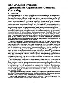
in the event trace for the first and next mention of the edited object. This method aids “what if” experiments, potentially leading to new algorithms. 2. We show the need for abstraction and high-level descriptions of algorithm objects and tags. The details of how objects should be visualized need to be deferred as far as possible in the rendering process. Object tags should be translatable in many different ways, as they can represent different device-dependent colors, or correspondences between multiple views of the same data structures. 3. We show that the kinds of insights provided by algorithm animation are largely influenced by the size of the input dataset. A small, representative input will help the novice understand the intricacies of the pseudocode, while large inputs tend to communicate the properties of the algorithm; they can help indicate the asymptotic behavior. 4. By examining in detail the uses of algorithm animation, we establish the impossibility of instrumenting algorithms to automatically produce useful animations. Although this fact has been mentioned by others [Br88b], the full implications previously have not been examined in depth. 5. We identify several novel features in algorithm animation, and provide implementations to take advantage of them. These include a mechanism for adjusting an algorithm’s pacing to match a recorded narrator’s voice, and a method for moving the camera viewpoint to follow the locus of interest in the animated scene.

Thesis Overview The rest of this thesis examines algorithm animation, its uses, and ways to improve it. Chapter 2 begins with a look back at the wide range of animation systems that have been created since 1980. Chapter 3 takes a step back and compares AA to other emerging technologies. The goal of the chapter is to establish the kinds of uses that AA can be put to, and its inherent need for human guidance. Based on


14

this investigation, Chapter 4 presents features that a good animation system must include, to satisfy the needs of the users just presented. Chapter 5 describes the technical details of an animation system called Gawain which we implemented, seeking to incorporate many of the aforementioned features. This system was used to created web pages and video-tape animations, which are described in Chapter 5. The chapter also describes some interesting technical problems that arose in the implementation, and their solutions. That chapter addresses some limitations of AA when used for debugging. The final chapter summarizes the work, and presents a look at the future, when some of the limitations on AA may be overcome by advances in computer hardware.

Chapter 2 Previous Work Chapter Overview. Algorithm animation has its roots in educational film and in mathematical visualization. It has also been influenced by recent developments in scientific data visualization, which is at present an extremely diverse and active field. Early efforts in algorithm animation in the late 1970’s resulted in an educational film [Ba81] which is still used today. The middle 1980’s saw the development of systems [Br88b][LD85] which allow a user to run algorithms and see animations interactively. Recent efforts have added color and sound [Br91b][Dg92], as well as the use of object-oriented programming [Br91a][AR93][Sc92][EK94]. Section 2.1 provides a survey of systems used to create animations of general algorithms. Excellent overviews of the field [PB93][Ta95] are available, so here we will concentrate on questions that a designer of similar systems must face. Geometric algorithms present special opportunities and difficulties, and systems to make animations for them have also evolved [Sc92][Ge95][TD95]. Section 2.2 gives a survey of these systems. Again, the survey will not be exhaustive but will focus on technique. The past five years have seen the field of algorithm animation flourish. Rather than require the audience to install the animation software on their own computers, researchers have found it convenient to use video tape to record representative sessions. Section 2.3 surveys these video recordings. The videos selected for discussion use interesting animation techniques. 15

CHAPTER 2. PREVIOUS WORK

2.1 2.1.1

16

General systems Sorting out Sorting

The most well-known example of an early algorithm animation is the film “Sorting out Sorting”, created by Ronald Baecker [Ba81] and presented at Siggraph ’81. It explains concepts involved in sorting an array of numbers, illustrating comparisons and swaps. The film ends with a race among nine algorithms, all sorting the same large random array of numbers. It shows the state of the array as a collection of dots in a rectangle; each dot represents a number: x is the array index and y the value. Figure 6 shows a snapshot from the race. In a single screen, nine rectangles with moving dots vividly explain the behavior of nine algorithms. The audience can compare the O(n2 ) and O(n log n) running times of insertion sort and quick-sort. Not surprisingly, quicksort finishes first. The movements of the dots also convey the method used by each algorithm. The film was very successful, and is still used to teach the concepts behind sorting. Its main contribution was to show that algorithm animation, by using images, can have great explanatory power. The film also demonstrated that tools were needed. The effort involved in its production (three years using customwritten software) stimulated research into making more general-purpose algorithm animation systems.

2.1.2

BALSA and Zeus

Many current systems have their roots in BALSA [BS84][Br88b], developed by Brown and Sedgewick in the middle 1980’s. Its influence has been enormous, and by looking at its design one can learn about the problems that any algorithm animation system must solve. BALSA and BALSA-II are general purpose animation systems, which means that in principle they can be used to animate any algorithm. They are primarily used to supplement the teaching of computer programming.


17

Linear insertion

Bubblesort

Straight Selection

Binary Insertion

Shakersort

Tree Selection

Shellsort

Quicksort

Heapsort

Figure 6: A snapshot from the final race in “Sorting Out Sorting”. Quicksort is winning the race.


18

Events: BALSA introduced the paradigm of the interesting event. Not all steps in an algorithm need to be visualized. With some thought, one can identify points in an algorithm where significant changes take place, and mark them. For example, in a sorting algorithm, comparisons and swaps are events. The idea of events reappears in all animation systems after BALSA. In order to animate an algorithm, a programmer using BALSA must implement the algorithm in some programming language, and then modify the resulting program by inserting special procedure calls at the places where interesting events happen. Visualizing events: To continue with the above example, the events must now be visualized. An array of numbers being sorted could be visualized as a row of thin rectangles, each with height proportional to the number it represents. A comparison event might be visualized by highlighting two rectangles, and a swap event by making two rectangles change places. BALSA leaves the task of visualization to the programmer, who must write procedures to visualize events. A collection of these procedures is called a renderer, and produces a view of the algorithm. BALSA takes care of calling these procedures at the appropriate time. Figure 7 shows a screen shot from BALSA. Although in principle any algorithm can be animated, BALSA was intended primarily as an educational tool, and that indeed was its main use. Modifying large programs is a laborious task, and hence it is difficult to use BALSA as a debugging tool in large-scale software development. Moreover, a novel algorithm requires the programmer to write new procedures to visualize events, and this task often proves difficult. On the other hand, because so much is left up to the programmer, the system is very flexible. Clearly, BALSA illustrates a tradeoff between flexibility and ease of programming. Aids to writing renderers: Algorithm animation can be a laborious task, and for that reason BALSA supplies some facilities to make the task easier. When an algorithm uses several renderers, a modeler stores a single representation for the state of algorithm, preventing the duplication of data. Sometimes a new algorithm


19

Figure 7: A screen from BALSA-II, showing the first-fit binpacking algorithm. The two views show the results of using random or sorted data. resembles a previously-animated one, and an adapter can be written to call procedures in the old algorithm’s renderer, thus saving a great deal of programming. Aids to the user: Once an algorithm has been modified, BALSA lets users experiment with it, and watch the resulting animations. Several features make this experimentation easier. BALSA allows the user to simultaneously invoke several algorithms which solve the same problem, in order to learn which one runs fastest. He/she can also run races among several instances of the same algorithm, with each instance taking a different amount of time to perform a given subtask. For example, the user can vary the times taken by comparisons and exchanges, to learn how they affect the running time of a given sorting algorithm. There are cases where a user wants to test an algorithm with a certain type of data, and it may be unreasonable to ask him/her to enter a large amount of input data satisfying some criterion. BALSA provides a solution though input generators. These are menu-driven procedures with a few parameters, which will generate data


20

for a given algorithm. The user can configure an input generator interactively. An example is a generator which produces a nearly-sorted array of numbers, which can be used with several sorting algorithms to see which one best handles this nearlydegenerate case. Zeus After completing his work on BALSA, Marc Brown and others developed Zeus [Br91a], an object-oriented algorithm animation system similar to BALSA. Aware of the difficult task of building renderers, Brown added several features to Zeus that make implementation easier. Zume is a custom pre-processor which generates procedure definitions for renderers from a file of prototype events, and which thus makes it easier to annotate an algorithm with event calls. Another aid to writing renderers is a multi-view editor, which simultaneously displays a graphical image of a view and the textual code which specifies it. The programmer can manipulate either the graphics or the text, and observe the result. This frees the programmer from the need to specify precise positions for graphical elements, for example. The multi-view editor also introduces an interesting feature: the user can change the behavior of the algorithm while it is executing, simply by manipulating one the views. For example, consider a euclidean graph algorithm: the user can move a node in a planar graph to a new location while the algorithm is running, and observe the effect this has on the algorithm’s behavior. Figure 8 is a screen image showing Zeus in action.

2.1.3

“Descendants” of BALSA

AnimA and GeoLab AnimA shares many features with BALSA. AnimA is a system for algorithm animation, and it is written using the facilities of GeoLab, a system for geometric computation. AnimA [AR93] runs within GeoLab [RJ93], and both were developed by P.J. Rezende and others in the early 1990’s. AnimA is a general purpose algorithm animation system, and implements many of the features of BALSA, such as renderers, adapters, and input generators.


21

Figure 8: Zeus: an Animation of Selection Sort. In one control panel, the user has set the relative costs of swaps and comparisons, and in another the input generator determines the initial data. Two views show the algorithm state as plots of sticks and dots. The facilities of GeoLab give users flexibility. To run an animation, a user can choose a problem, an algorithm for that problem, and an input generator for the algorithm. He/she can then run the algorithm, and step through the program events, pause or abort. The use of dynamic libraries allows all the components to be chosen at run-time. Figure 9 is a screen image of AnimA in action. AnimA uses GeoLab’s facilities for program development, which includes a specialized editor that controls access to source code to make it possible for a group of developers to work on large projects consistently. GeoLab GeoLab is an environment for programming geometric algorithms, It is object-oriented and dynamically linked. Within GeoLab, each geometric object has two representations: pure form and graphical form. The purely geometric form of a line segment, for example, is the coordinates of its two endpoints. The graphical form of an object describes how the object should be drawn on the computer screen. Since GeoLab is object-oriented, this description is encapsulated and can consist of


22

Figure 9: A screen image from AnimA, showing the many algorithms implemented on the system programs as well as data. A user can execute a program by choosing data interactively and applying a program to the data. A dispatcher takes care of the task of extracting the pure data from the user’s choice, sending it to the program, then adding the graphic data to the program’s pure output. This feature is used in AnimA. Tango Tango [St90a] was developed by John Stasko in the late 1980’s, and is a general purpose system for algorithm animation. One of the novel features of Tango is its emphasis on smooth animation. Human audiences find it difficult to keep track of events if they occur suddenly and discontinuously, and can understand gradual changes more easily. Tango provides path transitions [St90b], which make it easier for the programmer to specify gradual changes that correspond to program events. The programmer can give the path an object will follow as it moves from one place to another. He/she can also decide how the object’s color will change during the transition, or whether it will fade in or out.


23

Figure 10: A snapshot of Tango on X-Windows, running the first-fit bin packing algorithm. An object of size 5 is being tested for fit into the second bin. Stasko developed an algebra for specifying how to build a transition from several others, by concatenation (which means they happen one after the other), and compositions (which means several transitions happen during the same time period). Recently, Stasko has made his system accessible interactively through the internet [St94], for anyone with a web browser and X-windows. Figure 10 shows a screen image from this version of Tango. Movie and Stills An interesting approach to algorithm animation appears in Movie and Stills [BK91a], programs developed by Bentley and Kernighan. These authors use the Unix text-filter paradigm. In this system, a program is animated by inserting output statements, and not function calls. Each output statement produces a textual description of the changes in the state of the program. This text must be written in a very simple language for describing shapes to be drawn and also identifying program events. In effect, by thus modifying a program, it will itself output a program which, if properly interpreted, results in an animation. One advantage of this approach is language-independence:


24

Figure 11: A race between insertion sort and quick-sort, produced by Stills the original program can be written in any language and run on any machine, since the animation information is communicated through simple ASCII output. Two utilities are provided to interpret a program’s output. The first one, Movie, animates the program on a workstation’s screen. The user can pause the animation, speed it up or slow it down. The other tool, Stills, is a troff filter which allows frames from the animation to be included in printed documents. Figure 11 shows a race between insertion sort and quicksort, produced by Stills. In a way, this system resembles Tango and others which break the algorithm and animation into separate processes. The difference here is that the process communication occurs through pipes or intermediate files, and is in only one direction. This restriction makes it more difficult to animate programs that require graphical input, since the user interface must be written by the programmer. Nevertheless, the system is very easy to learn and use, and can animate many algorithms satisfactorily. Summary: Animating General Algorithms There are several concepts that are relevant to all the animation systems presented in this section. First of all, the idea of an interesting event appears in all the systems. Each time an event occurs, it


25

may lead to a change in an image which the user is viewing. This image visualizes the current state of the program. As the program runs, the state changes, and so does the image. In other words, strictly speaking, what is visualized is not an algorithm but rather its data. From the changes in the image, the user is expected to infer the logic of the algorithm. This leads to another issue, which is that not all events can be visualized with equal ease. It may be easy to write a procedure that swaps two rectangles when two numbers in an array are exchanged, but more effort is needed when representing the act of inserting a key into a red-black tree. Because writing renderers can be difficult, systems like BALSA, Tango and AnimA provide facilities for re-using renderers from related algorithms.

2.2

Geometry-oriented Systems

Designers of geometric algorithms face special challenges. While much of their discipline uses visual objects, computers deal with numbers and symbols. As a result, geometric objects in a computer program must be represented in a form which is difficult to translate back into images. Hence computational geometry can benefit from visualization. Another reason for visualizing geomtric algorithms is its relative ease. As we saw in the previous section, the most laborious task in writing an animation is writing renderers that portray the program data as images. In the case of geometric algorithms, the program data contains positional information, and hence can be drawn on the computer screen without the need for translation. For these reasons, since about 1990 several systems have evolved that try to satisfy the needs of computational geometers. This section examines them.

2.2.1

Two-dimensional Systems

Workbench By 1990, Epstein, Sack, and others had developed their Workbench for Computational Geometry, which is an environment for developing, implementing,


26

and testing geometric algorithms. One of their goals was to measure the actual cost behavior of published algorithms. They were concerned that many published geometric algorithms had not been implemented, and that the costs of these algorithms were given only in asymptotic form. The authors wrote a library of abstract data types and of elementary (constantcost) geometric operations. Using this library, they implemented several published geometric algorithms, which addressed the following two-dimensional problems: convex hull, polygon triangulation, visibility, point location and line segment intersection. Geometric algorithms often use complex data structures, whose performance impacts the algorithm’s. Hence the authors implemented several search trees (binary, splay, AVL, and finger trees), and tested them independently. They also develop a method for generating random simple polygons. The workbench includes a facility for animation. Each algorithm has a corresponding animation module, which visualizes the events. Animation can affect timing measurements, because events are visualized as they happen, and the rendering time must be omitted from time cost calculations. Since timing is a major goal of the workbench, the authors use a flag to disable rendering as needed, incurring a small constant overhead. In this fashion the same code can be measured or animated. Figure 12 shows a screen dump from the workbench. XYZ Geobench Peter Schorn’s XYZ Geobench [Sc92], created around 1990, provides tools for writing and testing geometric algorithms. It provides a library of geometric abstract data types. The Geobench emphasizes robust computation. For example, a poorly-implemented algorithm for segment intersections may not detect points where more than two segments coincide. To this end, the Geobench provides tools for creating degenerate data which is useful for torture-testing algorithms. Geobench is limited to two-dimensional problems, although it has some simple animation facilities. Basically, a programmer wishing to animate an algorithm must visualize the program events directly. This means that for each event, the programmer must write code which draws the geometric changes, pauses to let the user see them,


27

Figure 12: A snapshot from the Workbench for Compuational Geometry, showing a visibility algorithm on a triangulated polygon. then continues. Nevertheless, interesting animations are possible. Figure 13 shows a sweep-line algorithm for the Voronoi diagram in action.

2.2.2

Beyond Two Dimensions

For both the Workbench and the Geobench, the emphasis is on the implementation of geometric algorithms, not on glossy renderings. Moreover, their algorithms are restricted to two-dimensional geometry. Two systems choose a different approach, concentrating on the presentation of geometry in three and higher dimensions. Geomview Geomview [Ge95] is a group effort from the Geometry Center of the University of Minnesota. The program is essentially a sophisticated viewer for geometric data. Users can interactively control the appearance of objects, by changing the lighting, shading and material properties of the surface. Phong shading leads to realistic-looking objects. Moreover, three- and four-dimensional objects can be viewed with perspective, orthogonal, hyperbolic and spherical projections. The appearance and display of geometric data can also be controlled through


28

Figure 13: A snapshot from Geobench, showing a sweepline algorithm for the Voronoi diagram of points on the plane. software. Geomview includes an interpreter for a lisp-like command language, through which a program can control all of the system’s features. Objects displayed by Geomview can consist of polyhedra, quadrilaterals, meshes, vectors and Bezier patches. The description of an object can either be stored in files, or can be generated by a separate program which sends its output to Geomview through a pipe. Figure 14 shows Geomview in action. This latter feature makes it possible to animate geometric algorithms with Geomview. A programmer needs to modify a program to output descriptions of geometric objects in a Geomview format, and in this way use Geomview as means to visualize the program’s behavior. This approach is thus the only way to animate an algorithm, since Geomview has no built-in methods for animation. An enthusiastic programmer can also use Geomview for interaction with a user, since Geomview can be configured to inform a program if a user selects a geometric object with the mouse. Geomview’s versatility is shown in the wonderful movies [EG91] [LM94] [LM95]


29

Figure 14: Geomview in action, showing the approximate convex hull of points in convex position. that have been made with its help. Of course, with all that versatility comes complexity: not only is Geomview a very large piece of software, but also users may take some time to learn its special features. GASP GASP [TD95] aims to provide high-quality animations of geometric algorithms with minimal programmer effort. It tries to achieve the high-quality renderings of three-dimensional objects that Geomview provides, while minimizing the effort needed to create them. The spirit of GASP is to separate geometry from animation. To animate a geometric algorithm, a programmer inserts some function calls which tell GASP which geometric objects have been added or removed. This is usually easy to do, since the coordinates of the geometric objects are already known to the program. Based on the information passed through function calls, telling it of the changes in the scene, GASP then decides how to represent these changes. Changes in a GASP animation are grouped into atomic units. These correspond to transitions in TANGO. Within each atomic unit, there can be several changes to the data. For example, several facets of a polyhedron may be simultaneously removed during one atomic unit. In the spirit of TANGO, the changes are usually smooth. The changes to a scene can be represented in several ways. A new object can


30

fade into place, blink as it appears, or move in from outside the scene. Conversely, removed objects fade out gradually, or move away. There are defaults for all the aspects of how the change is represented, including the type of change, the time it takes, the colors used, etc. These defaults are stored in simple text style files that the programmer can modify as necessary. This use of defaults means that novice programmers can produce simple animations without learning all the details of the system. The system includes a user interface that follows the model of a video tape recorder. The user can view the animation forwards or backwards, at normal or high speed. Advantages of GASP include its ability to represent 3D geometry, high production values and good color facilities. In particular, the range of colors that are attractive and easy to see on a computer monitor is not the same as the colors that are suitable for recording on video tapes. Bearing this difference in mind, the style files in GASP can be set to use colors most suitable for the output medium being used. Another good aspect of GASP is that it frees the programmer from learning about computer graphics or rendering of three-dimensional geometry. Programmers are free to concentrate on geometry. Figure 15 shows a scene from a GASP-generated animation, which was composed in just a few hours. Of course, GASP does have some limitations. The most obvious one is that it is mainly limited to geometry. This means that, if used to animate general algorithms, the programmer must be familiar with geometry. Another drawback lies in the rewind facility which is slow, although this difficulty arises from the implementation and not from a weakness in the design. It should be simple to remedy.

2.2.3

Mocha

The web is an excellent medium for textual explanation. Java is a good portable language. If we use both, we can mix animations with explanations. This is the goal of Baker et al’s Mocha [Ba96] system. Running algorithm animations on web pages leads to several difficulties. It exposes


31

Figure 15: A snapshot from GASP, showing an object that cannot be taken apart with two hands using only translations. the algorithm’s code to the public, which may be undesirable. It also forces the user to download and run a potentially large program, which can take time. More significantly, it requires the programmer to re-implement existing algorithms in Java, in order to make them run on the user’s browser. The programming effort involved can be significant. Mocha’s authors address these problems by splitting the animation into two: the user downloads a graphical interface and animation engine, which are small units of code whose function is to interpret events sent by the algorithm. The algorithm, however, remains on the server. The algorithms can retain their original implementations, with minor modifications where interesting events occur. This approach resembles Bentley and Kernighan’s Anim [BK91a] above, which also separates algorithm and animation into two independent processes.


2.3

32

Visualizations

In any field, skill in the use of tools is acquired not only by studying the tools themselves, but also by studying the products of other skilled workers. Whereas in the previous sections we considered the tools, ie systems which can be used to create animations of algorithms, in this section we focus on the products of these tools, the actual animations. This section will focus mainly on videos published in the Annual Video Review of Computational Geometry, which is the main vehicle for dissemination of techniques in the field. The field of algorithm animation is rich, and still growing. As they seek to explain algorithms, researchers borrow techniques from related disciplines such as scientific and mathematical visualization, and interactive environments. As a result, we find in these videos examples not only of algorithm animation [VR1a,c,d,f,g,i,j, 2b,c,d,e,h, 3a,b,c,g, 4b,d], but also mathematical visualizations [VR3e,4e,4f] and interactive visualizations [VR1e,2a,3f,h,4a,c]. In addition to the Video Review, we will also briefly discuss three films from the Geometry Center [EG91] [LM94] [LM95]. This section does not aim at a thorough review of all the videos extant, but rather seeks to present specific animation techniques which are used in some of them. These techniques (i.e. tricks used twice!) turn a video into more than simply “dancing data”. Animations may depict how an algorithm processes its data, but they should also explain the reasons for particular actions.

2.3.1

Mathematical Visualization

Before considering animations of geometric algorithms, it may help to consider three movies produced at the Geometry Center of the University of Minnesota. They were all produced with Geomview, as well as other software. Not Knot [EG91] introduces the viewer to knot theory, by considering the complement of a knot. Visualizing the complement of the Borromean rings leads to a brief excursion into hyperbolic geometry. Outside In [LM94] visualizes the remarkable theorem which states that a sphere in three-space can be smoothly everted, in other words, turned inside out. The Shape of Space [LM95] visualizes toroidal space.


33

Figure 16: A sphere is smoothly turned inside-out, from the film “Outside In”. It explains, in more detail, some concepts that were brought up in Not Knot. All three films show that a great deal of effort went into their production. They achieve the difficult task of explaining problems in topology to novices. The production costs of these films are relatively large. For example, Outside In took 2-3 person-years of programming effort, in addition to the time needed to develop generalpurpose tools for geometric visualization. Once the tools were developed, production was easier. The last film, The Shape of Space was produced in only four months. Even with proper tools, the need to make the film accessible to novices required additional effort. If a concept taxes the audience’s geometric imagination, then its explanation will tax the film-maker’s imagination as well. Figure 16 shows a montage from Outside In. A short video, Animating Proofs [VR4f] uses a couple of techniques to effectively illustrate Pythagoras’ Theorem. The narrator reads the proof of the theorem from Euclid’s Elements, and whenever a geometric object such as a line or point is mentioned, the corresponding graphical element is highlighted. Through this simple trick of timing, the burden of referring back and forth between proof and diagram is avoided. Another simple trick is used when two triangles are shown to have equal areas. One


34

triangle is smoothly deformed into the other.

2.3.2

Demonstrations

Several of the video segments [VR1b,1h,2f,3d] contain animations of algorithms, but are primarily intended to demonstrate the capabilities of an algorithm animation system. To enable the viewer to concentrate on the capabilities of the system, these demonstrations tend to animate well-known algorithms, e.g. Graham’s scan. For this reason, they will not be considered here.

2.3.3

Algorithm Animations

Optimal Two-Dimensional Triangulations [VR1c] shows a typical use of color. The video animates versions of an algorithm that computes optimal 2-d triangulations. Each triangle is colored according to some measure, such as maximum vertex angle. Optimal triangulations minimize that measure. As the algorithm runs and the triangulation is improved, its overall color approaches the optimal one (see Figure 17). Boolean Formulae for Simple Polygons [VR1d] uses color and also multiple views to convey information. The algorithm computes the boolean formula for a polygon: given the half-planes determined by each edge of the polygon, the boolean formula is the combination of OR’s and AND’s of these halfplanes that defines its interior. For a convex polygon, AND’s suffice, but concave polygons require OR’s as well. The animation uses multiple views, which simultaneously show the state of the algorithm in different ways. One view shows a tree of partially-satisfied polygons, and another shows the same tree in schematic form (see Figure 18). Through the schematic tree, the user sees at glance how certain types of polygons lead to very unbalanced trees. Another view shows, in text form, the boolean formula as it is built, and finally there is a view that shows the edges of polygon being processed by algorithm. Each view corresponds to a way of abstracting the information being processed by the algorithm. Like the previous animation, The New Jersey Line-Segment-Saw Massacre [VR1j]


35

Figure 17: A still from “Optimal Two-Dimensional Triangulations”. The polygonal outline of the USA is being triangulated. Lighter triangles have larger minimum angles.

Figure 18: A still from “Boolean Formulae for Simple Polygons”


36

Figure 19: A still from “The New Jersey Line-Segment-Saw Massacre” uses multiple views to explain an algorithm. This time it is Chazelle and Edelsbrunner’s optimal sweepline algorithm for general line-segment intersections. As the sweepline advances, a separate view shows the red-black tree holding partiallyprocessed segments. The video is difficult to understand, mostly because the algorithm itself is very complicated. Perhaps many more views would have shown in detail what was going on, but the authors may have feared overloading the viewer’s ability to keep track of too many simultaneous changes. The time limitations of the video also preclude the necessary drawn-out explanation. Figure 19 shows a still from the video. Building and Using Polyhedral Hierarchies [VR2b] shows that often multiple views are not needed. It shows a polyhedron being simplified as certain vertices and their incident edges are removed (see Figure 20). Implicitly, a hierarchy of simpler polygons is built, although the viewer does not need a visualization of it to understand it. The video also shows the use of color to encode time information: each changed polygon facet is drawn in a new color, and this trick allows the viewer to see the algorithm’s history at a glance. In theory, the systems described above can be used to visualize a new idea, with the


37

Figure 20: A still from “Building and Using Polyhedral Hierarchies” visualization appearing simultaneously with the research paper that presents the new concept. In practice, however, most algorithm animations describe ideas which are already well-known. Objects that Cannot be Taken Apart With Two Hands [VR2h] (see Figure 15) is remarkable for appearing at the same time as the discovery it explains. An Animation of a Fixed-Radius All-Nearest Neighbors Algorithm [VR3c] is an excellent video. The algorithm described here solves the following problem: given a set of points and a distance δ, find groups of points where each member of the group is within δ of the others. The algorithm uses a scan line to partition points into an adaptive grid, made up of horizontal and vertical slabs of width ≥ δ. Occupied grid entries are identified by labelling each point with its grid coordinates, and then sorting the list of labels. Points with the same label lie in the same non-empty grid square. Finally, these grid entries are scanned for pairs of points within δ of each other, and these pairs are reported. The animation is skillfully made. The narration is well-synchronized with the video. For example, labels appear just after they are mentioned. Skill is also evident in the use of multiple views. One view shows the search tree which stores point labels.


38

Figure 21: A still from “An Animation of a Fixed-Radius All-Nearest Neighbors Algorithm” The sorted list of labels corresponds to the bottom level of the tree. The animation first shows this list, then fades in the search tree on top of it (Figure 21). This approach is preferable to showing the insertion of each label, which leads to much confusing extraneous activity. The video closes with a three-dimensional application of the algorithm: finding an isosurface of a molecule. This section is harder to follow, perhaps because elements are not labelled, forcing the viewer to remember the identity of each element.

2.3.4

Interactive Visualizations

This section examines a class of systems which are better classified as interactive visualizations than as algorithm animations. The videos selected here demonstrate interactive systems which illustrate an algorithm through its results. By contrast, most algorithm animations show the viewer an algorithm’s behavior. With an interactive visualization, the user can change some graphical data interactively, and immediately see the resulting structure produced by the (usually geometric) algorithm under consideration.


39

Figure 22: A still from “Visualizing Fortune’s Sweepline Algorithm for Planar Voronoi Diagrams”. We can see the sweepline, the parabolic fronts, and the partially constructed Voronoi Diagram. Visualizing Fortune’s Sweepline Algorithm for Planar Voronoi Diagrams [VR2a] does indeed animate that algorithm for building a Voronoi diagram, but its main goal is to demonstrate an interactive tool for exploring the properties of Voronoi diagrams. Given a set of points in the plane, the user can turn several structures on and off. These structures are the points themselves, their Voronoi diagram, Delaunay triangulation, or convex hull. The user can also add an abitrary paraboloid of revolution, project points onto it, add tangent planes, and verify that the paraboloid’s lower hull indeed corresponds to the Voronoi diagram. Since this is a video tape, the viewer can’t control the system, but must watch a recording of the author’s interaction with the system. Nevertheless, the video shows the advantage of giving the user the ability to turn aspects of a visualization on and off. Figure 22 shows Fortune’s algorithm in action. Exact Collision Detection for Interactive Environments [VR3f] presents a realtime system that detects collisions between polyhedral objects. If two features like a vertex and an edge are close together, the system displays a line between them,


40

Figure 23: A still from “Exact Collision Detection for Interactive Environments”. Look carefully, and you will see that only objects whose bounding boxes overlap (the cube and the fingers) trigger distance calculations (the lines from the fingers to the cube face). indicating that those two features are being tested for collision. To the user, this produces the illusion of elastic filaments joining adjacent features on neighbouring objects. The video then demonstrates the use of bounding volumes. Two objects are tested for collision only if their bounding volumes intersect. The effectiveness of this acceleration technique is immediately apparent, since the filaments appear only when bounding volumes meet, and their number is greatly reduced (Figure 23). We can see the effect of an algorithmic technique even though we are only shown the product of the algorithm.

Chapter 3 Theoretical Considerations Introduction Is algorithm animation art or science? This chapter addresses that question. It is a useful question to ask, because it touches on the nature of technology and the best way to use it. We will show that a good AA system is neither manual nor automatic, but rather an interactive tool. We will also show that algorithm animation is characteristic of a new, maturing field, studying ways to use computer technology. Let us define our terms. Defining “art” and “science” is too difficult, and takes us too far afield, so we will restrict ourselves to visual arts and computer science, respectively. More specifically, we will consider the techniques that AA borrows from both disciplines, and compare their goals. Borrowed Techniques Algorithm animation borrows techniques from both visual arts and computer science. Visual artists use color, movement and composition to express emotions and ideas, and so does AA. Animations explain computer algorithms, and are implemented on computers, so they use computer science techniques by definition. These techniques are many, but they include parsing, message passing, graphics, software engineering, and object-oriented programming, as our review of literature (Chapter 2) has shown.

41

CHAPTER 3. THEORETICAL CONSIDERATIONS

42

Similar Goals We shall compare the goals of AA to those of visual art and scientific visualization. As we shall argue below (§3.3.1), computer scientists need to visualize algorithms that are difficult to understand from source code alone. Thus AA aims to express what cannot be said simply, to convey subtle ideas that are difficult to verbalize. In this respect, its aims resemble those of visual arts. Scientific visualization also shares similar goals, since it also seeks to explain information visually. Tufte’s works [Tu83, Tu90, Tu97] are good evaluations of techniques for visualizing scientific data. Our goals are analogous to his. In a broad sense, computer science is the study of automatic processes (ie, algorithms) and techniques. Algorithm animation is used to explain these techniques to others, but it can also be used to further their study. As we explain below (§3.2), it can be used to help discover new algorithms. Thus it shares a common goal with other branches of computer science: exploration and discovery. Avoiding Automation Many subfields of computer science aim to automate tasks traditionally done by humans. In some cases, they aim to build synthetic equivalents of human activity. Examples include artificial intelligence, which aims to build synthetic consciousness, robotics, whose goal in some sense is building synthetic human bodies, and formal methods, which aim to take over the difficult human task of ensuring software reliability. Computer graphics in a sense aims to replace the human photographer or artist. These descriptions are of course over-simplifications, perhaps caricatures of branches of computer science. But I’ve stated them in this way to emphasize that the ultimate goals are very ambitious. As we shall see below (§3.1.2.1), in several cases those ambitious goals have been modified over time to recognize the need for human participation. An idea central to this chapter is that, although AA can be used to develop methods for automation, it cannot itself be automated. In other words, algorithm designers cannot see their creations effortlessly animated. We will never achieve the


43

dream of expressing an algorithm as an implementation, and then feeding the code into a general-purpose animation machine, expecting a beautiful animation as a result, perfectly timed and narrated. We shall try to establish this point at several places in this chapter. By arguing this way, we seek not only to establish the point, but also to explore the subject at hand. Our aim is twofold: to dissuade others from developing automatic animations, and to establish the attributes of an ideal animation system. Our argument will have two stages. The first (§3.1) will consider the historical development of computer science, and compare it to two other technologies: perspective drawing and motion pictures. Technology changes with time: initially it inspires fascination, and is pursued for its own sake, but at a later stage it becomes widely accepted and becomes more practical and useful. There is evidence that computer science is going through this process of maturation. Algorithm animation is characteristic of this later stage. This mature stage can be seen most clearly in the change in attitude towards Artificial Intelligence over the years. Whereas the initial dream of AI was that computers would someday do tasks that humans do well, opinion has since shifted. Now, we recognize that computers excel at some tasks, and humans at others. Effectively, computers can help humans communicate and think better, but they cannot replace them. The second stage of the argument (§3.3.4) will consider a limited version of automatic AA, and will show that this too is an unrealistic goal. Algorithm animations are aimed at a human audience, and the needs of this audience cannot be met by a purely automatic process. To be useful, animations must be crafted with care, and this care requires intensive participation by a human animator. Thus an ideal animation system needs to ease such participation, and must be highly interactive. The final stage of the argument addresses the needs of a human audience, so we need to learn who this audience is (§3.2), how they use AA, and what they need from it. The sections preceding the second argument will examine the need for visualization (§3.3.1), the need for interactivity (§3.3.2), and the need for a large library of visualization techniques (§3.3.3). The chapter concludes by summarizing the argument in the form of propositions. We list them here to guide the reader:


44

Proposition 1 Algorithms benefit from visualization (§3.3.1). Proposition 2 Algorithm visualization needs interactivity (§3.3.2). Proposition 3 Algorithm animators need a large library of visualizations (§3.3.3). Proposition 4 Automatic algorithm animations can be unsatisfying (§3.3.4).

3.1

Technological Maturation

As a rule, algorithm animations are not flashy. They tend to avoid eye-catching displays that stimulate the senses, as TV commercials do. Why is this so? As we shall see, there are straightforward reasons, having to do with the purpose of AA and with the environment in which it grew up. But there is another, historical reason for AA’s self-restraint.

3.1.1

Explanation vs. Entertainment

The first prosaic reason is that the purpose of AA is explanation, and dazzling is opposed to this goal. A novice student learning an algorithm may be stunned by colorful, dynamic graphics, but will likely not learn from them, no matter how strong their impact, perhaps because their impact is distracting. Similarly, a researcher developing a new algorithm will want a simple, expressive animation system. Spinning text and flashing colors draw the viewer’s attention away from the subject at hand, and obscure the purpose of AA, which, after all, is explanation. Secondly, AA has developed within an academic environment, with goals different from the commercial entertainment world. From its inception in SOS [Ba81] and BALSA [Br88a], AA has been developed by computer scientists, especially geometers, and they have preferred direct expressiveness to glossyness. This trend towards austerity has notable exceptions. Among them are Jim Blinn’s educational videos [Bl94] [Bl85], which use clever ways to engage and amuse the viewer, while conveying ideas in mathematics and physics. The techniques used are nevertheless not gratuitously flashy.


a

45

b

Figure 24: Evidence of maturating use of perspective: a) Perugino, “The Delivery of the Keys”: perspective as conspicuous spectacle. b) Pieter de Hooch, “The Bedroom”: perspective as inconspicuous tool. Finally, AA is tied to technological development, and is typical of its later stages. As we will see in the next section when computer technology matures, novelty alone no longer moves the popular imagination. When this happens, the technology can be used more effectively. Algorithm animation manifests this change.

3.1.2

Historical Parallels

We can see this maturation from novelty into every-day use in two other technologies: mathematical perspective and movies. Like AA, they are marriages of artistic and mathematical techniques. As an art historian explains, As Italian artists became more comfortable with mathematical perspective in the course of the fifteenth century, they came to rely less on peepholes and formulas, and be less fascinated by the linear forms (such as tiled floors and buildings) that had been the hallmark of early Renaissance style [St95]. We can see this artistic change of attitude in Fig. 24. Perugino (Fig. 24a) is fascinated by perspective, which dominates his painting, while the de Hooch (Fig. 24b) uses it as a tool 100 years later.


a

46

b

Figure 25: Popular conception of computers, then and now: a) A machine room with whirling tape drives. b) A web browser. Similarly, early cinema was full of spectacular displays, whose sheer novelty fascinated the viewer: Early audiences went to exhibitions to see machines demonstrated (the newest technological wonder, following in the wake of such widely exhibited machines and marvels as X-rays or, earlier, the phonograph), rather than to view films. It was the Cinématographe, the Biograph or the Vitascope that were advertised on the variety bills in which they premièred, not Le Déjeuner de bébé or The Black Diamond Express [Gu90]. Early film showings included lengthy descriptions of the projection machinery, which interested the audience as much as or more than the images it cast. But in time, both these technologies matured, and came to be taken for granted. 3.1.2.1

Computers Then and Now

The perception of computers in the popular mind is also changing from novel to commonplace. We can observe this change in perception in two aspects of computers: the way they look and their perceived intellectual capacity. This latter aspect relates to automatic AA.


47

The high cost and scarcity of the first computers made them spectacular. Many films presented computers the way the public imagined them: an air-conditioned machine room with whirling tape drives (Fig. 25a). After personal computers arrived, ordinary people saw that the machines could also be used for communication. Today, the average person’s image of a computer is a web browser, showing linked and active images (Fig. 25b). Beyond their physical appearance, early fascination with computers involved the optimistic hope that many higher human functions could be automated. The public and researchers expected to find a relatively simple mechanism that would allow computers to reproduce human intelligence. But everyday experience overwhelms simple automatons, whereas humans can handle it well. We humans aren’t sure what this experience is, so we can’t tell computers how to process it. The past decade has seen a change of attitude. Only certain tasks can be automated, and only human beings can provide the guidance and common sense that machines lack. Expert systems, a successful product of AI, try to use human expertise and incorporate it into a decision database. In a sense, expert systems acknowledge that human beings are more knowledgeable than computers can hope to be in the near future. Recently, photorealistic computer graphics has also undergone a change of attitude. Ray-tracing and radiosity methods originally promised to accurately mimic the photographic camera. They have achieved large strides, but in a sense have been too successful. Photorealistic images tend to portray idealized scenes, without the subtle lighting and surface details that we are used to seeing in the real-world. That may account for the increased research into non-photorealistic rendering in recent years. Non-photorealistic rendering tries to incorporate well-known artistic techniques to make expressive illustrations. In other words, it tries to blend visual arts with computer science. Both AI and computer graphics have had to take into account the complexity of human thought and perception, and have tried to incorporate established human expertise into their methods, through the use of expert systems, for example. This development in another branch of computer science is relevant to our argument, because AA is a set of techniques for visually communicating the behavior of algorithms to


48

humans. Just as reasoning cannot easily be animated, explanation also defies automation. It cannot be automated because there is no easy way to encapsulate within a computer system the needs and habits of the human audience. Algorithm animations are produced by humans with the assistance of a computer tool. Just as education requires human teachers, algorithms need human animators. This provides partial proof for Prop. 4. 3.1.2.2

Summary

As technology matures, it becomes more practical and less spectacular, less an object of fascination. Computer science’s maturity is reflected in attempts to incorporate human talents, instead of trying to replace them with automatic mechanisms. Algorithm animation reflects this change in attitude. Forward View We have seen that AA typifies the maturation of computer science, as the potential and limitations of computers become clearer. The rest of this chapter looks at how AA is used, and what its users need from it. We need to establish these basic facts to better explain why automatic AA is an unreasonable goal. The next two sections take up the uses of animation (§3.2) and the needs of its users (§3.3).

3.2

Uses of Algorithm Animation

Algorithm animations can be aesthetically pleasing, even entertaining, but they remain attached to their main goal, which is explanation. In this section we will examine the ways in which animations are used to explain algorithms. Who needs algorithm explanations? People inventing the algorithms for the first time (designers), people who are implementing them and run into bugs (implementers), and those who are learning about an algorithm for the first time, be they experts or novices (communication). This section will merely identify the kinds of people who use AA, and give rough


49

sketches of how they use it. Having established the users’ roles, the subsequent section identifies their needs.

3.2.1

Algorithm Design: Rapid Prototyping

A scientist developing a new algorithm may use animation as a tool. Although the process of inventing algorithms is not well understood, we can identify some of the steps involved. For instance, an algorithm designer may write several possible pieces of code while searching for the one s/he needs. Much of the code will not suit the designer’s ideas, and will be discarded. The designer needs a system for rapid prototyping, that makes it easy to compile and run small programs. Animation can help this stage by giving the designer a clearer view of the algorithm’s behavior, but should require minimal effort from the designer. Otherwise, the scientist’s mental energy will be spent on programming details, and not on design. Algorithm designers also need to experiment with their algorithms’ behavior, by manipulating the data. They will want to try different inputs, or inputs with different characteristics. For example, Fortune’s sweepline algorithm for the voronoi diagram assumes non-degenerate inputs, ie, no four sites are co-circular. On degenerate inputs, the algorithm yields wrong results, as in Figure 26, where eight sites are co-circular. Designers will also want to vary the behavior of the algorithm by manipulating the data in mid-execution. While watching an AA, they might want to alter an internal data structure. If the change has favorable results, it might lead the designer to adopt it as a permanent change in the algorithm. In this way, algorithm design proceeds partly by insight and mostly by experimentation.

3.2.2

Implementation: Debugging

Once an algorithm has been developed, it must be implemented and debugged. Debugging is difficult, and at present we lack a formal description of what is difficult about it. One reason for the difficulty has been suggested: bugs are hard to find because the programmer does not have a clear understanding of the program’s state


50

Figure 26: Fortune’s sweep: The implementation fails on degenerate inputs [Ei97]. Making a picture of the state can often be useful. Consider Fig. 27, which shows a bubble-sort when the input consists of numbers sorted in reverse order. Throughout the animation, the leftmost stick (representing the first number in the array) remains stationary. This suggests an off-by-one bug, and closer scrutiny reveals that j=1 should read j=0. Thus sometimes animation helps to find bugs by inspection. The exploratory nature of debugging can also make it amenable to animation. Debugging often involves inspecting and modifying program data in mid-execution. If a programmer uses an animation system that lets him/her interactively change program data as the program is running, s/he will be able to see the results of this experimentation graphically, and may isolate the bug.

3.2.3

Communication

As we have just seen, algorithm designers and implementers can use AA. In these contexts, animation serves to explain an algorithm to its author, because it illuminates aspects of the algorithm that the author was unaware of. However, algorithm


51

for (i=0; i pivot); while (a[++j] < pivot); if (i

web-based animation of geometric algorithms

web-based animation of geometric algorithms

Suggest Documents

Geometric Algorithms

Geometric Algorithms

Geometric Algorithms

Geometric Approximation Algorithms - CiteSeerX

Geometric Approximation Algorithms - CiteSeerX

OE ciency of Geometric Algorithms

Computational Geometry Algorithms for Animation

Geometric, Variational Integrators for Computer Animation

Geometric Approximation Algorithms - Semantic Scholar

Geometric Tools for Algorithms - CiteSeerX

Empirical Design of Geometric Algorithms - Semantic Scholar

Geometric algorithms for manufacturing of freeform

Empirical Design of Geometric Algorithms - CiteSeerX

Webbased Educational Resources - MUHS

Physically Based Animation and Rendering of Lightning - Geometric ...

NSF CAREER Proposal: Approximation Algorithms for Geometric ...

Randomized Algorithms for Geometric Optimization Problems*

Competent Algorithms for Geometric Semantic Genetic Programming

Robust Geometric Algorithms for Sensor Planning ... - CiteSeerX

Animating Geometric Algorithms Over the Web - CiteSeerX

CONSTANT-WORK-SPACE ALGORITHMS FOR GEOMETRIC

Two Geometric Algorithms for Layout Analysis - CiteSeerX

Animating Geometric Algorithms Over the Web - CiteSeerX

Simplification Envelopes - Geometric Algorithms for Modeling ...