for each Web page based on HTML tags (and not content) in the page, and the ... tag sequence of the page. Observe that S ..... as well, with the type set to âfollowing-sibling-tag-iâ etc. for ... We add the following features for the left anchor text.
Web-Scale Information Extraction with Vertex Pankaj Gulhane #1 , Amit Madaan #2 , Rupesh Mehta ∗3 , Jeyashankher Ramamirtham #4 , Rajeev Rastogi #5 , Sandeep Satpal ∗6 , Srinivasan H Sengamedu #7 , Ashwin Tengli +8 , Charu Tiwari #9 #
Yahoo! Labs, Bangalore, India, ∗ Microsoft IDC, Hyderabad, India, {1 pankajeg,
+
Microsoft IDC, Bangalore, India
2
amitm, 4 jeyashan, 5 rrastogi, 7 shs, 9 charu}@yahoo-inc.com 3 { rupeshme, 6 ssatpal, 8 ashwint}@microsoft.com
Abstract— Vertex is a Wrapper Induction system developed at Yahoo! for extracting structured records from template-based Web pages. To operate at Web scale, Vertex employs a host of novel algorithms for (1) Grouping similar structured pages in a Web site, (2) Picking the appropriate sample pages for wrapper inference, (3) Learning XPath-based extraction rules that are robust to variations in site structure, (4) Detecting site changes by monitoring sample pages, and (5) Optimizing editorial costs by reusing rules, etc. The system is deployed in production and currently extracts more than 250 million records from more than 200 Web sites. To the best of our knowledge, Vertex is the first system to do high-precision information extraction at Web scale.
I. I NTRODUCTION Vertex is a system developed at Yahoo! for extracting structured records at Web scale from template-based Web pages. As an example, consider the page shown in Figure 1 for restaurant “Chimichurri Grill” from the aggregator Web site www.yelp.com. The page contains a wealth of information including details like the restaurant name, category, address, phone number, hours of operation, user reviews, etc. Vertex can extract this information from such detail pages, and store the extracted data for each page as attributes of a record as shown below. Name Chimichurri Grill 21 Club
Category Argentine Steakhouses American
Address 606 9th Ave NY 10036 21 West 52nd St NY 10019
Phone (212) 586-8655 (212) 582-7200
··· ··· ···
A. Applications Extracting records from Web pages has a number of applications which include improving Web search results quality, Web information integration, etc. For example, if a user were to type a restaurant search query, then rank ordering the restaurant pages in the search result in increasing order of distance from the user’s location will greatly enhance the user experience. Enabling this requires us to extract addresses from restaurant pages. Furthermore, integrating information extracted from different product Web sites can enable applications like comparison shopping where users are presented with a single list of products ordered by price. The integrated database of records can also be accessed via database-like queries to obtain the integrated list of product features and the collated set of product reviews from the various Web sites. ∗,+ Work
done while authors were at Yahoo!
Fig. 1.
Example restaurant detail page.
B. Wrapper Induction Vertex uses Wrapper Induction [9], [13], [10] to extract data from head sites like www.amazon.com and www.yelp.com that contain thousands or even millions of script-generated pages adhering to a common template. Human editors annotate the attribute values to be extracted on a few sample pages belonging to each Web site, and the annotations are then used to learn extraction rules for each site. Since pages of a Web site have similar structure, rules that are learnt from sample pages can be used to extract attribute values from remaining pages of the site. A key benefit of wrappers is that they ensure high precision without incurring inordinate amounts of human effort. This is because the cost of annotating a few pages per site is amortized over thousands or even millions of pages belonging to the site. C. Our Contributions While the idea of using wrappers for extraction is not new, Vertex differs from previously built prototypes and systems in two key aspects: •
•
Vertex brings together diverse technology components incorporating novel algorithms to handle the complete extraction lifecycle, from clustering pages within a Web site, to learning extraction rules, to detecting site structure changes, and finally relearning broken rules. Vertex has been deployed in a production environment within Yahoo! to extract data from more than 250 million crawled Web pages belonging to ≈ 200 Web sites. To the
best of our knowledge, Vertex is the first system to do high-precision information extraction at this scale. In this paper, we describe the architecture and implementation details of the Vertex system. To operate at Web scale, Vertex relies on a host of algorithmic innovations: 1) Clustering algorithm for grouping similar structured pages in a Web site. Our algorithm makes only 3 passes over the data. 2) Greedy algorithm for picking structurally diverse sample pages for annotation. 3) Apriori [1] style algorithm for learning very general XPath-based extraction rules that are robust to variations in site structure. 4) Site change detection scheme that monitors a few sample pages per site, and subjects the pages to different structural and content tests. 5) Algorithm for optimizing editorial costs by reusing rules. In addition to implementation details, we also present experimental results on real-world crawl data from Web sites. Our experiments (a) demonstrate the effectiveness of our rule learning algorithms – our extraction rules had an average precision of close to 100% and recall above 99% across a broad range of attributes, (b) enable us to determine system parameter settings like sample sizes for clustering, and (c) provide insights into Web phenomena like frequency and characteristics of site changes. II. OVERVIEW As mentioned earlier, Vertex learns extraction rules from human annotated sample pages, and then uses the learnt rules to extract records from pages of Web sites. Vertex extraction rules are in XSLT format, and contain highly generalized XPath expressions that are robust to variations in site structure ensuring high precision for extracted attribute values. The input to Vertex is the list of Web sites from which records are to be extracted. Web sites can belong to different verticals like product (e.g., www.amazon.com), business (e.g., www.yelp.com), news (e.g., www.cnn.com), video (e.g., www.youtube.com), etc. We define a separate schema for each vertical. The schema for the product vertical contains attributes like product name, brand, description, image, price, etc. while the schema for business contains attributes like business name, category, address, phone number, rating, etc. Attributes can satisfy one or both of the following two properties: constant or mandatory. The value of constant attributes does not change over time – e.g., product name is a constant attribute while price is not a constant attribute. Mandatory attributes are the ones that are present on every page – e.g., price is a mandatory attribute but brand is optional. Figure 2 depicts the architecture of the Vertex system. Vertex has two major subsystems: (1) Learning subsystem, and (2) Extraction subsystem. In Vertex, we separate rule learning from rule extraction. The reason for this is that Web sites are typically dynamic with content on existing pages being constantly updated, and new pages being constantly generated.
Fig. 2.
Vertex system architecture.
To ensure freshness, crawlers need to continuously retrieve the latest version of Web pages. Thus, once rules are learnt, they can simply be applied to the crawled pages to extract the most recent attribute values from them. There is no need to relearn rules from scratch for each new set of crawled pages. Note, however, that we may need to relearn rules if the structure of Web pages changes, thus rendering the learnt rules ineffective. We provide an overview of each of the two subsystems in the following subsections, and defer the description of algorithmic details to Sections III and IV. A. Learning subsystem The learning subsystem is responsible for learning a new set of extraction rules for a specific site. Rule learning occurs in two contexts: (1) Initially, when rules are learnt for the site for the first time, and (2) Subsequently, when rules are relearnt for the site once a change in its structure is detected. In the latter rule relearning scenario, certain optimizations like leveraging existing rules to reduce editorial effort are applicable. We describe these optimizations in Section IV-C. The key components in the learning system (in the order in which they execute during rule learning) are as follows: •Page clustering: A single Web site may contain pages conforming to multiple different templates. We identify these different groups of template-based pages by clustering the pages within the site. A sample of pages from each Web site is first collected. A shingle-based signature [3] is computed for each Web page based on HTML tags (and not content) in the page, and the pages are clustered using the signatures. A single XSLT rule is learnt for each cluster containing pages with similar structure. •Page annotation: While pages within a cluster have similar structure for the most part, they may contain slight structural variations due to missing attribute values, HTML tags, etc. From each cluster, a few sample pages that are structurally diverse are selected for annotation by human editors. •XSLT rule learning: The annotated sample pages are used to learn a single XSLT rule for each cluster. The XSLT rule
comprises (1) a robust XPath expression that captures the location of attributes in the sample pages, and (2) optionally, a classification framework selecting a winner from among candidate nodes generated by the XPath expression and (3) modules to select the text corresponding to an attribute. B. Extraction subsystem In this subsystem, the learnt XSLT rules are applied to the stream of crawled Web pages to extract records from them. Further, if it is determined that the structure of a site has changed, then the rules for the site are relearnt. The key components in the rule extraction subsystem are as follows: •Rule matching: For each incoming Web page, the shinglebased signature and the page URL are used to find the matching rule for the page. The matching rule is then applied to the page to extract the record for the page. •Rule monitoring: A small set of sample URLs are monitored per cluster for each site, and a site change is flagged if the shingle-based signatures for the pages or the extracted values of the constant attributes change. •Rule reuse: For a changed site, new clusters are generated. If the shingle signatures of pages in a new cluster match those of a previous cluster in the site, then we reuse the previously learnt rule for the new cluster; else, we relearn a new rule for the cluster. C. Data Structures Vertex stores a number of internal data structures that are employed by the learning and extraction subsystems. These include: • List of cluster ids for each Web site. • For each cluster id, the corresponding XSLT rule, and the shingle and the URL signature for the cluster. • For each cluster id, a snapshot of sample Web pages in the cluster when the rule for the cluster was learnt. • For each cluster id, the sample URLs that are monitored for site change detection. Note that when rules are relearnt due to a site change, new clusters are generated for the site and the above data structures are updated. III. L EARNING S UBSYSTEM In this section, we describe the algorithms employed by the key components of the learning subsystem in more detail. A. Page Clustering The clustering component starts by collecting sample pages P from the Web site for which rules are to be learnt. Our goal is to group structurally similar sample pages together. With each sample page in P , we associate an 8-byte shingle vector signature which is computed as follows. We refer to a contiguous sequence of l tags within the page as a shingle [3]. Let S be the set of all shingles in the page – this can be efficiently computed by sliding a window of length l over the tag sequence of the page. Observe that S captures the structure
of the page. Further, if S and S 0 are the shingle sets for two pages p and p0 , 0then we can use the overlap between the | shingle sets |S∩S |S∪S 0 | as a measure of their structural similarity. We have found that setting the shingle length parameter l to 10 leads to good groupings for structurally similar pages. Shingle sets for pages can become quite big and unwieldy. So for efficiency, we map each shingle set S to a compact 8-byte shingle vector v. Let h1 , . . . , h8 be independent hash functions that map a shingle to a single byte. The value of the ith byte in vector v is computed by applying hi to each shingle in S and selecting the minimum 8-bit hash value among all the shingles for the page. More formally, v[i] = minsh∈S {hi (sh)}. For two pages p and p0 with shingle vectors v and v 0 and shingle sets S and S 0 , it can be shown that v[i] = v 0 [i] with |S∩S 0 | probability |S∪S 0 | . Thus, as pages become more structurally similar, we expect the overlap between their shingle sets to increase, and consequently, their shingle vectors to agree on more bytes. Thus, we can use the number of indices on which the shingle vectors v and v 0 match as a measure of the similarity between pages p and p0 . In Vertex, we consider two pages to be structurally similar if their shingle vectors match on at least 6 out of the 8 byte values. This relaxed notion of similarity allows us to effectively group together similar pages with slight structural variations. We use masked shingle vectors to group all pages with shingle vectors that match on k out of the 8 byte values. A k/8 masked shingle vector v contains hash values for k indices and the remaining 8 − k indices are wild cards “∗” that match any value. A masked shingle vector v covers another vector v 0 if for all indices i either v[i] = v 0 [i] or v[i] = ∗. For example, the 6/8 masked shingle vector h1.2. ∗ .4.5. ∗ .7.8i covers the vector h1.2.3.4.5.6.7.8i. We say that vectors v and v 0 match if one of them covers the other. Note that an 8/8 masked shingle vector has no wild cards and is essentially a shingle vector. Vertex’s novel clustering algorithm is described in Algorithm 1. It makes three passes over the pages in P . In the first pass, for each page p, counts of all candidate 6/8, 7/8, and 8/8 masked shingle vectors coveringP the page’s shingle vector v 2 are incremented by 1. There are i=0 8Ci candidate masked shingle vectors that cover each shingle vector v and these are obtained by masking 0, 1, or 2 values in v. Thus, at the end of the first pass, each candidate masked shingle vector in hash table H has a count equal to the number of page shingle vectors it covers. In the second pass, for each 8/8 shingle vector P2in increasing order of counts, a single candidate from the i=0 8Ci possible candidates that cover it is selected. The selected candidate is the one with the largest count in H, and the counts for the remaining candidates are decremented by the size of the 8/8 cluster. Thus, at the end of the second pass, each page shingle vector contributes to the counts of only one masked vector in H. We delete all masked vectors with negligible counts from H after all 8/8 clusters are assigned. Since candidate vector counts continuously vary during the second pass, we perform a third pass to do the final assignments of pages to clusters without adjusting vector
Sample 20000, Threshold 0.1%
Input: Sample pages P from Web site to be clustered; Output: Set of clusters;
counts. In the third pass, each page p with shingle vector v is assigned to the cluster Cv0 for the masked shingle vector v 0 in H that covers v and has the maximum count. Note that a page shingle vector may be assigned to different masked vectors in the second and third passes. Thus, since masked vector counts are not adjusted in the final pass, the size of cluster Cv may be different from the count for masked vector v. We associate with each cluster Cv a shingle signature v, and an importance score equal to the count for v. These are inherited by the XSLT rule for Cv , and are used to find the matching rule for a page (see Section IV-A). Finally, note that due to pruning of masked vectors with small counts, it is possible that some pages in P are not assigned to any cluster. The shingle-based clustering algorithm is fairly light-weight and has a computational complexity of O(|P | · log |P |). Example 3.1: Consider 3 pages from a Web site with shingle vectors: v1 = h0, 0, 0, 0, 0, 1, 2, 4i, v2 = h0, 0, 0, 0, 0, 1, 5, 3i, and v3 = h0, 0, 0, 0, 0, 6, 2, 3i. At the end of the first pass, only 3 6/8 masked shingle vectors
Coverage
0.998
0.996
0.994
0.992
0.99
1
2 3 4 Sample 2000, Threshold 1%
5
1 0.99 0.98 0.97 Coverage
/* First Pass */ Initialize hash table H to empty; for each page p ∈ P do Let v be the shingle vector for p; for each 6/8, 7/8, and 8/8 masked shingle vector v 0 covering v do if v 0 is in hash table H then Increment the count for v 0 ; else Insert v 0 with count 1 into H; end if end for end for /* Second Pass */ for each 8/8 vector v in H in increasing order of counts do Let v 0 be the masked shingle vector in H with maximum count covering v; Decrement counts of all masked shingle vectors 6= v 0 in H covering v (by v’s count); end for Delete masked shingle vectors with counts less than threshold from H; /* Third Pass */ For each masked shingle vector v ∈ H, Cv = ∅; for each page p ∈ P with shingle vector v do Let v 0 be the masked shingle vector in H with maximum count covering v; Add p to Cv0 ; end for return {(Cv , v, count for v) : v ∈ H}; Algorithm 1: Cluster Pages
1
0.96 0.95 0.94 0.93 0.92 0.91 0.9
1
2
Fig. 3.
3
4
5
6
7
8
9
10
11
12
13
14
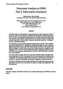
Coverage of clustering on samples.
have a count of 2 - these are: mv1 = h0, 0, 0, 0, 0, 1, ∗, ∗i, mv2 = h0, 0, 0, 0, 0, ∗, 2, ∗i, and mv3 = h0, 0, 0, 0, 0, ∗, ∗, 3i. The remaining 6/8, 7/8 and 8/8 masked shingles that cover the 3 pages each have a count of 1. In the second pass, the 3 8/8 shingle vectors each have a count of 1, and so are processed in an arbitrary order. Suppose we pick them in the order v1 , v2 , v3 . Now, v1 is covered by both mv1 and mv2 with counts 2, and so we select one of them, say, mv1 . Then, the count for mv1 will stay at 2 and the new count for mv2 will be 1 after decrementing by 1. Next, when we process v2 , since mv3 has count 2, it will be selected over mv2 , and the count for mv2 will again be decremented by 1 and the new count for it will be 0. Finally, one of mv1 or mv3 with counts 2 will be selected for v3 . If mv1 is selected, then the count for mv3 will be decremented by 1 to 1. Thus, at the end of the second pass, the counts for mv1 , mv2 and mv3 will be 2, 0, and 1, respectively. And the final clusters at the end of the third pass will be: Cmv1 = {v1 , v3 } and Cmv3 = {v2 }. We need to choose the Web site sample P so that it captures all the interesting large clusters within the site. Our experience has been that large clusters typically have a size greater than max{100, 0.1% of site size}. In our experiments, we have found that taking a 20% sample of a site, with a maximum sample size of 20K, generally enables us to capture all the large clusters within the site. Moreover, pruning all clusters with counts smaller than 20 at the end of the second pass enables us to get rid off the negligible clusters from the sample. (Note that the pruning threshold is always kept at 20 pages independent of the sample size and hence has a minimum value of 0.1% of sample size). 1) Experiments: In order to gauge the effectiveness of our sample size and pruning threshold settings to capture a site’s
large clusters, we perform experiments on daily crawl data for 20 sites. We divide the sites into two categories: large with > 100K pages, and small with between 10K and 100K pages. For large and small sites, we choose random samples of sizes 20K and 2K, respectively, which constitute less than 20% of the site size. The pruning threshold is set to 20 which is 0.1% for large sites and 1% for small sites. Figure 3 plots coverage values for large and small sites. Here, coverage is defined as the fraction of a site’s large cluster pages that are covered by the (masked) shingle signatures of clusters computed using the samples. As can be seen, coverage is mostly above 0.95 for the small sites and above 0.993 for the large sties. Thus, 20% sample sizes and a pruning threshold of 20 are effective at capturing a site’s large clusters. With the above parameter values, in a crawl data set for 436 sites, the average number of clusters per site was 24 with the maximum and minimum being 149 and 1, respectively. B. Page Annotation We learn XSLT extraction rules for each cluster by having human editors annotate a few sample pages from each cluster. Although Web pages within a cluster, to a large extent, have similar structure, they also exhibit minor structural variations because of optional, disjunctive, extraneous, or styling sections. To ensure high recall at low cost, we need to ensure that the page sample set that is annotated has a small number of pages and captures most of the structural variations in the cluster. One simple way to achieve this is to treat each page as a set of XPaths contained in it, and then greedily select pages that cover the most number of uncovered XPaths. A problem with this simple approach is that it considers all XPaths to have equal weight. Clearly, XPaths that appear more frequently across pages in the cluster are more important and thus must have a higher weight. Furthermore, in practice, pages have many noisy sections like navigation panels, headers, footers, copyright information, etc. that are repeated across the pages in the cluster. Intuitively, XPaths in such noisy sections should have a low weight since they cannot possibly contain attribute values that we are looking to extract. On the other hand, XPaths in informative sections of the Web page that contain the attributes of interest should be assigned much higher weights. For an XPath Xi , let F (Xi ) denote the frequency of Xi ; that is, the number of cluster pages that contain Xi . In order to differentiate between informative and noisy XPaths, we assign different weights to them. For this, we leverage the fact that, in a particular Web site, noisy sections share common structure and content, while informative sections differ in their actual content. The informativeness of an XPath Xi is determined as: P ( t∈Ti F (Xi , t)) I(Xi ) =1 − M · |Ti | where Ti denotes the set of content associated with XPath Xi , F (Xi , t) denotes the number of pages containing content
t at the node matching Xi , and M is the number of cluster pages. Intuitively, an XPath Xi in a noisy portion of the page will have repeating content across pages, and thus will end up with a P low informativeness score close to 0 since |Ti | ≈ 1 and t∈Ti F (Xi , t) ≈ M . On the other hand, we will assign a higher informativeness score to an XPath belonging to an informative region that has distinct content across pages; P here, the informativeness score will be close to 1 since t∈Ti F (Xi , t) ≤ M but |Ti | ≈ M . Since we are interested in covering frequently occurring XPaths belonging to informative regions, we assign each XPath Xi a weight w(Xi ) = F (Xi )·I(Xi ). Ideally, we would like our annotation sample to contain pages with the highweight XPaths since these have the attributes that we wish to extract. Thus, for a K size sample, our problem is to select K pages such that the sum of the weights of the distinct XPaths contained in the pages is maximized. This is identical to the maximum coverage problem which is known to be NP-hard, but can be approximated to within a factor of 1 − 1e using a simple greedy algorithm. We can achieve this approximation bound by modifying the approximate greedy solution to order pages based on uncovered XPath weights instead of the unique number of uncovered XPaths as shown in Algorithm 2. Input: Cluster C = {p1 , . . . , pn }, and sample size K; Output: K or fewer sample pages; Initialize the uncovered XPath set X to all distinct XPaths in C, and sample S to ∅; while X 6= ∅ and |S| ≤ K do P Find pi = maxpj ∈(C−S) { Xi ∈pj ∩X w(Xi )}; S = S ∪ {pi }; X = X - {XPaths in pi }; end while return S; Algorithm 2: Weighted greedy algorithm In Vertex, we choose the annotation sample size parameter K = 20. Sample pages are presented to editors for annotation in the order in which they are selected in Algorithm 2. As editors annotate each successive page, an XSLT rule is learnt from the annotated pages so far. If the rule is able to successfully extract attribute values from the remaining pages in the sample, then no further annotations are required. Thus, editors do not need to annotate all the pages in the sample. In fact, our experience over a wide range of Web sites has been that editors typically annotate only 1.6 pages on an average. 1) Experiments: We use the following metrics to evaluate the effectiveness of our proposed sampling approach: 1) Number of samples needed to cover all XPaths. 2) Number of attributes covered by the first sample. We performed our experiments on 10 sites spanning several verticals (product, movie, social networking, etc). Sampling is performed on 400 pages from a cluster within each site. We compared our weighted greedy algorithm with the greedy and random selection schemes. In greedy selection, all
Scheme Random Greedy Our Algorithm
# Sample pages 276.2 24.1 28.2
Attribute coverage 61 64 68
TABLE I C OMPARISON OF SAMPLING SCHEMES .
XPaths have the same weight. In random selection, a randomly selected page is included in the sample set only if at least one of the XPaths in that page is not seen in previously selected pages. Table I depicts the results of our comparison of the various sampling schemes. Covering XPaths: The second column in Table I shows the average number of sample pages needed per site to cover all XPaths in the dataset. This number is 24.1, 276.2, and 28.2 for greedy, random, and our proposed algorithm, respectively. It can be seen that random sampling is not effective. Attribute coverage: The third column in Table I lists the attribute coverage of the first page chosen by various schemes. In the above dataset, the total number of interesting attributes is 69. The number of attributes in the first selected page is 61 with random selection, 64 with greedy selection and 68 with our sampling technique. This demonstrates the effectiveness of our weight assignment function in identifying the pages with rich informative sections. With our algorithm, in 9 out of 10 sites, the first sample covered all attributes. In the remaining site, the inclusion of the second page resulted in the coverage of all the attributes of the site. C. XSLT Rule Learning The annotations in the annotated sample pages AS of a cluster specify the location of nodes containing attribute values. These are used to learn an XSLT rule for extracting attribute values from new pages that map to the cluster. The XSLT rule contains XPath expressions that identify the node in the new page corresponding to each attribute and other components that extract the actual text value of interest from the node. The XPath rules to perform extractions for an attribute are created using structural features on the page. We classify features into two types: strong features and weak features. Strong features are signals that are not expected to change over time. HTML attributes such as class or id, h1 tags, and textual features such as suffix text (“reviews” in “5 reviews”) and preceding text (“Price:” in “Price: $50”) are examples of strong features. Weak features are less robust compared to strong features, and can change frequently over time. Examples of weak features are font and width HTML attributes. Both strong and weak features can be expressed as XPath expressions. Further, we can combine a set of features to form a single XPath expression that selects a set of candidates nodes on each page. We provide details on how features are generated and combined to form XPath expressions in Section III-C.1. In order to extract an attribute, we first try to learn a rule
that precisely extracts the node that contains the value of the attribute using a combination of strong features only. The algorithm described in Section III-C.2 uses a novel Apriori [1] style enumeration procedure to learn the most precise and robust XPath. If such an XPath exists, we call it the pXPath. If a pXPath does not exist, we use an rXPath (which is an XPath having a recall of 1) to generate candidates and then use a Naive-bayes classifier that uses both strong and weak features to select the attribute node. Like a pXPath, the rXPath also uses only strong features, but does not have a precision of 1. We describe how we learn and run the classifier to perform extractions in Section III-C.3. Finally, we incorporate two modules, range pruner and attribute regexes, for selecting the text within the node, and this is described in Section III-C.4. We provide experimental results in Section III-C.5. 1) Feature generation for XPath learning: We denote the set of features generated from an annotated page p with an annotated node a for the attribute of interest as F (a, p) = {(T, l, V )}, where T is the type of the feature, l is the level or distance of the feature from the annotated node, and V is the value for the feature of type T . We generate the following features: Tags: For each node n from the annotated node to the root, we add (“tag”, l,t) as a feature, where l is the distance of node n from the annotated node (0 when n = annotated node) and t is the tag name of the node n. This results in an XPath //t/*/. . ./*/node(). The number of *s in the XPath query is l. id and class: For each node n in the path from the annotated node to the root, if n has an id attribute, we output two features (“id”, l,v) and (“id”, l, ∗), where v is the value of the id attribute. The resulting XPaths for the id attribute are //*[@id=v]/*/. . ./*/node() or //*[@id]/*/. . ./*/node(). We output a similar set of features for the class attribute with type set to “class”. Preceding and following sibling predicates: For each preceding sibling of the annotated node, say the ith preceding sibling, we add (“preceding-sibling-tag-i”, l,t) where t is the tag of the ith preceding sibling. If the preceding sibling has an id attribute, we add (“preceding-sibling-id-i”, l, “ ∗ ”) and (“preceding-sibling-id-i”, l,v). Similarly, we add features if the sibling node has a class attribute. The XPath for this predicate is constructed as //*[preceding-sibling::*[position()=i] [self::t]]/*/. . ./*/node() or //*[preceding -sibling::*[position()=i][@id=v]]/*/. . ./*/ node(). We add a similar set of features for each following sibling as well, with the type set to “following-sibling-tag-i” etc. for the ith sibling. Text predicates: We find the first occurrence of nonempty text to the left of the node and to the right of the node. This text is called anchor text. The text can occur within the node that contains the target text or outside. In the fragment, Our Price: $25.99, let $25.99 be the annotated text and “Our Price:”
is the first non-empty text, and both are within the annotated node under . On the other hand, if the page structure was Our Price: $25.99, then “Our Price:” is the non-empty text to the left of the annotated text but is present outside of the node. When the non-empty text to the left or right of the annotated text is within the annotated node, we call these inside anchor texts. We add the following features for the left anchor text (similarly for the right anchor text). • If the left anchor is an inside anchor, add (“insideleft-word”, 0, w) and (“inside-left-text”, 0, t), where w is the first word to the left of the annotated text and t is the text from the beginning of the node to the annotated text. This is expressed as the XPath query //*[contains( text(), w)] for the word and //*[starts-with(text() , t)] for the text. • If the left text anchor is not an inside anchor, add (“out-left-word”, 0, w) and (“out-lefttext”, 0, t). This results in the XPath fragment //*[preceding::text()[normalize-space(.) != “”][position()=last()][ends-with(., “w”)]1 for the left node and //*[preceding::text()[normalize-space(.) != “”][position()=last()][.=“t”] for full node match. Disjunction of features: We also add disjunction of feature values that have the same type and are at equal distance from the annotated nodes. For example, if the text on the right of the attribute across two annotations are “review” and “reviews” respectively, then we add an additional feature that has a disjunctive value “review” or “reviews”. The corresponding XPath fragment would be //*[ends-with(text(), “review” ) or ends-with(text(), “ reviews” )]. We allow up to 3 values for a disjunction, and we do not add a disjunction feature if the number of values for features with the same type and level have more than 3 values. Note that disjunction features can sometimes overfit to training examples. For example, if for the attribute “Image”, the text on the right is “$12.95”, “$2.95” and “$4.65” on 3 pages respectively, we would create a disjunction feature with the three values. However, a rule created using this feature would extract attributes from the training pages only. In this case, we need another annotation from a page that has a different value for the right text. Since we allow a maximum of 3 values for a disjunction feature, we will not consider a disjunction that takes 4 values. In the worst case, we need 4 annotations for learning a rule for an attribute. Using a disjunction of features has a trade-off between having robust features with disjunctive values (e.g., “review” or “reviews”) and features that overfit to training examples. In our experience, cases of overfitting are few and 1 ends-with is not a supported XPath 1.0 operation, but it can be implemented using string operations.
the benefits of selecting robust features with disjunctive values outweighs the number of cases with disjunctions that overfit to training examples. Combining XPaths for features: Each feature has a corresponding XPath query that selects the annotated nodes, and possibly other nodes. For instance, if (“tag”, 3,div) is a feature, //div/*/*/node() is the corresponding XPath query for the feature. Further, when we combine two or more features, we merge their XPath queries. For example, if (“tag”, 3,div), (“preceding-sibling-class-2”, 3, c1 or c2) and (“id”, 1, i1) are three features that are combined, we can construct an XPath query //div[preceding-sibling::node()[position()=2] [@class=“c1” or @class=“c2” ]]/*/*[@id= “i1 ”]/node(). We denote the XPath corresponding to a set of features, F , as X(F ). 2) Robust XPath Generation: We are interested in generating a robust XPath query (called pXPath) that selects only the annotated nodes and none of the other nodes on annotated sample pages. An XPath is constructed using a combination of features, and our objective is to find the most general XPath (with few features) that will be robust to changes in page structure. We model robustness using two metrics: distance and support. We prefer XPaths with features close to the annotated node over many distant features. Further, we use unannotated sample pages to define the support of an XPath. We prefer XPaths that have support on unannotated pages over XPaths that do not. Given an XPath X, we define prec(X) as the precision of the XPath; i.e. prec(X) is the ratio of the number of correct nodes selected by the XPath and the total number of nodes selected. We define dist(X) to be the maximum distance of the features of the XPath from annotated nodes. And sup(X) is the support of the XPath on unannotated pages. This is the fraction of unannotated pages in which the XPath selects one or more candidates. We expect the XPaths we generate to select all annotated nodes; hence, support on annotated pages is 1. We generate an XPath that satisfies the following properties: 1) The XPath selects all annotated nodes, i.e., recall is 1. 2) Among all XPaths satisfying (1), precision prec(X) is maximum. 3) Among all XPaths satisfying (1) and (2) above, dist(X) is minimum. 4) Among all XPaths satisfying (1), (2) and (3) above, sup(X) is maximum. We use an Apriori [1] style algorithm to generate an XPath satisfying the above 4 properties. Let S be the set of features generated using the feature generation procedure described in the previous subsection. Algorithm 3 starts with XPath candidates C1 , each of which has a single feature from S. In each subsequent iteration we combine features to generate a set of candidates Ck+1 that are more specific than the candidates
Ck considered in the previous iteration. Note that Ck contains candidate sets of features, each set with exactly k features. Let P + be the set of annotated nodes and P − be all other Input: Sample pages (annotated and unannotated), feature nodes on annotated pages. In the k th iteration, we examine set S; candidate XPaths X corresponding to feature sets in Ck , and Output: Maximum precision XPath; prune the XPaths that do not cover all the annotated nodes in P + . We also keep track of the best XPath X seen so far - this C1 = {{f } : f ∈ S}; XPath satisfies properties (1) through (4), that is, it has the k = 1; min dist = ∞; max sup = 0; max prec = 0; minimum dist(X) from among XPaths satisfying properties best XP ath = max prec XP ath = NULL; (1) and (2), and the maximum support from the XPaths while Ck 6= ∅ do having distance dist(X). The best XPath is either stored in Lk+1 = ∅; max prec XP ath (if max prec < 1) or best XP ath (if for all XPaths X(F ), F in Ck do max prec = 1). if X selects all the positive nodes in P + then In order to generate the set of candidates Ck+1 , we store if X selects a negative node in P − or X matches in Lk+1 all the feature sets in Ck that can potentially lead more than one node in an unannotated page then to Xpaths that are superior to the best XPath found so far. Lk+1 = Lk+1 ∪ {F }; Observe that the distance of XPaths is non-decreasing and if (prec(X) > max prec) or the support of XPaths is non-increasing as they become more (prec(X) = max prec and specific in subsequent iterations. Thus, we only add to Lk+1 dist(X) < min dist) or (prec(X) = max prec feature sets whose corresponding XPaths have a precision and dist(X) = min dist and less than 1. Further, we prune from Lk+1 feature sets whose sup(X) > max sup) then XPaths are inferior to the current best XPath in terms of max prec = prec(X); distance and support. The candidates in Ck+1 are then all sets max prec XP ath = X; F containing k + 1 features such that every k-subset of F min dist = dist(X); belongs to Lk+1 . max sup = sup(X); We construct the best XPath query that maximizes precision end if using the enumeration procedure. If the precision is not 1, we else if (dist(X) < min dist) or add a single positional predicate [position()=i] to the (dist(X) = min dist and (sup(X) > max sup)) query for various values of i. If we find one that results in then a precision of 1 while still satisfying property (1), we output best XP ath = X; the final XPath query with the positional predicate. Otherwise, min dist = dist(X); we use the classification framework described in the next max sup = sup(X); subsection. max prec = 1; 3) Classification framework: When the XPath generation end if procedure does not output an XPath with precision 1, we end if select the XPath with the maximum precision and a recall end for of 1. This is called the rXPath. We then use a Naive-Bayes for all XPath X(F ), F ∈ Lk+1 do based classifier to select the correct candidate. We consider if best XP ath 6= NULL and ((dist(X) > min dist) the annotated nodes selected by the rXPath as positive (+) or (dist(X) = min dist and sup(X) ≤ max sup)) examples and other nodes selected by the rXPath as negative then (−) examples. delete X from Lk+1 ; In addition to strong features, we also generate features for end if all HTML attributes and values (not just id and class). We end for do feature selection based on the mutual information of the Ck+1 = {k+1-sets F : all k-subsets of F are in Lk+1 }; features with the labels + and −, and use these features to k = k + 1; build the classifier. Typically, we have many more negative end while examples than positive examples and the number of positive if best XP ath 6= NULL then examples is small (1 − 4 in many cases). If the rXPath has a return best XP ath; precision of 0.1, we will select about 10 nodes per page, out of else which 0 or 1 nodes are positive and the remaining are negative. return max prec XP ath; We employ smoothing to ensure that we do not overfit based end if on a single or few specific features. Algorithm 3: Learn XSLT Rule Features are evaluated relative to the set of nodes generated by the rXPath. Hence, we translate all features that have level 0 to self XPath queries, features with level 1 from the annotated nodes to parent XPath queries, and all features with
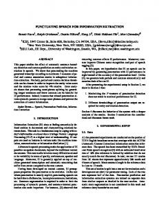
level 2 or above to ancestor XPath queries. For instance, a feature (“class”, 0, c1) is converted to an XPath query on candidate nodes as self::*[@class= “c1”], and a feature (“tag”, 3,div) is converted to ancestor:: div. While performing extractions, we run the classifier on each candidate node and output a winner with the highest + label probability greater than 0.5. 4) Text selection using Range Pruner and Regexes: When the node of interest is selected using the pXPath or the Naive Bayes classifier, we may not be interested in the complete text under the selected node. For example, if the node text contains “Our Price: $25.99”, we need to output “$25.99”. Range pruner is a component that extracts the text of interest from a node or a pair of nodes. It learns the required range information as an offset either from the beginning or the end of the node text, whichever is more consistent. Note that in our example, the string “$25.99” has an offset of 3 from the begining and an offset of 1 from end. In addition to offset-based range selection, we also use regexes for selecting values of “typed” attributes like price (currency + number), phone number, zip code, etc. The regexes are manually created and are associated with the corresponding typed attributes. The regexes both select and validate the attribute values in the presence of surrounding text. 5) Experimental results: We evaluate our rule learning system over 20 large sites from across 3 different verticals, namely, product, business, and forum (such as www.amazon.com and www.epinions.com). These sites typically are script generated and hence have good template structure. The clustering on these 20 sites gave us a total of ≈ 300 clusters. For each cluster, human editors annotated a few pages (maximum of 4 pages) from a sample set and validated the extractions from the rule over a different test set (typically 20 pages). We consider a rule to be valid if it has a precision of 100% and a recall of > 85% over the test set. The attribute-wise precision and recall numbers averaged over clusters are shown in Figure 4. As can be seen in the figure, our system is able to extract attributes with close to 100% precision and > 99% recall for all attributes. A manual inspection of the XSLT rules also showed that the learnt XPaths are robust to structural variations; Table II shows some sample XPaths that were learnt. Note that the rating image XPath for www.cduniverse.com does not have precision 1, and hence we use a classifier to extract the correct node. Weak features such as ancestor::node()[@padding="10px"] and self::node()[@border] help to extract correctly. On a larger scale deployment, we generated rules for 200 sites belonging to product and business verticals. The number of extractions from these sites was around 250 million (65 million from Shopping pages, 85 million from People profile pages, 50 million from Business pages, 50 million from Forum pages). Precision computations on a random sample revealed that the extraction precision is close to 100%. Our system, on an average, required only 2.3 pages to be annotated per cluster, and took 70 msec to extract data from a single page.
Fig. 4.
Attribute-wise Precision and Recall
IV. E XTRACTION S UBSYSTEM The learning subsystem learns a single XSLT rule per cluster within each Web site. Each rule is learnt from a sample of pages belonging to the cluster, and it inherits the shingle signature and the importance score of its cluster. The learnt rules for a site are subsequently used to continuously extract records from additional crawled URLs from the site. In the following subsections, we describe the algorithms employed by the key components of the extraction subsystem in more detail. A. Rule Matching For each crawled page, we need to determine the matching rule and apply it to extract the record from the page. This is done in two steps. We first determine the set of matching rules for the page based on the page URL. The final rule is subsequently chosen based on the page shingle vector. To accomplish the first step, we associate a URL regex with each rule (in addition to a shingle signature). The URL regex has a syntax similar to URLs but is allowed to contain wildcards, e.g., “http://domain-name/product/(.*)/detail.html”. During learning, we select the URL regex for a rule to be the most specific regex that matches all the URLs contained in the cluster for the rule. To prevent overfitting, we impose certain size restrictions on the URL regex. In the first step, we filter out rules whose URL regex does not match the page URL. Then, in the second step, we further narrow down the rules set to those whose shingle signatures match the page’s shingle vector. For a page, there can be more than one matching rule based on the URL regex and shingle pattern. In our experiments, we have found that on an average approximately 2 rules match each page. In such cases, the cluster importance score is used to select the best rule for extraction. Note that using URL regex helps to reduce the number of possible candidate rules for shingle comparisons. Matching a URL to URL regexes is computationally much cheaper compared to computing the page shingle. So for uninteresting pages for which no matching URL regex exists, we can
Domain www.amazon.com www.city-data.com www.alibaba.com www.cduniverse.com www.hotels.com
Attribute price forum title image rating image address
Learnt XPath //node()[@class="listprice"]/node() //td[@class="navbar"]/*/text() //node()[@class="detailImage" or @class="detailMain hackborder"]/*/img //td/img //node()[@class="adr"] TABLE II S AMPLE L EARNT XPATHS
Num Changes 0 1 2 3 4 Total Changes
10% 26 10 5 1 1 27
20% 27 11 4 1 0 22
30% 28 12 2 1 0 19
40% 29 11 3 0 0 17
50% 30 11 2 0 0 15
TABLE III N UMBER OF SITE CHANGE EVENTS AS A
Site
# Clusters
www.alibaba.com www.alibris.com www.amazon.com www.fodors.com www.gsmarena.com www.toysrus.com
6 2 3 10 20 17
# Rule breakage 3 2 3 1 2 1
% URL breakage 100% 99.5% 100% 90.5% 81.8% 80.3%
TABLE IV
FUNCTION OF COVERAGE DROP
THRESHOLD .
S HINGLE TEST STATISTICS FOR RULE MONITORING .
realize significant computational savings by avoiding shingle computation altogether.
Null extractions: If the structure of the XPath pointing to a particular attribute changes with the page’s shingle still conforming to the rule’s shingle signature, then the rule gets applied but the rule application can result in the attribute not getting extracted anymore. • Incorrect extractions: This scenario is similar to the one above except that the rule application results in incorrect extractions. Note that this impacts extraction precision. In order to identify rule breakages, the rule monitoring component identifies 10-20 sample URLs (called bellwether URLs) from each cluster within a site, and crawls them periodically (e.g., daily). The rule monitoring component then performs two kinds of tests on this set of pages: a shingle test and a field test. The shingle test for a rule computes the shingle vectors of the freshly crawled sample pages from the rule’s cluster, and matches the computed shingles with the rule’s masked shingle. If the shingles do not match for a majority of the samples, then the test fails and this signals a change in the Web site structure. The field test captures the two other kinds of coverage drops due to extraction failures. In order to perform a field test, we store the extractions from each sample page at the time of rule creation. As these extractions are correct, we refer to this set of extractions as the golden extractions. The extractions of a freshly crawled sample page (using the rule for its cluster) are compared with the golden extractions. The field test succeeds if all the mandatory attributes are extracted, and the extracted values of constant attributes match between the old and new extractions. A shingle test or field test failure for a rule triggers a site change and causes all the rules for the site to be relearnt. 1) Experiments: Table IV provides statistics on rule breakage for sites. All the sites listed in the table had one or more rule breakages in a one month period. For the first 3 sites, the coverage drop was more than 10% while for the last 3 sites,
B. Rule Monitoring Web sites are dynamic with the content and structure of pages changing constantly. Examples of content changes are price changes, rating changes, etc. Page structure changes can happen due to products going on sale or out of stock, addition of reviews, variable number of ads, etc. These structural changes can result in page shingle changes which in turn can lead to learnt rules becoming inapplicable. We first provide statistics on site structure changes using page shingle changes as a proxy. To characterize site changes, we cluster crawled pages from a site on a given day, and measure the coverage of the clusters on crawl data from subsequent days. Here, coverage is defined as the fraction of crawled pages whose shingle vectors are covered by the shingle signatures of clusters. Any major change in page structure is reflected as a non-negligible coverage drop. We define the site change event as a coverage drop exceeding a certain threshold. Table III provides the number of site changes for 43 sites over the duration of a month (from Dec 20, 2008 to Jan 20, 2009) for different threshold values ranging from 10% to 50%. Row i of the table contains the number of sites that changed i times. It can be seen that several sites changed multiple times over this period. In fact, one site www.amazon.com changed 4 times in one month. The number of unique sites that changed over the 30 day period is 17 (40%) and the number of site changes is 27 (63%). The above coverage-based framework detects only structural changes. But a rule can fail in three different ways: • Shingle changes: Due to changes (minor as well as major) in the Web page structure, the rule might not apply to previously applicable pages, thus resulting in a potential reduction of coverage.
•
the coverage drop was less than 10%. Hence the latter can be considered to be false positives of our rule breakage detection algorithm. The false positives occur because of a change in the number of ads, some frames not fetched correctly, etc. Observe that in the case of false positives, only a small percentage (≤ 10%) of rules break. Further, while almost all bellwether URLs experience shingle changes in the case of genuine site changes, the fraction of bellwether URLs whose shingles change is somewhat lower (80−90%) for false positives. Thus, setting a high threshold for the % of sample URLs broken can help to reduce the number of false positives. C. Rule reuse Two major findings from our rule breakage detection experiments in Section IV-B are: 1) Even minor changes in page structure can cause page shingles to change thereby flagging rule breakage. Approximately 2% of Web sites experience some sort of page structure change each day. 2) Sites undergo partial and not complete changes. For example, for the false positives at the bottom of Table IV, only a small fraction (≤ 10%) of rules break within each site. Hence a site change may be signaled even if only a small fraction of pages within the Web site changes. In these cases, relearning the rules for all the new clusters within a site in the event of a site change may be an overkill, and it may be possible to reuse previously learnt rules for many, if not all, of the new clusters in the site. The candidate rules for reuse are found by calculating the URL overlap between every new cluster with each of the old clusters used to learn the previous rules. Let C be a new cluster and C1 , C2 , · · · , Ck be the old clusters with which C has nonempty URL overlap. Let U = ∪i (C ∩ Ci ) be the URLs in the intersection of C and the old clusters Ci . The matching cluster Ci whose rule we reuse for C is selected using two tests: a shingle test and a field test. Shingle tests for detecting matching cluster pairs C, Ci have two variants. Below, they are listed in decreasing order of strictness. • Cluster match: Clusters C and Ci have the same masked shingle signature. • Page match: The shingles of all the pages in C match the masked shingle signature of Ci . The intuition here is that if Ci and C have similar shingles then we can reuse Ci ’s rule for the new cluster C. In case of ties, we select the cluster with the largest importance score. Let Cm be the matching cluster selected by one of the above two techniques. Then, Rm , the rule for Cm , is subjected to the field test. The field test employs both the old and new versions of the page for every URL in U and is as follows: We apply Rm to the old and new versions of the pages in U . For the field test to be successful, we require that (1) The extracted values for constant attributes should match between the old and new versions of the pages, and (2) Rm should successfully extract all the mandatory attributes from the new version of the pages.
Fig. 5.
Rule reuse results.
If Rm passes the field test, it is associated with C. Otherwise C is scheduled for annotation. 1) Experiments: We performed experiments on 10 sites – 4 sites whose coverage dropped by more than 10% and 6 sites whose coverage loss is very small. The results for the 10 sites are shown in Figure 5 with the 4 sites that had more than a 10% coverage drop listed first. In the figure, we depict the percentage of URLs in new clusters for which an old rule can be reused based on the cluster match shingle test. The results for the two shingle tests were identical on all sites except one (Site 6). Observe that rules can be reused for almost all the URLs from the 6 sites that experienced very small coverage drops. We also plot the sum of the coverage drop and the fraction of URLs for which an old rule can be reused. It can be seen that the sum is close to 1 for most sites. Thus, rule selection is effective since for most sites the fraction of URLs on which reused rules apply is very close to the fraction of URLs that have not changed. In fact, our cluster match method is able to reuse 219 rules out of a total of 352 rules. V. R ELATED W ORK Wrapper learning has attracted a considerable amount of attention from the research community [9], [13], [12], [10], [2], [14], [7]. (See [4] for a recent survey of wrapper induction techniques.) However, to the best of our knowledge, none of the existing research addresses the end-to-end extraction tasks of Web page clustering, rule learning, rule monitoring, and optimized rule relearning. We have also not come across systems that can extract data at Web scale. Early work on wrapper induction falls into two broad categories: global page description or local landmark-based approaches. Page description approaches (e.g., [6], [15], [11]) detect repeated patterns of tags within a page in an unsupervised manner, and use this to extract records from the page. [9], [12] are two examples of supervised landmarkbased approaches. These approaches suffer from a lack of a systematic approach for annotation sample selection and effective wrapper generalization. Another drawback of the previous approaches is that they work on the sequential HTML tag structure thereby missing the opportunity to exploit the underlying DOM structure which provides richer descriptive
power for wrappers. The origins of XPath wrappers can be traced to [14] but the wrappers in this work were hand-created. The wrapper generation technique of Dalvi et al. [7] is closely related to our robust XPath generation algorithm discussed in Section III-C. Like us, [7] also generates robust XPaths through enumeration. However, our approach differs in the following respects: 1. Our XPath enumeration algorithm is based on Apriori [1], and thus generates fewer candidates compared to [7]. 2. The system in [7] models robustness through a tree-edit distance framework and assigns a robustness metric to each feature. This is done for all the identified features. In contrast, our XPath learning algorithm uses only strong features (identified based on domain knowledge) and relies on distance as a metric to generate pXPaths that are robust. 3. If a pXPath does not exist, our system employs a NaiveBayes based classifier with weak features to perform extractions. In this case, even if a single feature is not robust (feature value changes or the feature is removed from the pages belonging to the site), other features in the classifier can help to classify the node correctly. In contrast, XPath rules with weak features will break when that feature changes or is removed from the page. Thus, our classifier based extraction framework is more robust for weak features. 4. Unlike [7], our XPath generation algorithm relies on support from unannotated pages to identify XPaths that are more resilient across a larger set of pages other than training data. 5. Lastly, we consider feature disjunctions to increase the robustness of XPaths. Recently, Zheng et al. [16] proposed wrappers with a “broom” structure to extract records with interleaved attribute values within a page. The broom wrappers include the complete tag-path from the root to record boundary nodes, and hence, may not be resilient to tag modifications. Our wrappers, on the other hand, are general XPath expressions incorporating rich features in the vicinity of attribute nodes; thus, they are likely to be a lot more robust. Unlike wrapper learning, wrapper breakage and repair are relatively less studied. [10] proposes the DataProg algorithm to compute statistically significant patterns (like starting or ending words) for attribute values. A change in the patterns for extracted values then signals that the wrapper is no longer valid. Further, the patterns are searched to find attributes in a page when relearning wrappers. In [5], classifiers use content features (e.g., word/digit count) to label attribute values during wrapper repair. The above works rely primarily on attribute content for verifying and relearning wrappers. In contrast, Vertex uses both page stucture and attribute content for automatically detecting rule breakages and identifying the rules that can be reused. In addition to wrapper induction which requires training data for each site, other techniques requiring less supervision have also been proposed for information extraction. In [17], Conditional Random Fields (CRFs) are trained for each vertical as opposed to each site. Unsupervised techniques in [8] exploit linguistic patterns and redundancy in the Web data for
extraction. These approaches have low precision or recall or both. In contrast, wrapper-based systems can achieve precision close to 100%. VI. C ONCLUSIONS In this paper, we described the architecture and implementation of the Vertex wrapper-based information extraction platform. To operate at Web scale, Vertex relies on a host of algorithmic innovations in Web page clustering, robust wrapper learning, detecting site changes, and rule relearning optimizations. Vertex handles end-to-end extraction tasks and delivers close to 100% precision for most attributes. Our current research focus is on reducing the editorial costs of rule learning and relearning without sacrificing precision. Vertex currently uses page-level shingles for clustering pages and detecting site changes. However, since structural shingles can be sensitive to minor variations in page structure, the total number of rules and rule breakages can be high. We are currently investigating XPath-based alternatives to pagelevel shingles to address both these issues. Unsupervised or minimally supervised extraction techniques like CRFs require less training compared to wrappers but do not have very high precision. We are exploring ways of exploiting site-level structural constraints to boost extraction accuracy. R EFERENCES [1] R. Agrawal and R. Srikant. Fast algorithms for mining association rules. In SIGMOD, 1994. [2] T. Anton. XPath-Wrapper Induction by generating tree traversal patterns. In LWA, 2005. [3] A. Z. Broder, S. C. Glassman, M. S. Manasse, and G. Zweig. Syntactic clustering of the web. In WWW, 1997. [4] C.-H. Chang, M. Kayed, M. R. Girgis, and K. Shaalan. A survey of web information extraction systems. IEEE Trans. on Knowl. and Data Eng., 2006. [5] B. Chidlovskii, B. Roustant, and M. Brette. Documentum ECI selfrepairing wrappers: Performance analysis. In SIGMOD, 2006. [6] V. Crescenzi, G. Mecca, and P. Merialdo. RoadRunner: Towards automatic data extraction from large web sites. In VLDB, 2001. [7] N. N. Dalvi, P. Bohannon, and F. Sha. Robust web extraction: an approach based on a probabilistic tree-edit model. In SIGMOD Conference, pages 335–348, 2009. [8] O. Etzioni, M. Cafarella, D. Downey, S. Kok, A.-M. Popescu, T. Shaked, S. Soderland, D. S. Weld, and A. Yates. Web-scale information extraction in KnowItAll (preliminary results). In WWW, 2004. [9] N. Kushmerick, D. S. Weld, and R. Doorenbos. Wrapper induction for information extraction. In IJCAI, 1997. [10] K. Lerman, S. N. Minton, and C. A. Knoblock. Wrapper maintenance: A machine learning approach. Journal of Artificial Intelligence Research, 2003. [11] G. Miao, J. Tatemura, W. Hsiung, A. Sawires, and L. Moser. Extracting data records from the web using tag path clustering. In WWW, 2009. [12] I. Muslea, S. Minton, and C. Knoblock. A hierarchical approach to wrapper induction. In AGENTS, 1999. [13] I. Muslea, S. Minton, and C. Knoblock. Hierarchical wrapper induction for semistructured information sources. Autonomous Agents and MultiAgent Systems, 1(2), 2001. [14] J. Myllymaki and J. Jackson. Robust web data extraction with XML Path expressions. Technical report, IBM, 2002. [15] Y. Zhai and B. Liu. Web data extraction based on partial tree assignment. In WWW, 2005. [16] S. Zheng, R. Song, J. Wen, and C. Giles. Efficient record-level wrapper induction. In CIKM, 2009. [17] J. Zhu, Z. Nie, J. Wen, B. Zhang, and W. Ma. Simultaneous record detection and attribute labeling in web data extraction. In SIGKDD, 2006.