Web Service for Extracting Stream Networks from DEM Data W. Luo*a, X. Lib, I. Molloyc, L. Dib, T. Stepinskid a Department of Geography, Northern Illinois Univeristy, DeKlab, IL 60115; bCenter for Spatial Information Science and Systems (CSISS), George Mason University, 6301 Ivy Lane, Suite 620, Greenbelt, MD 20770; cDepartment of Computer Science, Purdue University, West Lafayette IN, 47906, dLunar and Planetary Institute, 3600 Bay Area Boulevard, Houston, TX 77058, USA
ABSTRACT Stream networks are important features for hydrologic modeling, geomorphologic analysis of landscape, and many other applications. Automatic extraction of stream network from digital elevation model (DEM) has been implemented in major GIS software such as ArcGIS and GRASS based on flow direction along steepest descent and using some threshold criteria to separate channels and hillslope. However, these hydrology based algorithms often tend to produce results that are spatially uniform, not correctly reflecting the spatial variability in stream dissection patterns. In addition, the traditional paradigm of storing and processing everything on a local machine with locally owned software makes it time-consuming and expensive to process and analyze large quantity of geospatial data, which is often required for Earth System Science research. This paper describes the implementation of a morphology based algorithm for extracting stream networks from DEM data as a Web Service within the framework of GeoBrain, an open, interoperable, distributed, standard-compliant, multi-tier web-based geospatial information services and knowledge building system. This is made possible with recent advances in Service-Oriented Architecture (SOA), geospatial Web Services, and interoperability technologies and allows widest possible accessibility, because the only requirement for the user is an Internet connection and a standard web browser.
. Keywords: Web Service, DEM, stream networks, D8 algorithm, morphology based algorithm, tangential curvature, GeoBrain *
[email protected]; phone (815)753-6828; fax (815)753-6872.
1
1. INTRODUCTION Stream networks are important features for hydrologic modeling, geomorphologic analysis of landscape, and many other applications. Automatic extraction of stream network from digital elevation model (DEM) is quite common and has been implemented in major GIS software such as ArcGIS and Geographic Resources Analysis Support System (GRASS) and specialized packages such RiverTools and TauDEM. These implementations are based on the simple idea that water flows downhill along steepest descent and the algorithms often involve two steps: (1) finding the flow direction (steepest descent) for each cell in the DEM; (2) separating cells that are channel and those that are not based on channelization mechanism and some threshold criteria derived from flow direction. Many variations exist. For step (1), there are D8 algorithm (limiting the steepest descent to 8 cardinal directions, [O'Callaghan and Mark, 1984]) and D¶ algorithm (include all possible directions based on a triangular facet, [Tarboton, 1997]). For step (2), TauDEM actually implemented four different threshold criteria: the contributing area threshold ([O'Callaghan and Mark, 1984]); the stream order threshold ([Peckham, 1995]); the contributing area and the slope threshold ([Montgomery and Dietrich, 1992]); and the contributing area and the stream length threshold. These algorithms (hereafter referred to as hydrology based algorithms) are generally adequate for small scale watershed or in places where there is no significant spatial variation in dissection pattern. However, they tend to create spatially uniform stream networks ([Tarboton and Ames, 2001]) and the selection of proper threshold value for separating channels and hillslopes is often subjective. In addition, large data storage requirement for DEM data and the software license and installation requirement would limit the wide usage of stream networks that can be extracted from DEM. This paper will address the first issue by introducing a morphology based algorithm that has been successfully applied to Mars (which is known for its spatial variation of dissection patterns, [Molloy and Stepinski, 2007]) and Cascade Range, Oregon, USA (where a contrast in dissection also exists, [Luo and Stepinski, 2008]). We will address the second issue by implementing the morphology based algorithm as a Web Service integrated into the GeoBrain system, a Web Service based geospatial knowledge system for providing value-added geospatial service and modeling capabilities to geosciences user community ([Di, 2004]). Since the morphology based algorithm has been reported elsewhere ([Luo and Stepinski, 2008]), we will be brief on the morphology based method and focus more attention on the web service implementation in this paper.
2. HYDROLOGY BASED VS. MORPHOLOGY BASED ALGORITHMS As mentioned in the introduction, the hydrology based algorithms are generally adequate for small scale watershed or in places where there is no significant spatial variation in dissection pattern. However, for large regions where stream dissection pattern is likely to change, the hydrology based algorithms become inadequate. As an illustration of the limitation of the hydrology based algorithm and the advantages of the morphology based algorithm, we have applied both algorithms to a large area in Cascade Range, Oregon, where a contrast in stream dissection pattern exist between the Western Cascades (more dissection, lower elevation, higher local relief) and the High Cascades (less dissection, higher elevation, and lower local relief). The DEM data source for the study area is from the National Elevation Dataset (NED, http://seamless.usgs.gov/), a seamless mosaic of best-available elevation data from different sources, and has a spatial resolution of 37.215 m. Figure 1 shows the general geographic location of the study area and a 3-D perspective view generated from the DEM data showing dissection pattern contrast.
Figure 2(a) is the shaded relief map of the study area illustrating the overhead view of the dissection contrast between Western and High Cascades. Figure 2(b) is the 1:100,000 scale “River Reach Shapefile” (http://www.gis.state.or.us/data/alphalist.html) of the study area, which was originally developed by the United States Geologic Survey (USGS) from either aerial photographs or from cartographic source materials using manual and automated digitizing methods (http://eros.usgs.gov/guides/dlg.html). The USGS river data is known to have accuracy issues (e.g., Morisawa, 1957; Coates, 1958; Mark, 1983), but it constitutes a sufficient ground truth for our purpose, as we are only interested in the algorithms’ ability to extract stream networks that will reflect the general dissection patterns on large spatial scale.
2
Fig. 1. Shaded 3D perspective view of the Cascade Range, Oregon, USA, located between -122.75˚E and -121.31˚E and between 43.31˚N and 45.26˚N. The area is roughly 117×216 km. Blue to orange color ramp indicate elevation from low to high. The Western Cascades (roughly western half of the study area) is characterized by lower elevation but higher local relief and higher dissection density, whereas the opposite is true for the High Cascades (eastern half of the study area).
For the hydrology based algorithms, we used the TauDEM software, which has implemented four different threshold criteria for extracting stream channels ([Tarboton and Ames, 2001]). We have selected the threshold values so that the density of dissection in the western part of the study area is about the same as that of the USGS river data ([Luo and Stepinski, 2008]). Figures 2(c)-2(f) show the results from applying the TauDEM to the study area. Comparing these results with the dissection contrast demonstrated in Figures 2(a) and 2(b), it is obvious that the stream network extracted from the hydrology based method cannot adequately reflect the spatial variation of the dissection present in the study area. The only one that offers a hint of the contrast is the result from slope contributing area threshold (Fig. 2e) because it is known to provide unrealistically higher dissection density for areas having higher local slope (also called “feathering” effect, [Tarboton and Ames, 2001]). However, even this map records the existing contrast much worse than our morphology based method, which is presented below.
3
Fig. 2. Maps showing topography of the study area and results of stream extraction using hydrology based algorithms and morphology based algorithm. (a) Shaded relief map showing the dissection contrast. Black box indicates location of an area shown in Figure 3. (b) USGS river data. (c)-(f) Streams extracted by the hydrology-based algorithm using different channelization criteria as indicated. (g) Streams delineated using the morphology-based algorithm of [Tarboton and Ames, 2001] as implemented in TauDEM. (h) Streams delineated using the morphology-based algorithm of [Molloy and Stepinski, 2007]. See [Molloy and Stepinski. 2007] and [Luo and Stepinki, 2008] for more details.
The idea of using morphology based algorithm to delineate stream networks form DEM is not new ([Peuker and Douglas, 1975; Band, 1986; Howard, 1994; Tarboton and Ames, 2001]). In contrast to the hydrology based algorithm relying mainly on the flow direction, morphology based algorithm delineates the stream networks as parts of the raster having a U-like morphology, which is represented as positive curvature derived from DEM. However, the result is often too sensitive to even the smallest positive curvature, and maps many features that are not proper stream networks. For example, Figure 2(g) is the result from the morphology based algorithm of [Tarboton and Ames , 2001] implemented in TauDEM, which extracted streams that show no dissection contrast in the study area at all.
4
We use a morphology based algorithm that was first developed by [Molloy and Stepinski, 2007] to extract valley networks from DEM on Mars and have been adapted and demonstrated to work well in terrestrial context as applied to a large region in Cascade Range, Oregon, USA ([Luo and Stepinski, 2008]). This algorithm is implemented as a combination of ArcGIS script and C++ programs. More details of the algorithm can be found in [Molloy and Stepinski, 2007] and [Luo and Stepinski, 2008]. Briefly, this algorithm calculates the value of curvature at each cell analytically using a polynomial approximation to the local patch of the surface defined on a 5×5 cells neighborhood centered on a focus cell and then connect the cells with sufficiently large curvature value to form stream networks. This approach solves the over sensitivity to curvature problem of previous morphology based algorithms ([Peuker and Douglas, 1975; Band, 1986; Howard, 1994; Tarboton and Ames, 2001]). The result is shown in Figure 2(h), which delineated stream networks that reflect the dissection contrast in the study area consistent with the visual evidence as shown in Figure 2(a) and the ground truth data as shown in Figure 2(b). More detailed quantitative assessment of accuracy can be found in [Luo and Stepinski, 2008]. Comparing to the hydrology based algorithms, our morphology based algorithm does not require any assumptions about channelization mechanism and correctly delineates streams that are spatially variable over a large region ([Luo and Stepinski, 2008]).
3. BACKGROUND ON GEOBRAIN AND WEB SERVICE Traditionally, scientific analysis of geospatial data, such as extracting stream networks from DEM, takes place at scientists’ local machines with local data collection and software. This requires researchers to have large local storage devices and necessary software licenses purchased and installed. In addition, researchers also have to spend significant amount of time to preprocess the data so that they are in proper format and projection to be brought into the software packages. This paradigm, everything locally owned and operated, makes analysis and application of geospatial data very expensive and time-consuming (Di, 2007). Recent advances in Service-Oriented Architecture (SOA), geospatial web services and interoperability technologies have made it possible for researchers to access data residing on a remote server without having to download them physically to their local machine and to string Web Services available over the Internet together to complete their own analysis tasks, i.e., shifting to a Web-and-Service-Centered paradigm (Di, 2007). A Web Service is defined by the World Wide Web Consortium (W3C) as "a software system designed to support interoperable Machine to Machine interaction over a network." GeoBrain is a Web Service based geospatial knowledge system for providing value-added geospatial service and modeling capabilities to geosciences user community (Di, 2004). Funded by NASA, GeoBrain is developed to make petabytes of NASA’s Earth Observing System (EOS) data and information as easily accessible as possible to higher-education users, both professors and students. In other words, through the Open GIS Consortium (OGC) standard compliant Web Services in GeoBrain, users can not only easily access NASA data as if the data are residing on their local machine, greatly streamline the preprocessing, but also access necessary tools or building blocks to build tools to analyze large amount of geospatial data. GeoBrain has ported many of the functions of the open source GIS software Geographic Resources Analysis Support System (GRASS) (Di, 2004; 2007). Taking advantage of the existing infrastructure of GeoBrain, the Web Service for morphology based stream extraction from DEM data is implemented as part of the GeoBrain and incorporated into the Web Service-based Online Analysis System (GeOnAS, http://geobrain.laits.gmu.edu:8099/OnAS/), a fully extensible online analysis system for using GeoBrain Web services to discover, retrieve, analyze, and visualize geospatial and other network data. With this implementation, all that needed for the user is an Internet connection and a standard web browser, which is readily available nowadays.
4. IMPLEMENTATION OF MORPHOLOGY BASED ALGORITHM AS A WEB SERVICE IN GEOBRAIN The actual implementation of stream extraction Web Service is written in Java, which calls some basic programs including pit filling corrections, flow direction computation, flow accumulation computation ([Tarboton and Ames, 2001], http://www.neng.usu.edu/cee/faculty/dtarb/tardem.html#Installation), the original morphology based algorithm ([Molloy and Stepinski, 2007]) and some utility functions ported from GRASS GIS. The algorithm programs are mainly written in C++, and partly in FORTRAN. All programs are compiled and linked by C++ compiler and FORTRAN
5
compiler on GeoBrain Platform. Because many GRASS commands can be called within the scripts ([M. Neteler and H. Mitasova, 2004]), we just need to write codes to combine external executables and a few lines of GRASS shell scripts and other utility programs to perform stream extraction tasks. The requisite environment variables are also set in the scripts. The exec() method of java.lang.Runtime class is used to call external programs or commands from within a Java program. The following workflow is involved to derive stream network from DEM using morphology based algorithm: 1) Getting DEM data: The Web Service is designed to accept and save DEM data from any URL pointing to the DEM data. This provides more flexibility for data transfer in different servers. The service works with DEM data in GeoTIFF format. 2) Filling DEM data: Execute the flooding algorithm program. The input data need to be in ESRI ASCII grid format and the output is a pit filled elevation data file. Here we call GRASS functions to convert data format. 3) Computing flow direction: Execute the D8 flow direction algorithm program. This will generate D8 flow directions and D8 slopes for each grid cell. Steps 2) and 3) are necessary for step 6). 4) Calculating tangential curvature: Execute morphology based algorithm program. This program takes elevation data file and calculates curvature analytically using a polynomial approximation to the local patch of the surface defined on a 5×5 cells neighborhood centered on a focus cell. 5) Thresholding tangential curvature surface: The curvature threshold is a value above which a cell will be considered as having U-shape morphology. We make this threshold as a command line argument that could be passed into the executable through the Web Service interface, thus user could supply this value. The result of this step is a grid of network segments composed of cells with U-shaped morphology. 6) Computing flow accumulation: Execute the flow accumulation algorithm program. This program takes network segments (resulting from step 5)) as weight, so only cells with the U-shaped morphology will contribute to the flow accumulation. The result of this essentially connects stream segments into an integrated stream network imbedded in the flow accumulation grid. 7) Thresholding flow accumulation: Call GRASS functions to import the above flow accumulation grid into GRASS environment and use GRASS map algebra to threshold it to form the stream network. The flow accumulation threshold variable is also defined as an input parameter of the web service that user can change. 8) Thinning the result grid to get final network: Execute GRASS thinning algorithm so that width of the stream is only one cell. 9) Export the result of connected streams in different formats: Resulting streams could be exported as GeoTIFF, TIFF and ESRI_shapefile format by converting them from GRASS format. The stream extraction service interface is defined using Web Services Description Language (WSDL). A WSDL file describes what operations and data structures are available for the service. We define the request parameters and response parameters as complex data types in WSDL file. The above mentioned variables, such as DEM data URL, curvature threshold, flow accumulation threshold, resulting output format, and output GeoTIFF file type if resulting output format is specified as GeoTIFF, are passed to the web service definitions. The service will respond with a resulting stream URL and a string message about result format. The documentation elements which contain the descriptions for the service, operation and each parameter are added in the WSDL. They could be parsed and explained to the users through GeOnAS. The stream extraction Web Service is deployed in a server like Tomcat with AXIS, which is a toolkit for deploying and using Web Services and is an open-source implementation of Simple Object Access Protocol (SOAP). The advantage of using AXIS is that developers and users do not need to learn SOAP or other low-level Internet protocols. To access stream extraction Web Service, a Web Service client is needed. The stream extraction Web Service is registered into GeoBrain’s Catalog Service for Web (CSW) so that it could be searched and invoked by GeOnAS toolkit. GeoOnAS allows the user to search DEM data, invoke stream extraction service to directly process the found DEM data, and obtain stream networks result via a URL link, all through GeOnAS in a standard web browser such as Internet Explorer or Firefox, without the user needing to download and install any new software, or to learn how the service actually performs its tasks ([Di et al., 2007]).
6
5. INTERFACE OF WEBSERVICE AND ITS USAGE Since the morphology based stream extraction algorithm is implemented within the framework of Web Service-based Online Analysis System (GeOnAS), a fully extensible online analysis system for using GeoBrain Web services to discover, retrieve, analyze, and visualize geospatial and other network data, we can search for DEM data over the Web and run morphology based Web Service to obtain the result in a one-stop visit to the GeOnAS website http://geobrain.laits.gmu.edu:8099/OnAS/. The following briefly describes the major steps involved and what the interface looks like.
1). Creating a new project The first step is to create a new project by selecting “New project” command in the File menu or by clicking on the shortcut button on the toolbar. The spatial reference system and geospatial bounding box of an analysis region of interested is specified by either selecting the place from a dropdown box or directly entering geographic coordinates.
Fig. 3. GeOnAS interface for creating a new project by specifying study area geographic bounding box.
2). Adding DEM data The next step is to add the DEM data by clicking on “Add New Layer” button on the toolbar. This action will pop-up a dialog-box with two options “raster” and “vector” for data format. Choose “raster” for analyzing DEM data. The catalog services are now invoked.
Fig. 4. GeOnAS interface for adding raster data set to the project map window.
7
3). Searching DEM data We can search various remote sensing data products (Landsat data, MODIS data, ASTER data, etc.) from both GMU CSISS local catalog and NASA ECHO. There are some search criteria that allow the user to specify data time range, collection range and other attributes such as Collection, Instrument Name, Platform Name, Topic Keyword, and Archive Center. Submitting query request, datasets matching search criteria will be shown in the search window. The selected data could be added into GeOnAS and displayed on its map panel. The user could specify data resolution, width and height by Web Coverage Service (WCS).
Fig. 5. GeOnAS interface for searching SRTM DEM data.
4). Invoking stream extraction web service Now we can use the menu “Web Service” to invoke stream extraction service which has been registered in our CSW (Catalog Service - Web Profile). The operation “curvatureBasedMethod” implements morphology based algorithm. The required values for request parameters are:
Fig. 5. GeOnAS interface for invoking morphology based stream extraction Web Service.
8
sourceURL: URL of searched DEM data. This can be added directly by selecting the data in left data panel. tcurv_threshold: threshold tangential curvature (Float type). flowaccm_threshold: threshold flow accumulation (Integer type). outputFormatType: Format of output file. Three options: GeoTIFF, TIFF and ESRI_Shapefile. The default value is specified as GeoTIFF. outputGeoTiffType: Type of output GeoTIFF file if outputFormatType is specified as GeoTIFF. Options: Byte, Int16, UInt16, UInt32, Int32, Float32, Float64, CInt16, CInt32, CFloat32, CFloat64. The default value is specified as Byte. Here the users could click question mark to get the description of each parameter which is parsed from WSDL. The stream extraction task is submitted to the server by clicking on the “Invoke” button. The running status of this task will be displayed in left “task” panel. GeOnAS could invoke a Web Service asynchronously. After invoking a Web Service, the users do not need to wait for the responses. They can continue other work; they can even save and close the current project and handle the responses later on. This option is especially useful for users having to process large DEM data.
5). Viewing the results When the submitted task runs successfully, the responses would return in a pop up windows. Result data can be added into the GeoOnAS for view and can be downloaded to the user’s local machine. The user could also check his or her email to get the responses from uncompleted task in his or her saved project. We can see that three inputs control the stream results: resolution of DEM data, curvature threshold and flow threshold. It is very easy to change these variable values to run the algorithms through GeOnAS, and very convenient to compare the results visually in this system. Figure 6(a) shows a screen capture of the result from applying the morphology based stream extraction Web Service to the boxed area shown in Figure 2(a), which correctly reflects the contrast in dissection pattern as visually seen in Figure 2(a). For comparison, we also applied the hydrology based stream extraction Web Service based on ported GRASS functions using contributing area threshold to the same boxed area and the result is shown in Figure 6(b). Clearly, the hydrology based algorithm generated a uniformly distributed stream network that does not reflect the spatial contrast of dissection as shown in Figure 2(a).
(a)
(b)
Fig. 6. (a) Result from morphology based stream extraction Web Service for the boxed area shown in Fig. 2(a), showing dissection pattern consistent with visual evidence as shown in boxed area in Figure 2(a). (b) Result from hydrology based stream extraction Web Service based on ported GRASS functions using contributing area threshold. The pattern of the resultant stream networks are spatially uniform, not consistent with visual evidence as shown in the boxed area in Figure 2(a).
9
6. CONCLUSION AND FUTURE WORK Hydrology based algorithms for extracting stream networks from DEM data generate spatially uniform results, not reflecting the true spatial variation in stream dissection pattern, as demonstrated in Cascade Range, Oregon, USA. We have developed a morphology based Web Service within the frame work of GeoBrain, which not only is able to delineate streams that correctly reflect the spatial variation of dissection pattern, but also is readily accessible to anyone with an internet connection and a standard Web Browser. We are currently working on improving ease of use of the interface, writing documents and tutorials, and improving the efficiency of the algorithm so that larger dataset can also be processed quickly without having to wait in asynchronous mode.
REFERENCES 1
Band, L.E., Topographic partition of watersheds with digital elevation models, Water Resources Research, 22 (1), 15-24, 1986. 2 Coates, D.R., 1958. Quantitative geomorphology of small drainage basins in southern Indiana. Technical Report 10, Office of Naval Research Project, Department of Geology, Columbia University, NR, 389-1042. 3 Di, L., 2004. GeoBrain-A Web Services based Geospatial Knowledge Building System. Proceedings of NASA Earth Science Technology Conference 2004. June 22-24, 2004. Palo Alto, CA, USA. (8 pages. CD-ROOM). 4 Di, L., P. Zhao, W. Han, Y. Wei, and X. Li, Web Service-based GeoBrain Online Analysis System (GeOnAS). in NASA Science Technology Conference 2007, 19-21 June 2007., University of Maryland, College Park, MD, 2007. 5 Howard, A.D., A detachment-limited model of drainage basin evolution, Water resources research, 30 (7), 2261, 1994. 6 Luo, W., and T.F. Stepinski, Identification of geologic contrasts from landscape dissection pattern: An application to the Cascade Range, Oregon, USA, Geomorphology, in press, 2008. 7 Mark, D.M., 1983. Relations between field-surveyed channel networks and map-based geomorphometric measures, Inez, Kentucky. Annals of the Association of American Geographers 73, 358–372. 8 Molloy, I., and T.F. Stepinski, Automatic mapping of valley networks on Mars, Computers & Geosciences, 33 (6), 728-738, 2007. 9 Montgomery, D.R., and W.E. Dietrich, Channel Initiation and the Problem of Landscape Scale, Science, 255 (5046), 826-829, 1992. 10 Morisawa, M., 1957. Accuracy of determination of stream length from topographic maps. Transactions of the American Geophysical Union 38, 86-88. 11 Neteler, M., and H. Mitasova, Open Source GIS: A GRASS GIS Approach, 424 pp., Kluwer Academic Publishers, Boston, Dordrecht, 2004. 12 O'Callaghan, J.F., and D.M. Mark, The extraction of drainage networks from digital elevation data, Computer Vision, Graphics and Image Processing, 28, 323-344, 1984. 13 Peckham, S.D., Self-Similarity in the Three-Dimensional Geometry and Dynamics of Large River Basins, PhD Thesis thesis, University of Colorado, 1995. 14 Peuker, T.K., and D.H. Douglas, Detection of surface-specific points by local parallel processing of discrete terrain elevation data, Computer Graphics and Image Processing, 4, 375-387., 1975. 15 Tarboton, D.G., A new method for the determination of flow directions and upslope areas in grid digital elevation models (Paper 96WR03137), Water resources research, 33 (2), 12, 1997. 16 Tarboton, D.G., and D.P. Ames, Advances in the mapping of flow networks from digital elevation data, in World Water and Environmental Resources Congress, ASCE, Orlando, Florida, 2001.
10