bear this notice and the full citation on the first page. To copy otherwise, to ... points, and to create a web based visualization infrastructure that uses the user's ...
Webcams in Context: Web Interfaces to Create Live 3D Environments Austin D. Abrams, Robert B. Pless
∗
Department of Computer Science and Engineering, Washington University in St. Louis Saint Louis, Missouri, United States
ABSTRACT Web services supporting deep integration between video data and geographic information systems (GIS) empower a large user base to build on popular tools such as Google Earth and Google Maps. Here we extend web interfaces designed explicitly for novice users to integrate streaming video with 3D GIS, and work to dramatically simplify the task of retexturing 3D scenes from live imagery. We also derive and implement constraints to use corresponding points to calibrate popular pan-tilt-zoom webcams with respect to GIS applications, so that the calibration is automatically updated as web users adjust the camera zoom and view direction. These contributions are demonstrated in a live web application implemented on the Google Earth Plug-in, within which hundreds of users have already geo-registered streaming cameras in hundreds of scenes to create live, updating textures in 3D scenes.
(a)
General Terms Algorithms
Categories and Subject Descriptors I.4.1 [Image Processing and Computer Vision]: Digitization and Image Capture—imaging geometry; I.4.9 [Image Processing and Computer Vision]: Applications; H.2.8 [Information Systems]: Database Applications—spatial databases and GIS
Keywords Camera calibration, geospatial web services, participatory GIS, pan-tilt-zoom cameras, social computing, voluntary geographic information, webcams
∗email: {abramsa, pless}@cse.wustl.edu
Permission to make digital or hard copies of all or part of this work for personal or classroom use is granted without fee provided that copies are not made or distributed for profit or commercial advantage and that copies bear this notice and the full citation on the first page. To copy otherwise, to republish, to post on servers or to redistribute to lists, requires prior specific permission and/or a fee. MM’10, October 25–29, 2010, Firenze, Italy. Copyright 2010 ACM 978-1-60558-933-6/10/10 ...$10.00.
(b) Figure 1: (a) A subset of images taken from a pantilt-zoom camera. (b) An automatically-generated geo-registered panorama in 3D within a web app (shown with an off-white border). Calibration of the camera with a few user correspondences permits placing these images in correct geographic context.
1.
INTRODUCTION
The world wide web has an increasingly large, diverse, and interesting set of sensors that provide live updates. While many projects have worked to integrate this sensing data within GIS (and to provide frameworks for querying and visualizing this data), they typically represent streaming video sources as “just another sensor”. However, to interpret camera data automatically, it is often vital to know not just where the camera is, but also its orientation and camera zoom. This paper seeks to address this problem within the context of organizing all publically available webcams so that they can be used as visual sensors. The geometric constraints required to register imagery to GIS are well known. However, there are several challenges in
effectively calibrating all cameras. Fully automated systems for geo-calibrating and geo-orienting cameras [8, 7, 17, 12] report geo-location accuracy to the scale of miles, and orientation accuracy to a scale of degrees, which is insufficient to map pixel data onto 3D models. Thus, we believe that in the foreseeable future, human assistance will be necessary to provide sufficient calibration. Second, webcams are emplaced by a large collection of different organizations, from private citizens to national parks to businesses of all sizes, and most cameras do not publish accurate calibration information. Third, a recent non-exhaustive count [6] has found URLs for more than 17 000 webcams. Thus we seek to create tools which make it simple for arbitrary users on the web to contribute to calibrating all the worlds cameras. We create a web application allowing anyone to calibrate cameras by specifying a few corresponding points, and to create a web based visualization infrastructure that uses the user’s web browser to perform all the necessary image warping. This eliminates the need for any central organization to be responsible for geo-calibrating cameras, and makes the system scalable to the large number of cameras by not requiring a central server to touch the live video data. Previous work [1] defined a start to this process; showing a web interface which allows one to map polygons in a webcam image to polygons in either Google Maps or Google Earth, to infer the camera calibration, and to show live views with those polygons updating from the live feed. There are two major contributions of this paper. The first is to more explicitly reason about streaming video data from a camera that is geo-calibrated. We give an algorithm which maps every image pixel onto the 3D scene structure, and show how to use the extra depth information to aid a user who may only want to use part of the image data to retexture the 3D model. Second, a large number of the most popular cameras, and those that may benefit most from giving the images a context with respect to a 3D model, are pan-tilt-zoom (PTZ) cameras. Web interfaces allow many PTZ cameras to be controlled remotely through a web interface, so to map the image data onto the 3D scene, the camera orientation and zoom need to be updated dynamically. To support this, we discuss methods of solving for the calibration parameters from a small set of points clicked under different viewing directions and show our interface where a user can remotely move the physical camera and watch a virtual, textured camera frustum move to mimic the camera motion.
2.
RELATED WORK
Creating systems to support the organization, querying, and data integration from distributed sensors with known geo-location has been a major focus of work over the last decade. Classic works include IrisNet [4] and SenseWeb [13, 9], which offer frameworks to organize, collect, filter, and combine sensor feeds, to enable distributed queries with reasonable response times. However, these architectures leave a centralized datahub responsible for collecting data, which makes it difficult for them to deal with large sets of video feeds. There have been several other efforts integrating video into a 3D context. Most recently, Kim et al. [10] describe methods to add dynamic information into virtual earth environments, by displaying multiple video streams in a single context. They provide compelling results by merging several
video streams into a view-dependent texture that minimizes artifacts of viewing a back-projected texture from extreme angles. Sawhney et al. [15] provided the first instance of projecting textures onto a geo-referenced space in the Video Flashlights system, which places several cameras from a network in a single 3D context. Sebe et al. [16] extends this topic by implementing a multi-camera tracking system for surveillance purposes, integrated within a geospatial context, and Gliet et al. [5] create a GIS-mashup that maps weather data onto the sky part of a webcam image (but ignores the part of the scene below the horizon). A previous paper [1] developed an interface designed so that the camera registration and scene view process is approachable for novice users. The authors show that the userbase creates scenes with great internal consistency and overall quality. Millions of photographs have been annotated with a single latitude and longitude, which offers a wealth of opportunity for geographic analyses. These geotags have been used to make maps, annotate GIS applications, find oftenphotographed landmarks across the world, and find common photographic ‘circuits’ through urban environments [3]. In [11], Kopf et al. use an image annotated with the geolocation and orientation of the camera, as well as the 3D geographic coordinates of every pixel in the scene to dehaze, relight, and annotate images. In this paper, we simplify the interface necessary to complete this type of registration and consider applications of this to live imagery. In [14], Sankaranarayanan and Davis demonstrate a registration framework for a network of PTZ cameras. They use a spherical ‘fisheye’ panorama to register a PTZ camera to a common geographic space through an affine transformation. They use this geographic space to coordinate the network of cameras and track objects across the different cameras in the network. Although we use a different calibration approach, the motivating ideas and problem statements are similar. In this paper, we show a PTZ registration and calibration framework for a single camera that relates the parameters of a movable camera in terms of familiar camera models from computer vision. Furthermore, we extend the work of Sankaranarayanan and Davis by incorporating geographic altitude and the effects of zooming the camera on the resulting image.
3.
GEO-INTEGRATING STILL WEBCAM IMAGES
Previous work [1] gives an initial implementation of a system for integrating live webcam feeds within 3D GIS applications (such as Google Earth) and 2D GIS applications (such as Google Maps). In this section we follow their notation to present the basic geometric constraints relating the webcam image to geographic coordinates in order to give background for the contributions we offer in the next section.
3.1
Interface
Towards the integration of webcams into a 3D geographic space, we require a user to find a webcam and click on a small set of correspondences between the image and the 3D GIS data. The correspondences can be defined as a single point, a triangle, or a quadrilateral. The latter two cases are automatically textured in order to view the live 3D scene.
(a)
(b)
(c)
Figure 2: The user input process to register static webcams. (a) The user drags markers across a 2D webcam image, and then (b) creates a correspondence between the 2D image and the 3D geographic space by dragging 3D markers to match the 2D points. (c) A polygon with live textures is created and displayed to the user. Users repeat this process until the scene is sufficiently covered.
A brief description of the user input process is given in Figure 2.
find K and R, and we get T as
m14 T = −R m24 . m34 !
3.2
Camera Calibration
When a user provides sufficient correspondences, the full 3D camera calibration is computed. Camera calibration is a well-known problem: given a set of points on an image (xi , yi ) that correspond to some set of known 3D locations (Xi , Yi , Zi ), find a 3 × 4 projection matrix M such that Xi xi w Yi yi w = M Zi w 1
(1)
where w is an arbitrary homogenous scaling factor. The known 3D locations (Xi , Yi , Zi ) are computed by converting the (latitude, longitude, altitude) coordinates of the selected correspondences into a normalized Cartesian space. Six linearly independent correspondences between image space and 3D space are sufficient in order to calibrate the camera using least squares. We require 12 correspondences in order to avoid formal ambiguities caused by users choosing all points from one large planar surface, and to overconstrain the system to help recover from small misregistrations. Then, M can be decomposed into an intrinsic 3×3 camera matrix K, a 3×3 rotation matrix R, and a translation vector T: M = K[R|T ]
fγ K= 0 0
s f 0
x0 y0 . 1
Here, f is the focal length of the camera, γ is the aspect ratio of the image, s is the skew of the camera, and x0 and y0 denote the principal point of the image, usually in the center. We find M using the user defined corresponding points and linear least-squares solution to Equation 1. Denoting the i, j th element of M as mij , we use the QR decomposition to
The rotation matrix is further decomposed into its three constituent Euler angles, and these are converted into the heading, tilt, and roll of the camera. The translation vector T is then converted back into geographic coordinates. Thus, at the conclusion of this process the latitude, longitude, altitude, heading, tilt and roll of the camera are all known in the coordinate system of the 3D GIS data. Furthermore, since the camera calibration is known, we know which ray in space each pixel in the image looks along.
4.
UTILIZING DEPTH INFORMATION FROM GIS
Given the complete calibration of a camera relative to a 3D scene model, it is possible to annotate each pixel of the image by exactly what geographic point on the scene is imaged by that pixel.
4.1
Automatic Scene Generation
In order to texture the scene a static camera covers, we require the user to mark off sections of an image and register them to the 3D environment. However, once a camera is accurately calibrated, the transformation that maps the 3D structures and terrain in a scene to an image is known. If the geometry of the scene is also provided (in our case, through the buildings and ground altitude provided by Google Earth), then the mapping for the rest of the scene can be automatically completed. To automatically generate a scene, we follow these steps. 1. 2. 3. 4.
Generate image annotated with geotags for each pixel. Triangulate set of georeferenced 3D points. Remove triangles that cover depth discontinuities. Texture the mesh using camera calibration.
Given the fully geo-calibrated camera for which we know the projection matrix M , we can solve for the potential
(a)
(b) Figure 3: (a) An image from a webcam calibrated through the web interface. (b) The automaticallygenerated polygons and live textures from the calibrated camera in the context of the geometry provided in Google Earth, shown with a violet border.
points Q on the ray that pixel (x, y) views: xw − m14 m11 m12 m13 yw − m24 = m21 m22 m23 Q w − m34 m31 m32 m33
(2)
Here, w is the arbitrary homogenous scaling factor. From here, we use GIS-provided methods to find the intersection of this ray into the scene’s geometry. We repeat this process for every (x, y) to generate a full depth map. In most images of outdoor scenes, there can be large depth discontinuities between two adjacent pixels, where the geometry of the scene abruptly changes (such as the edge of a building). Although the pixels themselves are very close, the locations of their corresponding 3D points can be drastically different. A simple triangulation of the scene therefore results in triangles with very long edges, where a triangle crosses a depth discontinuity boundary. However, if the background of an image has a cohesive structure (such as a mountain), then it is expected for two adjacent pixels in an image to be somewhat far away, even if there is no depth discontinuity. In other words, the further away an object is, the 3D distance of two adjacent pixels on that object should inherently increase. To prune only the triangles with high depth discontinuity, we score each triangle based on its depth from the camera and the length of its longest edge. For some triangle P QR where the vertices have depth dP , dQ , and dR , we give the triangle a score sP QR as: sP QR =
max($P − Q$, $Q − R$, $R − P $) dP + dQ + dR
This score will be high for any triangle that has long edges but is close to the camera (and is likely a depth discontinuity), but it won’t adversely score cohesive distant elements that have inherently long edges. In practice, we remove all edges that are 10% of a standard deviation above the median score. Figure 3 shows an example scene where the live textured mesh has been automatically created from the calibration of the webcam and the geometry provided by the GIS application. Thus, through a web interface, a user can provide a small set of correspondences (at least twelve) between an image and the geographic scene from which the system will automatically perform camera calibration. Given known scene geometry (provided by GIS applications), this calibration provides the transformation required to retexture a large and complicated scene. In the previous system, users would have to provide a large number of correspondences related to the complexity of the scene geometry. This is particularly useful for scenes in which the geometry of the scene is not planar. For example, Figure 4 shows a scene in which the side of a mountain range has been mapped with a live texture. If this scene were to have been created manually, the user would have had to create several thousand correspondences by hand. In practice, supplying the necessary set of correspondences through the web interface is fast. Calibrating a new camera usually takes between 5 and 30 minutes, depending on user experience and the density of existing geometry within Google Earth. Our registration database contains 94 scenes which have enough correspondences to be calibrated. Of these, 48 have an average pixel reprojection error less than 10 pixels, which is accurate enough to reliably retexture large portions of the scene automatically.
4.2
Calibration-Assisted Scene Model Creation
The full automation creates very complicated scene geometry, and may define updating textures for regions of the scene which are poorly captured by the video feed or otherwise uninteresting. For example, pixels in the far background are often averages over large spatial areas, and become gray and non-descript. These portions of the scene add nothing to the geometric understanding of a scene. Furthermore, during informal observation of users, we have found that registering points in a 3D geographic space is challenging for novice users, who may be inexperienced with manipulating objects in a 3D environment. While a user may be used to moving 2D objects around the screen (as they must do when specifying correspondences on a webcam image), moving 3D points with 2D mouse controls is challenging. Once the camera is calibrated, we allow users to take advantage of the geometry in the scene to aid the 3D point manipulation process. As users drag a 2D point around the calibrated webcam image, the corresponding 3D point moves to its most likely 3D location, effectively eliminating user manipulation for the 3D case. This calibration-assisted interface solves both the issue of manipulating objects in a 3D environment and creating contextually-significant meshes in the foreground of webcam images. For any calibrated camera, the relationship between 3D world coordinates and image coordinates is known. Any 2D image point (x, y) in the image has an associated ray
(a)
(b)
Figure 4: (a) The terrain and satellite model for a mountain viewed through Google Earth. (b) A part of the automatically-generated mesh, using the textures from a live webcam. Creating this mesh by hand would require a user to submit tens of thousands of perfectly-aligned correspondences.
in space (defined by Equation 2), so we intersect that ray with the 3D scene geometry and place the corresponding 3D geographic point there. However, this assumes that the initial calibration has been done correctly and the underlying geometry of the scene is consistent with the webcam image. We allow the user to adjust the geolocations of the 3D points if either of those assumptions fail. Figure 5 illustrates how calibration-assisted registration offers an intuitive, accurate alternative for novice users to create live textured meshes of a scene. In future work, we anticipate that more geometric constraints will provide useful interface tools. For example, from the calibration of the camera, for any pixel, we can find the ray that contributes to that pixel, as in Equation 2. If the camera has been calibrated correctly, the corresponding 3D point must lie somewhere along that ray. If we constrain the user to place the 3D point somewhere on this ray, then the user only has one degree of freedom while manipulating a 3D point. This kind of geometric constraint would be useful in rural areas, where 3D buildings may be lacking or out-of-date, but there are enough correspondences available from satellite imagery to accurately calibrate a camera.
5.
GEO-INTEGRATING PAN-TILT-ZOOM WEBCAM IMAGES
We next consider the problem of the automatic calibration and dynamic viewing of popular PTZ cameras into virtual geographic environments. Typically, PTZ cameras have an interface where any user can remotely rotate or zoom the physical camera. PTZ cameras are ideal for surveillance, since one camera can cover a very wide field of view, but still zoom to get high-resolution images. With dynamic cameras, geographic context is especially important. Even if a PTZ camera has been placed near easily-recognizable landmarks, arbitrary users can easily rotate and zoom the camera into geographically uninteresting locations. Therefore, understanding the geographic position and orientation of any view in the camera’s range is critical
in attempting to understand the geometric foundations of the scene. In the following sections, we describe a camera model that responds to variations in rotation and focal length, and show how we calibrate such a camera given a set of correspondences. Figure 1 shows a collection of automatically-oriented polygons in a panorama, where the position and orientation is given by the calibration of this camera model. In order to represent a correspondence between a point on a pan-tilt-zoom camera and its environment, we collect an image point, a 3D geographic point, and the current pan, tilt, and zoom of the camera. We gather this metadata from PTZ cameras that offer a supplementary information file that contains, among other things, the current pan, tilt, and zoom of the camera, in an arbitrary but bounded scale. As before in Equation 1, we assume that some 3D point (Xi , Yi , Zi ) projects onto an image point (xi , yi ) through a 3 × 4 matrix M . However, since this matrix is dependent on the camera’s rotation and zoom, we now represent this relationship as: Xi xi w yi w = M i Y i Zi w 1 where Mi is a function of the pan, tilt, and zoom of the camera at the time the image was taken, denoted as pi , ti , zi . Here, we assume that pi and ti are in radians, and that zi ∈ [0, 1], where z = 0 and z = 1 represent the camera at its smallest and largest focal lengths (fully zoomed out and fully zoomed in), respectively. Then, we can represent Mi as a function of the matrices Ki and Ri , the intrinsic camera matrix and the camera’s rotation matrix for correspondence i: Mi = Ki [Ri |T ]
(3)
Notice that, because the position of the camera never changes, the translation vector T is constant across all images. Let (x0 , y0 ) be the principal point of the image (assumed to be half the width and height of the image), let γ be the
5.1
(a)
(b)
Pan-Tilt-Zoom Camera Calibration
For any PTZ camera, this defines a set of projective matrices, determined by the focal function f (and, in our case, the values fmin and fmax ), the rotational offsets p0 , t0 , r0 , and the position of the camera, Tx , Ty , Tz . From this definition of the camera, we can find the projection matrix for any pan, tilt, or zoom value in the camera’s range. To compute the error of some assignment of the unknown values fˆmin , fˆmax , pˆ0 , tˆ0 , rˆ0 , Tˆx , Tˆy , Tˆz , we first compute the ˆ i as given by Equation 3, for any correprojection matrix M " i that goes from the spondence i. Then, we find some ray Q camera center through the ground truth image coordinate (xi , yi ) as in Equation 2. " i should be If the camera is placed correctly, the ray Q " i that passes through the camera center exactly the ray R " i and R " i and compute and (Xi , Yi , Zi ). We normalize both Q the angular difference error for correspondence i as follows: "i · Q " i. Ei = 1 − R This error measures the angle between the two vectors, and we combine this error for all corresponding points to create the complete cost function, which we minimize over all our parameters:
(c) Figure 5: (a) A webcam image which has been calibrated through the web service. (b) A user-provided selection from the image. (c) The 3D locations of the selection, determined automatically by the calibration-assisted registration process.
aspect ratio of the image, and let the focal length of the camera be a function of zoom, f (zi ). Then, we estimate the intrinsic matrix as f (zi )γ 0 x0 f (zi ) y0 . Ki = 0 0 0 1
In practice, we have assumed that the focal function is a linear function determined by the unknown minimum and maximum focal lengths, fmin and fmax , as follows: f (zi ) = zi fmax + (1 − zi )fmin Then, we define the rotation of the camera as a function of the current pan pi and tilt ti , as well as the rotational offsets p0 , t0 , r0 , which define the default pan, tilt, and roll of the camera (when pi = ti = 0). Ri = zxz(−(pi + p0 ), ti + t0 , r0 ) where zxz(u, v, w) is the standard 3 × 3 rotation matrix that rotates u radians around the Z axis, v radians around the X axis, and w radians around the new Z axis. As u increases, the rotation moves counterclockwise around the Z axis. Therefore, we negate the u term in order to move the camera clockwise as pi increases (i.e., as the camera pans from left to right). This rotation scheme is common among GIS applications. ' (! The last calibration unknown is T as Tx Ty Tz , the unknown but constant position of the camera.
argmin
n )
Ei
(4)
fˆmin ,fˆmax ,p ˆ0 ,tˆ0 ,ˆ r0 ,Tˆx ,Tˆy ,Tˆz i=1
ˆ i , and Notice that this definition of error depends on M hence, every value that contributes to the position, orientation, and focal length of the camera. The total error for some prospective solution is then the sum of all Ei . Given a set of PTZ correspondences (xi , yi , Xi , Yi , Zi , pi , ti , zi ), we solve for the camera’s position, default orientation, and focal lengths using the simplex method with the angular difference error. We initialize the position of the camera as the mean of all 3D points, the rotation as pointing north with the camera’s up vector pointing straight up, and the minimum and maximum focal lengths to be half and twice the image’s width, respectively.
5.2
Interface
To texture the scene in the static case (as in Figure 2(c)), it is assumed that the orientation of the camera is known. In the PTZ case, the camera can change its rotation and zoom, which will make any texture coordinates no longer valid. Therefore, any attempt to texture the scene with static texture coordinates will be met with failure when the camera moves, since the texture won’t be addressing the same geographic regions across different orientations. For PTZ scenes, we opted to use a textured rectangular polygon that intersects the camera frustum as the camera rotates and zooms. If the GIS application’s virtual camera is placed in the same geolocation as the physical camera, then this gives the effect of the live webcam image retexturing a large field of view in the scene. As the physical camera rotates and zooms, the virtual frustum changes accordingly, matching the webcam image to a geospatial context. A similar approach was demo-ed by [2], which superimposes live images from a mobile phone onto street-level maps applications (although their demo and geo-registration process has not been released to the public as of this writing). Figure 7 shows an example PTZ camera geo-integrated into Google
(a)
(b)
(c)
Figure 6: Supplying PTZ registrations through the interface. (a) An image from a pan-tilt-zoom camera along with an interface to control the pan, tilt, and zoom of the physical camera. (b) After the camera has been zoomed and rotated to some location, the user drags one or more colored markers around the image. (c) The user marks the corresponding 3D locations on the GIS application.
Earth, showing live updates of the estimated view frusta, and the image texture shown in proper geographic context.
5.3
Implementation
The PTZ calibration procedure requires correspondences that contain image coordinates, geographic coordinates, the current pan and tilt of the camera in radians, and the focal length. What the system actually has access to is the correspondences (specified by the user moving pins around the 2D webcam image and the 3D world, as shown in Figure 6), and meta-data provided as a separate web page by the PTZ camera. Typically, PTZ camera lists the pan, tilt and zoom as integers in some given range (for instance, the pan of the camera could be between -17 000 and 17 000 in some arbitrary scale). Thus, when considering corresponding point i, we model the camera pan angle pi and tilt angle ti as: pi = αp pˆi , and ti = αt tˆi , where pˆi and tˆi are the normalized pan and tilt values reported in the camera meta-data, and αp , αt are the scaling factors that convert the meta-data reported offsets into radians. We solve for αp , αt as we solve for the camera position and rotation in Equation 4, although we get slightly better results if we infer αp , αt for cameras whose manufacturers publish these scaling factors. In practice, after solving for all camera parameters in the first simplex search, we fix all parameters except for fmin and fmax and run an additional simplex search to get better estimates of the focal length. This additional optimization does not increase the calibration time dramatically; given the user-provided correspondences, the entire calibration step takes less than 2 seconds.
5.4
Usability
In practice, the user-provided registration process is approachable to novice users. As an informal test of the ability for novice users to use our interface, we took a convenience sample of 4 novice users as they registered points to 5 scenes. We gave each user access to the PTZ registration interface, where the camera had been previously geolocated (but the scene was otherwise unlabeled). We gave each user a short tutorial on how to use the interface, and asked each user to submit at least 35 registrations. During this time, we measured several factors: How long the user spent from the end of the tutorial session until all 35 registrations were submit-
ted (total time), how long the user spent during each registration step (interface time), the number of times the user clicked on the interface, the final number of correspondences added to the scene, and final calibration error. Figure 8 shows the results of this informal study. While monitoring the users, we noticed a few common errors: • In one test, the user admitted to accidently creating misregistrations by incorrectly placing several 3D markers on the wrong side of a 3D building, which adversely affected the results of the calibration step. • Some scenes have little to no GIS-provided building geometry. In these cases, users often mistakenly registered the roof of a building in 2D to the footprint of the building in 3D. In the cases where the user did not make these mistakes, the resulting calibration quality is good enough to create superimposed images in a geographic setting, as shown in Figure 9.
6.
CONCLUSIONS
In this paper, we make two main contributions towards the integration of streaming webcam video into GIS. First, we show methods to generate an image where the geo-location of every pixel is known. From this image, we automatically find, triangulate, and texture a mesh that covers the entire scene, as well as ease the process of 3D registration. Second, we derive geometric constraints to explain variations in PTZ cameras. From this calibration, we show methods of integrating PTZ cameras into GIS, thereby giving them much-needed geographic context. These tools are based on clicking a few corresponding points between the camera and the scene, making it possible for any user to define the geographic context of a particular webcam. This is important because the global network of webcams offers incredibly recent imagery to tens of thousands of locations across the globe. With this calibration, the images are more deeply connected to the underlying geographic data. This may support a broader set of GIS applications, or may allow GIS data to more effectively support image processing tasks. We gratefully acknowledge support from NSF (Career Grant IIS-0546383), and the Office of Naval Research (N00173081G026).
Webcam Image
Overhead View with Frustum
Superimposed Image
Figure 7: A series of webcam images taken from a PTZ camera (left column), oriented camera frusta, shown in green (center column), and the current webcam image superimposed on the virtual camera within Google Earth (right column). Through this interface, the camera frustum and superimposed image change as the physical camera rotates and zooms.
Scene ID 1 2 3 6 8
Total Time (minutes) 49 47 39 21 25
Interface Time 32m 46s 33m 12s 28m 17s 20m 31s 24m 06s
Clicks 435 509 432 267 342
Correspondences 36 35 35 37 35
Final Calibration Error (degrees) 1.9 8.7 3.2 1.2 0.1
Figure 8: Statistics of novice users using the interface.
7.
REFERENCES
[1] A. Abrams, N. Fridrich, N. Jacobs, and R. Pless. Participatory integration of live webcams into GIS. In COM.Geo, June 2010. [2] B. Ag¨ uera y Arcas. Blaise Aguera y Arcas demos augmented-reality maps. TED Talks, 2010. [3] D. Crandall, L. Backstrom, D. Huttenlocher, and J. Kleinberg. Mapping the world’s photos. In Eighteenth International World Wide Web Conference, 2009. [4] P. B. Gibbons, B. Karp, Y. Ke, S. Nath, and S. Seshan. Irisnet: An architecture for a worldwide sensor web. IEEE Pervasive Computing, 02(4):22–33, 2003. [5] J. Gliet, A. Kr¨ uger, O. Klemm, and J. Sch¨ oning. Image geo-mashups: the example of an augmented reality weather camera. In AVI ’08: Proceedings of the working conference on Advanced visual interfaces, pages 287–294, New York, NY, USA, 2008. ACM. [6] N. Jacobs, W. Burgin, N. Fridrich, A. Abrams, K. Miskell, B. H. Braswell, A. D. Richardson, and R. Pless. The global network of outdoor webcams: Properties and applications. In ACM International Conference on Advances in Geographic Information Systems (SIGSPATIAL GIS), Nov. 2009. [7] N. Jacobs, N. Roman, and R. Pless. Toward fully automatic geo-location and geo-orientation of static outdoor cameras. In WACV, Jan. 2008. [8] N. Jacobs, S. Satkin, N. Roman, R. Speyer, and R. Pless. Geolocating static cameras. In ICCV, Oct. 2007. [9] A. Kansal, S. Nath, J. Liu, and F. Zhao. Senseweb: An infrastructure for shared sensing. IEEE MultiMedia, 14:8–13, 2007.
[10] K. Kim, S. Oh, J. Lee, and I. Essa. Augmenting aerial earth maps with dynamic information. In IEEE International Symposium on Mixed and Augmented Reality, Oct. 2009. [11] J. Kopf, B. Neubert, B. Chen, M. Cohen, D. Cohen-Or, O. Deussen, M. Uyttendaele, and D. Lischinski. Deep photo: Model-based photograph enhancement and viewing. ACM Transactions on Graphics (Proceedings of SIGGRAPH Asia 2008), 27(5):116:1–116:10, 2008. [12] J.-F. Lalonde, S. G. Narasimhan, and A. A. Efros. What does the sky tell us about the camera? In ECCV, 2008. [13] S. Nath. Challenges in building a portal for sensors world-wide. In In First Workshop on WorldSensor-Web, Boulder,CO, pages 3–4. ACM, 2006. [14] K. Sankaranarayanan and J. W. Davis. A fast linear registration framework for multi-camera GIS coordination. In IEEE International Conference On Advanced Video and Signal Based Surveillance, 2008. [15] H. S. Sawhney, A. Arpa, R. Kumar, S. Samarasekera, M. Aggarwal, S. Hsu, D. Nister, and K. Hanna. Video flashlights: real time rendering of multiple videos for immersive model visualization. In Thirteenth Eurographics Workshop on Rendering, 2002. [16] I. O. Sebe, J. Hu, S. You, and U. Neumann. 3D video surveillance with augmented virtual environments. In First ACM SIGMM International Workshop on Video surveillance, 2003. [17] K. Sunkavalli, F. Romeiro, W. Matusik, T. Zickler, and H. Pfister. What do color changes reveal about an outdoor scene? CVPR, pages 1–8, June 2008.
(a)
(b)
(c) Figure 9: A series of superimposed camera views and camera frusta generated entirely by correspondences from novice users. The user in (c) had mistakenly selected 3D points on the ground plane, and thus the calibration is incorrect.