Webpage Depth Viewability Prediction using Deep Sequential Neural

JOURNAL OF LATEX CLASS FILES, VOL. XX, NO. XX, XXXX 2017

1

Webpage Depth Viewability Prediction using Deep Sequential Neural Networks Chong Wang, Shuai Zhao, Achir Kalra, Cristian Borcea, Member, IEEE and Yi Chen, Member, IEEE Abstract—Display advertising is the most important revenue source for publishers in the online publishing industry. The ad pricing standards are shifting to a new model in which ads are paid only if they are viewed. Consequently, an important problem for publishers is to predict the probability that an ad at a given page depth will be shown on a user’s screen for a certain dwell time. This paper proposes deep learning models based on Long Short-Term Memory (LSTM) to predict the viewability of any page depth for any given dwell time. The main novelty of our best model consists in the combination of bi-directional LSTM networks, encoder-decoder structure, and residual connections. The experimental results over a dataset collected from a large online publisher demonstrate that the proposed LSTM-based sequential neural networks outperform the comparison methods in terms of prediction performance. Index Terms—Computational advertising, viewability prediction, sequential prediction, recurrent neural networks, user behavior

F

1

I NTRODUCTION

Online display advertising brings many marketing benefits, e.g., efficient brand building and effective audience targeting. In display advertising, an advertiser pays an online publisher for space on webpages to display a banner during page views in order to attract visitors that are interested in its products. A typical display ad is shown in Figure 1. A page view happens when the webpage is requested by a user and displayed on a screen. One display of an ad in the page view is called an ad impression, the basic unit of ad delivery. Pay-by-action and pay-by-impression are the two main ad pricing models adopted in the current online display advertising ecosystem. In pay-by-action, advertisers are charged when the impressions are clicked on or converted (i.e., purchase). However, the click and conversion rates are often very low; and, often, advertisers cannot achieve their marketing goals and thus lose trust in publishers. Furthermore, pay-by-action is not suitable for certain advertisers, e.g. banks, that do not expect users to immediately purchase their products and service through ads. They just expect users to get familiar with their products and recall them in the future. • • • • •

Chong Wang is with the Department of Information Systems, New Jersey Institute of Technology, USA. E-mail: [email protected] Shuai Zhao is with Martin Tuchman School of Management, New Jersey Institute of Technology, USA. E-mail: [email protected] Achir Kalra is with Forbes Media LLC and with the Department of Computer Science, New Jersey Institute of Technology, USA. E-mail: [email protected] Cristian Borcea is with the Department of Computer Sciences, New Jersey Institute of Technology, USA. E-mail: [email protected] Yi Chen is with Martin Tuchman School of Management, with a joint appointment at the College of Computing Sciences, New Jersey Institute of Technology, USA. E-mail: [email protected] The first two authors contributed equally to this work. Yi Chen is the corresponding author.

Manuscript received September 03, 2017.

In pay-by-impression, advertisers have to pay once an impression is sent to the user side, i.e. served. However, recent studies [1] show that half of the impressions are in fact not viewed by users. The users do not scroll to the page depth where the ads are placed and/or do not spend adequate time at that page depth. In this case, although advertisers are charged for the impressions, their marketing message is not received by Fig. 1: Display Ad Example users. To solve the problems with the existing pricing models, a new model is on the way: pricing ads by the number of impressions viewed by users. This is attractive for advertisers, which want a good return on investment. The Interactive Advertising Bureau (IAB) defines a viewable impression as one that is at least 50% shown on the screen for a dwell time of at least one second. The advertisers may require different values for the visible ad area and/or the dwell time in their contracts with the publishers. As Figure 1 shows, we aim to predict the likelihood of an ad being viewable at a given webpage depth and for a given dwell time. It is helpful in many scenarios: 1) In guaranteed delivery, according to different viewability requirements, publishers can determine which ad to be served by predicting its viewability in order to maximize the revenue. 2) In real-time bidding, advertisers can decide the bidding price based on the predicted viewability. Therefore, ad viewability prediction is essential to maximize the return on investment for advertisers and to boost the advertising revenue for publishers [2]. 3) Viewability prediction


is expected to also be useful in dynamic webpage layout selection. The publishers can select or create personalized webpage templates in real-time to optimize user experience and ad viewability. Viewability prediction is challenging due to the variability of user behavior. First, users may stop reading at any time [3]. In other words, reading is more casual than other user behaviors (e.g., clicks). Second, the user reading history is also very sparse: most users read only a few webpages in a website, while a webpage is visited by a small subset of users. Existing work [4], [5] estimates page depth viewability by predicting the probability that a user will scroll to that page depth, but it does not consider the dwell time. Another work [6] takes dwell time into account, but it does not utilize information on the user behavior on the page before reaching the given page depth. Intuitively, the time that a user spends at a page depth could be influenced by her behavior at the previous page depths in the page view. For example, a user who carefully reads the previous page depths will probably spend longer time at the current page depth than a other user who does not. We expect that incorporating such sequential information will improve the prediction performance. To model this sequential information, we use deep learning, which is able to learn representations of data with multiple levels of abstraction [7]. Deep learning models have recently been shown effective in discovering intricate patterns in big data, such as disease detection [8], language translation [9], and car auto driving [10]. Specifically, we develop LSTM-based models to predict the dwell time sequence because these models can take advantage of the information about user behavior on the page before the user reaches the given depth. Deep learning LSTMs [11] are a type of recurrent neural networks which are designed to control the long-term dependency issue by adding gates to control how much past information is transferred through time steps. We propose four LSTM-based models. In the first, LSTM noInteract, every time step outputs one viewability prediction value. The input of each time step contains information about the user, the page, the depth, and the context. The first three features are learned using the embedding layers. The second model, LSTM Interact, improves on this by considering the interaction of user, page, and depth; the model multiplies their embedding vectors before sending the information to the LSTM layers. The third model, BLSTM Interact, incorporates the fact that users often scroll-back on pages; this bi-directional model considers the dwell time sequence in both scrolling directions. The fourth model, RED BLSTM Interact, uses residual connections and encoder-decoder structure within BLSTM Interact to better train the stacked LSTM layers and avoid the vanishing gradient problem [11] and data noise. We evaluate our models using real data from Forbes Media, a large web publisher. The experimental results demonstrate that our models outperform the comparison models, i.e. GlobalAverage, Logistic Regression, and Factorization Machines. The model with the best performance is RED BLSTM Interact. To summarize, our main contributions are:

2 •

•

•

•

To the best of our knowledge, we are the first to propose dwell time prediction models for ad advertising in web publishing. We propose the usage of sequence-to-sequence LSTM networks for dwell time prediction and consider the interaction of user, page and depth to improve the prediction. A further improvement is obtained through the incorporation of bi-direction dwell time sequences in the model. We propose a new deep learning model for our problem that adds residual connections and encoderdecoder structure within bi-directional LSTMs. Our experimental results with real-world data demonstrate that our models outperform comparison solutions.

The rest of the paper is organized as follows. Section 2 discusses the related work. Section 3 describes the dataset and presents the results and analysis of an empirical study for page depth-level dwell time. Section 4 shows the proposed models for page depth viewability prediction. Experimental results and insights are presented in Section 5. The paper concludes in Section 6.

2

R ELATED W ORK

Existing studies develop models to predict the dwell time that a user will spend on a web page, considering the whole page as a unit, not dwell time prediction on a specific page depth. Liu et al. [12] use Weibull distributions to model page-level dwell times spent by all the users on all pages, and estimate the parameters in the distribution using a Multiple Additive Regression Tree. The features used include frequencies of HTML tags, webpage keywords, page size, the number of secondary URLs, and so on. The authors find that page-level dwell time is highly related to webpage length and topics. Yi et al. [13] consider the average dwell time of a webpage as one of the item’s inherent characteristics, which provides important average user engagement information on how much time a user will spend on this item. The authors use a support vector regression to predict page-level dwell time with features such as content length, topical category, and device. Kim et al. [14] present a regression method to estimate the parameters of the Gamma distributions of dwell times that a user spends on a clicked result in a webpage. The features they adopt are similar to those used in Liu et al. [12]. Yin et al. [3] run an analysis of real data collected from a joke sharing mobile application and find that the dwell times satisfy a logGaussian distribution. Xu et al. [15] propose a personalized webpage re-ranking algorithm using page-level dwell time prediction. They predict dwell time based on users’ interests to page contents. The authors assume that users always read documents carefully. This assumption may not be applicable in our application, where users probably do not have the patience to read entire webpages. In summary, the above-mentioned studies address the problem of page-level dwell time prediction, whereas this paper presents models for depth-level dwell time prediction. Existing work for page-level dwell time prediction cannot be easily adapted for depth-level dwell time prediction, which is at a finer granularity. New challenges that need to


be addressed include: significant variability of user behavior at depth-level, data sparsity, different features associated with depth-level predictions, and relationship between the dwell times of adjacent depths. The method proposed in [6] is our early attempt to predict ad viewability by estimating the dwell time of a user at the given webpage depth where an ad is placed. This model is based on Factorization Machines [16] that consider three basic factors (i.e., user, page, and page depth) and auxiliary information (e.g., the area of a user’s browser visible on the screen). The current work is different from this previous work in two aspects. First, the problem setting is different: in this paper we take into consideration a user’s behavior at previous page depths to predict the dwell time that she spends in a given page depth in a page view, which is not considered previously. Second, proposed techniques are different: we propose four prediction models based on deep learning, instead of Factorization Machines. We present empirical comparisons of the new method with the one in [6] in Section 5. A less related area is viewabilty prediction: to predict the likelihood of a user to scroll to a given page depth in a page. Wang et al. [4], [5] propose probabilistic latent class models for page-depth viewability prediction. In contrast, this paper presents models to predict how long a user may stay in a given page depth.

3

R EAL -L IFE DATASET

3.1

Data Description

A large web publisher (i.e., Forbes Media) provides user browsing logs collected from all user visits in April 2016 and webpage metadata. Each webpage is an article written by contributors to Forbes Media. The dataset contains 5 million page views and 14K unique pages/articles, which are owned by Forbes Media. After a page is loaded and displayed, the user logs record the user behavior information within that page, such as user id, page URL, state-level user geo location, user agent, and browsing events, e.g., the user opened/left/read the page. Table 1 gives an example of the raw data. Once a user scrolls to a page depth and stays for 1s, an event is recorded. The page depths whose dwell times are less than 1s will not be recorded in the data, in which case we consider their dwell time to be 0s. The page depth is represented as the percentage of the page, ranging from 1% to 100%. It is noticed that if a user scrolls back to previous depths, we will add dwell time to the previous depths. TABLE 1: A Snippet of the User Log User

URL

...

001

/abc

...

001

/abc

...

Event Name Page Read

Page Read

User Behavior

Time

{First row: 12, Last row: 56, Screen Size:, · · ·} {First row: 12, Last row: 56, Screen Size:, · · ·}

4/6/2016 6:25:15

4/6/2016 6:25:48

3

Fig. 2: The Average Dwell Time of Page Depths

Each event has a timestamp so that the time that a user spends on a part of a page can be calculated. To infer the current part of a page that a user is looking at, the user log also records the page depths at which the first and the last rows of pixels of the screen are. Thus, we are able to infer the part of the page to which the user scrolls and how long the user stayed at that part of the page. Therefore, the dwell time at a page depth can be calculated from the information provided by the user log. Existing work [17] uses almost the same method to accumulate the dwell time of a viewport position (i.e., the area of a user’s browser visible on the screen). However, in this existing work, vertical positions are measured by pixels, instead of page percentages. The reason that we adopted page percentages is because they provides a relative measure independent of the device screen size. If a user reads 50% of a page on a mobile device, while another user reads 50% of the same page on a desktop, it is assumed that they read the same content. 3.2

Empirical Observations

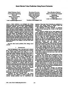
We sample 10% of the page views in order to conduct a preliminary data investigation. The average dwell time at each page depth is shown in Figure 2. For example, the maximum average dwell time is 15.42s at the page depth of 35%. According to this figure, the average page depthlevel dwell time becomes larger initially and then decreases on the second half of webpages. Users spend less time at the top and bottom areas of web pages. This is because the top areas typically contain the navigation bar, mostly titles in big font, or advertisements while the bottom areas contain mostly recommendation to other articles. Users tend to quickly skip these areas and go to the body of content. After reading the body of content, users often leave pages without reading the recommended links. Figure 3 shows the fraction of page depths whose dwell times are at least 1 second, which is the default duration threshold set by IAB. The threshold can be customized by publishers and especially advertisers. In our experiments (Section 5), we evaluate the proposed models under different duration thresholds. Figure 3 can be derived from Figure 2 by setting a dwell time threshold, i.e., 1s because the curves share a very similar shape. It can also be observed that page depth viewability has three phases: It goes up initially and gradually decreases once it reaches the page percentage of 20%. In the last quartile of a page, the viewability goes down at a larger rate.


Fig. 3: The Distribution of Page Views whose Dwell Times at the Corresponding Page Depths Are at Least 1s

4

Fig. 5: The Distribution of The Number of User Actions in a Page View

4 4.1

W EBPAGE D EPTH V IEWABILITY P REDICTION Problem Description

Problem Definition. Given an incoming page view (i.e., a user u and a webpage a) and the required minimum dwell time t, the goal is to predict the viewability of all page depths, denoted as v1 (u, a), ..., v100 (u, a), i.e., a page depth is viewable if its dwell time will be at least t seconds. The prediction is made after the page was requested by the user and before the user engages with the page. Fig. 4: The Cumulative Distribution of Page-Depth Dwell Time

Figure 4 shows the cumulative percentage of all pagedepths over increasing dwell time. We notice that 38.87% of all page depths have the dwell time of 0 seconds. This means that the users either quickly scroll past these page depths or leave the pages before scrolling to these page depths. This is intuitive in that users skip the uninteresting areas and only focus on the content they have interest. We also observe that the cumulative percentage for dwell time up to 60 seconds is 94.04%. In other words, users usually spend no more than one minute at one page depth. Since we use a real-life dataset, it is inevitable to observe outliers in which the depth-level dwell time is extremely high, e.g., hundreds of seconds. This is due to the fact that some users leave the web pages open and go away from their computers. These outliers have no value for the dwell time prediction. Thus, according to the results in Figure 4, we set a threshold of 60 seconds for depth-level dwell times. The entire page view is discarded from the dataset if the dwell time of one of its depth exceeds 60 seconds. Figure 5 shows the distribution of the number of user actions in a page view. A user action is defined as a reading event if a user scrolls to a part of a page and stays for at least one second. A majority of page views have few actions. For example, 26.96% of page views have only 1 action. There are 98.56% page views which have no more than 20 actions. The results make sense because most users do not engage much with pages. It is also observed that outlier page views with as many as 297 user actions exist in the dataset. Therefore, to remove the outliers, we discard the page views that have more than 20 user actions.

In addition, another goal is to predict the exact dwell time. The main difference is the output. The output for the first goal, which solves a classification problem, is a probability value in the interval [0,1]. The output for the second goal, which solves a prediction problem, is a non-negative value in the interval [0,+∞]. We develop and implement models to address both problems and show results in the Section 5. 4.2

Background of LSTM RNN

Before discussing the proposed solution, we would like to briefly introduce LSTM RNN first. A recurrent neural network (RNN) [18] is a type of artificial neural network whose connections form cycles, which enable RNN to handle long-term dependencies problems. Unlike feedforward neural networks, RNN can use their internal memory to process arbitrary sequences of inputs. However, traditional RNNs suffer from the vanishing or exploding gradient problem [19]: the network output either decays or blows up exponentially as it cycles around the network’s recurrent connections, due to the influence of a given input on the hidden layer. Specifically, in the case of decay, the gradient signal between time steps gets smaller so that learning either becomes very slow or stops. This makes the task of learning long-term dependencies in the data more difficult. In addition, if the leading eigenvalue of the weight matrix is more than 1.0, it can increase the gradient signal, so that it can cause learning to diverge. To avoid the long-term dependency problem, Long Short-term Memory (LSTM) networks [11] have been proposed. The LSTM network is a type of recurrent neural network used in deep learning because it can successfully train for very large architectures. The LSTM networks are good at handling the cases that contain many long sequences. The architecture of LSTM is designed to remember


information for long periods of time. The key to LSTMs is the multiplicative gates, which allow LSTM memory cells to store and access information over long periods of time, thereby avoiding the vanishing and exploding gradient problem. Gates are a way to optionally let information through. Researchers use a sigmoid neural net layer and a pointwise multiplication operation to implement gates. The output of the sigmoid neural net layer is either 0 or 1. A value of 0 means a blocked way and a value of 1 means an unobstructed way. The binary output of the sigmoid network describes how much of each component should be let through. LSTM RNNs have been shown to learn longterm dependencies more easily than the simple RNNs. The main advantage of LSTM RNN compared to Markov chains and hidden Markov models is that it does not consider the Markov assumption, and thus can be better at exploiting the potential patterns for modeling sequential data. Also, LSTM RNN can discover deep relationship between two time steps, as well as the input of a time step and the outcome. The sequential dependency between the dwell time of different depths is so complex and dynamic that time series analysis of Markov model approaches are not capable to model it effectively. Because of its good performance, LSTM RNN has been used in language modeling [20], speech recognition [21], and user searching behavior [22]. 4.3

The Proposed Models

We propose to use LSTM RNN to solve the webpage depth viewability prediction problem. In particular, we developed four models: 1) LSTM RNN; 2) LSTM RNN with embedding interaction; 3) bi-directional LSTM RNN with embedding interaction; 4) residual encoder-decoder (RED) bi-directional LSTM RNN with embedding interaction. 4.3.1 LSTM RNN Model Many factors can influence a user’s emotion and cognition when the user is reading a page. It is intuitive that the dwell time of a page depth is highly related to the user’s interests and reading habits [23], the topic of the article in the page, aesthetic design at that page depth, etc. Different users may have different reading patterns on an interesting page [17], [24]. Thus, the characteristics of individual users, webpages, and page depths should be taken into account for depthlevel dwell time prediction. However, it is non-trivial to explicitly model user interests, page characteristics, and the attractiveness of page depths. Web content publishers usually do not have detailed user profile information, including gender and age. The only user profile they may know is the user agent in the HTTP request and the user geo locations inferred from IP addresses. Also, modeling page interestingness and popularity is still an open research problem. More importantly, the complex interactions of these three factors must be modeled so that their joint effect is captured: 1) The interaction of users and pages captures a user’s interest in a page. 2) The interaction of users and page depths can reflect individual users’ browsing habits. For example, some users read entire pages carefully, but some only read the upper half. 3) The interaction of pages and depths models the design of individual pages at individual page depths.

5

For example, pages that have a picture at a depth may receive relatively short dwell time at that depth because people usually can understand a picture quicker than text. Therefore, predicting user reading behavior at page depth level is highly challenging. The work in [6] is the most related to this study; it applies Factorization Machines (FM) to predict the webpage depthlevel dwell time. However, the existing solution has two limitations: 1) The latent features learnt by matrix factorization cannot discover the deep joint effect of the input variables. The FM model learns latent features for input variables through a one-layer shallow network. It has limited ability to discover and utilize deep relationship between the input and the outcome. 2) The user engagement with the previous page depth in the same page view is not considered. For instance, if a user is predicted to spend long time at the page depths from 1% to 20%, the user probably will stay long at the page depth 21% as well. This LSTM RNN model addresses these limitations as follows: (1) It uses a deep neural network to capture the underlying patterns between many input factors and webpage depth viewability. (2) The proposed deep learning model takes into account the predicted viewability of the previous page depths in the same page view. Our LSTM RNN considers the webpage depth-level viewability prediction as a sequential prediction problem, in which the predictions at the time steps (i.e., page depths) can influence the prediction at the current time step. We use LSTM in conjunction with RNN because the length of each sequence in our application is as long as 100 and a traditional RNN will suffer from the vanishing or exploding gradient problem.

Fig. 6: Modelling Webpage Depth Viewability Prediction Figure 6 presents the method used to solve the ’manyto-many’ prediction problem by our LSTM RNN. The left side is a webpage, which has 100 page depths. Each page depth corresponds to one time step in the RNN setting, as shown in the right side of the figure. The proposed method makes predictions at every time step. The prediction is the


6

a user u at depth d in a sequence, rud denotes the representation of the depth d’s input of a user u. f (x) is the activation function, and the b terms (i.e., bh and by ) are bias vectors. C ∈ Rn×n and W ∈ Rn×n are the transition matrix for current depths and the previous status, respectively, where n is the dimension of the embedding vector. W can propagate sequential signals, and C can capture users’ current behavior. With the suggestions of the domain experts at Forbes, we consider significant information in the input layer. In particular, the input layer concatenates several components: •

•

Fig. 7: The LSTM RNN Model viewability of the page depth in the specific page view. The input of each time step includes information about the user, the page, the depth, and the context. Since the LSTM layers of each time step can generate a viewability prediction, the hidden neurons in the LSTM should carry information about the viewability of that time step. The hidden layers at page depth i should be able to summarize the viewabilities from page depth 1% to i. Therefore, using LSTM to pass the information of the previous time steps can incorporate the previously-predicted viewability into the prediction at the current time step. Note that, since the prediction for a page view is made before page loading, the true viewability of all page depths are unknown. Thus, the predicted viewability of the past page depths are used to predict that of the current depth. The outputs at all page depths v1 (u, a), ..., v100 (u, a) are counted to compute the performance. Thus, the problem is modeled as a sequence labelling (e.g. Part-of-speech tagging), where the true labels of the past are unknown, instead of time-series (e.g. stock price prediction), where the true labels of the past are used in prediction. Figure 7 presents the architecture of the proposed (rolling) LSTM RNN used in webpage depth viewability prediction. At each page depth, the LSTM RNN consists of one input layer, two LSTM hidden layers, one output layer, and the inner weight matrix. Given a user input sequence x = (xu1 , . . . , xut ), the hidden layers vector sequence h = (hu1 , . . . , hut ) and the output vector sequence y = (y1 , . . . , yt ) are computed by iterating the following equations from the page depth d = 1 to t

hud = f (Whud−1 + Crud + bh )

(1)

yd = f (Whud + by )

(2)

Where hud ∈ R2 denotes the hidden representation of

•

•

•

•

•

The user’s viewport size, i.e., viewport height and width. A viewport is the part of a user browser visible on the screen. The viewport indicates the device utilized by the user (e.g., a mobile device usually has a much smaller viewport) and can directly determine the user experience. To reduce sparsity, both heights and widths are put into buckets with size 100 pixels. The user’s geo location, which is detected from user IP addresses. Since individual users are identified by cookie IDs, it is possible that the same user visits the website from different locations in multiple sessions. We consider user geo locations because this is the only explicit feature about users that can be easily obtained by publishers without violation of user privacy. In practice, user geo may reflect a user’s interests and education. Specifically, geo is the country name if the user is outside USA or a state name if she is within USA. local hour, and local day of the week (denoted by weekday in the experiments), which are likely related to user reading behavior. Article length is represented by the word count of the article in the page, and it has been proven to be a significant factor impacting page-level dwell time [13]. Here, we utilize this feature because it allows us to model the user effort in consuming the content up to a given scroll depth. Article lengths are put into buckets, so that there are a limited number of possible states. Freshness is the duration between the reading time and the time the page was published on the website. Freshness is measured in days. The freshness of an article may determine the interests of a user on it. Fresh news may receive more user engagement. The channel and section of the article in a page are its topical categories on the publisher’s website, e.g., finance and lifestyle. A channel can be considered as a high-level topic label of a page. A section is defined as a sub-channel at finer topical granularity. Other page attributes in the Forbes article metadata are also taken into account: page type (e.g., “blog”, “blogslide”, or “trendingactivity”), whether the page is in standard template type, whether the page contains any image, whether the article is written by Forbes staff, and the number of user comments. All context variables are modeled by one-hot encoding for simplicity. As one common step of feature engineering, rarely-occurred feature values are grouped into “ OTHER” categories.


Existing studies [22], [25] use mostly one-hot encoding to represent the categorical variables which have millions of values. However, this encoding increases a lot the sparsity and width of the input layers. More importantly, it learns a very limited representation of the variables. Therefore, it is important to use a rich and dense representation to model the most important categorical variables in the data. To this end, our LSTM RNN uses three embedding layers to model the three most important categorical variables: user, page, page depth. Before concatenating and feeding the four components to the LSTM layers, we apply dropout to each component. Dropout [26] is a simple and effective method to prevent a neural network from overfitting. In particular, it randomly sets a fraction of the units in an output vector to 0 at each update during training time. By cross validation, the fraction is set to 20%. Stacked above the input layers are multiple LSTM layers. The number of layers is a parameter that can be tuned by experiments. Each can be considered as one reasoning step based on the output of the previous layer. The number of hidden nodes in each LSTM can be empirically determined. Each LSTM layer has two outputs: 1) The first output carries the information of this time step and is sent to the counterpart at the next time step through a complex set of gates. 2) The second output is passed to the next layer by an activation function. Specifically, the activation function we use is the Tanh function (Equation 3), which is non-linear and outputs values in the (-1,1) range.

2 −1 (3) 1 + e−2x Unlike the sigmoid function whose output is not zerocentered, the Tanh function is less likely to get the network stuck in the current state during training. Also, the Tanh function is not as fragile as the Rectified Linear Unit (ReLU). A large gradient flowing through a ReLU neuron could cause the weights to update in such a way that the neuron will never activate on any data point again. We also apply dropout to the output of each LSTM layer: 20% units in the output are randomly picked and set to 0. The vertical output of the last LSTM x are passed into a sigmoid function (Equation 4), which outputs a value that in the [0,1] range. tanh(x) =

1 (4) 1 + e−x The output represents the page depth viewability, i.e., the probability that the page depth will be viewable. sigmoid(x) =

4.3.2 LSTM RNN with Embedding Interactions Model The model presented so far (termed LSTM noInteract from now on) can be further improved by capturing the interactions of the three important factors: user, page, and page depth. The extended model introduced in this section is denoted as LSTM Interact. Like most of general neural networks, the LSTM noInteract only captures the OR relationships among input factors, rather than the AND relationship. The input of an activation function at a layer is a linear combination of the input units passed from the previous layer. For

7

Fig. 8: Example of Propagation without Interaction

Fig. 9: Example of Propagation with Interaction

instance, Figure 8 shows a part of an example network. The two embedding vectors have values [p1 , p2 , ..., pn ] and [q1 , q2 , ..., qn ], respectively. n is the length of the embedding layers. The input of the neuron yj in the next layer is shown in Equation 5 (assuming the activation function is p tanh). wi,j is the weight in connecting the ith neuron in q the embedding 1 to the neuron yj . wi,j is the weight in connecting the ith neuron in the embedding 2 to the neuron yj . pi and qi are the values of the ith neuron in embedding 1 and 2, respectively. n is the length of the latent vectors. Thus, like all vanilla neural networks, the LSTM noInteract does not consider the pairwise interaction of the embedding layers. n n X X p q yi = tanh( wi,j × pi + wi,j × qi ) i=1

(5)

i=1

To solve this problem, we use knowledge from the recommender system field. For example, to predict a movie rating for an unseen user and movie pair, one simple way is to use matrix factorization, e.g., Singular Vector Decomposition (SVD). SVD learns a latent vector for each user/item. Given an unseen user and item pair, the dot product, i.e., the interaction, of the user latent vector pu and the page latent vector qi is the predicted outcome, e.g., a movie rating: rûi = qiT pu . In other words, it sums up all values generated by element-wise vector multiplication (i.e., multiplying two embedding vectors element by element). In our case, the embedding vector of an entity can be regarded as a latent vector in SVD. Thus, we can use a similar method to capture the interaction of multiple input factors. Figure 9 is an example for the interaction between user and page. The embedding layers learn user embedding and page embedding with same dimension. Then, the model generates the interaction layer based on element-wise vector multiplication between the user embedding and the


8

page embedding. We use the same method to capture the interaction between user and page depth, as well as page and page depth. Assuming the activation function is tanh, an element yi in the interaction vector is defined as:

yi = tanh(pi ∗ qi )

(6)

For example, the interaction of [1 0 3] and [2 3 7] is [2 0 21]. The interaction of two embedding layers of length d is a vector of length d. The resulting values will be summed up with other factors in the next layer.

Fig. 10: The LSTM RNN with Embedding Interaction Model

Fig. 11: The Bi-directional LSTM RNN with Embedding Interaction

Therefore, at the input layer of the second model, we also consider the 2-way interaction and the 3-way interaction of user, page, and depth embeddings (shown in Figure 10). The resulting four interaction vectors are then concatenated with the other input vectors that are already considered in the LSTM noInteract. This extended model is denoted as LSTM Interact. 4.3.3 Bi-directional LSTM RNN Model It is commonly-observed that users often scroll-back on pages as well. Therefore, dwell time of lower page depths could indicate the dwell time of upper page depths. For instance, a user who spent a long time at the last paragraph of an article and is scrolling up will probably stay long in the middle of the page. The possible reason is that the last paragraph may rekindle the user’s interest to the entire article. In this case, single directional LSTMs fail to capture such backward patterns to improve prediction performance. Moreover, in single directional LSTM, predictions made at very top page depths rely on few previous page depths. For instance, as the Figure 6 indicates, only the LSTM layers at the page depth of 1% can contribute to the prediction at the page depth of 2%. Only the LSTM layers of 1% is known when predicting the output of 2% because predictions are made sequentially from page top to the bottom, i.e. single direction. The information of the page depths after 2% are inaccessible. In this case, relying on very few previous information can lead to unreliable prediction outcome at

Fig. 12: Bidirectional LSTM Recurrent Neural Network (from [21])

very top page depths. Less accurate prediction at top page depths may distort the predictions at further page depths. Such problem can be overcome if the page depths after a current one can be taken into account. In this case, the prediction at any page depth considers the information of the other 99 page depths. Therefore, it may be helpful to enhance the proposed models using a bi-directional LSTM RNN [21], which propagates information in both directions. As Figure 12 shows, Bi-


9

directional LSTMs combine a single directional LSTM that moves forward through time, beginning from the start of a sequence, with another LSTM that moves backward through time, beginning from the end of a sequence. It allows the output at a time step t to compute a representation that depends on both the past and the future but in most sensitive to the input around the input at t, without having to specify a fixed-size window around t [27]. A bi-directional LSTM RNN iterates the backward hidden layer from d = t to 1, and the forward layer from d = 1 to t. Then it can − → compute the forward hidden sequence h , the backward ← − hidden sequence h and the output sequence y as follows

− → − → − → − → hud = f (W hud−1 + C rdu + b h )

(7)

← − ← − ← − ← − hud = f (W hud−1 + C rdu + b h )

(8)

− → ← − yd = f (W hud + W hud + by )

(9)

Fig. 13: RED-BLSTM˙Interact Structure

In particular of our case, the bi-directional LSTMs replace the LSTM layers in Figure 10: one forward LSTM and one backward LSTM running in reverse direction and with their outputs merged at the output layer. Figure 11 shows the architecture of the proposed bi-directional LSTM RNN. The forward LSTM operates as usual: it carries information of the past page depths. In contrast, the backward LSTM flows from the page bottom to the top. It brings information about the dwell time of the page depths that are lower than the current page depth. Along with the input at the current page depth, their outputs are then merged by element-wise averaging because they would equally contribute to the outcome of the page depth. A dropout of 20% follows to avoid overfitting. In this way, bi-directional LSTMs enable information from both past and future to come together. Bi-directional LSTM RNNs have been used in speech recognition [21] and bio-informatics [28]. Bi-directional LSTMs are useful in some applications, where the prediction outcome of a time step depends on the entire input sequence, rather than only the past and present. To the best of our knowledge, we are the first to apply bi-directional LSTM networks in user behavior prediction. This bi-directional LSTM RNN is denoted as BLSTM Interact. 4.3.4 Residual Encoder-Decoder Bi-directional LSTM RNN Model One limitation to training stacked LSTM layers is the vanishing gradient problem. Adding residual connections between LSTM layers has been shown effective in a recent Google’s Neural Machine Translation study [9]. Inspired by this work, we add residual connections between our bi-directional LSTM layers, as shown in Figure 13. Residual connections add a “highway” to skip some layers. Instead of hoping each few stacked layers directly fit a desired underlying mapping, residual networks explicitly let these layers fit a residual mapping [29], [30]. The idea of residual connection can be formally expressed as:

xl = Hl (xl−1 ) + xl−1

where xl−1 and xl are the input and output of the lth units, and Hl (.) denotes the residual function.

(10)

For the residual function Hl (.), we consider sequenceto-sequence LSTM embedding, which comprises of two bidirectional LSTM layers; one is used for encoding, and the other for decoding. The difference between the encoder and the decoder is the output dimensionality, i.e., number of neurons in each layer. The BLSTM encoder has much smaller dimensionality than the decoder. The ouput dimentionality of the deconder is the same with the input of encoder. Sequence-to-sequence LSTM embedding is effective to improve classification accuracy through learning feature representation and removing noise [31]. The idea originated in autoencoder, an artificial neural network for efficient coding that is widely used in sematic learning and feature reduction [32], [33]. It has two phases: an encoder phase h(·) maps an input layer x ⊂ Rn to the hidden layer h(x) ⊂ Rk , and a decoder phase g(·) maps the hidden representation h(x) back to the original input space g(h(x)) ⊂ Rn . The parameters of autoencoders are learned from minimizing the difference between the input and the output, i.e., loss L(x, g(h(x)). The dimension of the learned embedding is k , which is typically much smaller than its original dimensionality n. The difference between our encoder-decoder structure and autoencoder is that an autoencoder learns feature representation or reduction as in unsupervised learning problems. Our model, on the other hand, directly utilizes the reconstructed features g(h(x)) instead of the embedding layer h(x). Compared with the original input data x, it can remove noise in the reconstructed data g(h(x)). Another benefit is that it can reduce the computational cost by using a smaller number of neurons in the decoder BLSTM layer.

5 5.1

E XPERIMENTAL E VALUATION Settings

A three-week user log is collected from a real business platform as described in Section 3. The user log contains user visits of Forbes article pages. After pre-processing, the final dataset contains about 40K unique users and 30K unique pages. The dataset is split into training, validation and test data sets. To build training data, some existing studies [6] iteratively set a threshold and select only frequent users and


pages/items in the training data. However, in this work, following the suggestion of [34], our training data contains all users and pages, including casual users and niche pages. The reasons are 1) deep learning models require large input dataset in order to avoid overfitting; 2) the model can handle more users an pages which do not occur frequently. 3) in practice, new pageviews with unseen users or pages can be directly used to incrementally train the models with stochastic gradient descent. To build validation and test data, we randomly select pageviews whose users and pages occur at least five times in the training data. These pageviews are exclusively separated into the validation and test sets. In this way, we avoid coldstart problem: all users and pages in the validation and test sets occur at least five times in the training data. As a result, the training set, validation set, and test set contain about 100K, 11K, and 11K pageviews, respectively. One page view has 100 page depths, i.e., time steps. Since the RNN LSTM parameters are shared by all time steps, the parameters are trained based on about 10M page depths in each epoch. At the beginning of each epoch, the training data is shuffled. The error on the validation set is used as a proxy for the generalization error. We use validation-based early stopping to obtain the models that work the best with the validation data. Since it is common that the validation error may fluctuate during training (producing multiple local minima), the maximum number of epochs is set to 10. By observing the curve of validation errors, it can be guaranteed that overfitting occurs within the first 30 epochs. The models with the minimum validation error are saved and used to predict the testing data. We observe that the minimum validation errors are often obtained at the 4th-6th epochs. In addition, since the exact prediction performance varies by several factors, e.g., parameter initialization, all models are run three times. The reported performance results are obtained by averaging the three runs. 5.2

Implementation

The proposed LSTM RNN models are implemented using Keras [35] with Theano [36] backend. The experiments are run on a desktop with i7 3.60Hz CPU and 32GB RAM. The matrix computation is sped up using NVIDA GeForce GTX 1060 6G GPU. Running 10 epochs usually takes 5-8 hours depends on the parameter setting. Considering the training speed and memory consumption, we set the training batch size to 256. Existing work [37] indicates that a large batch size might alleviate the impact of noisy data, while a small one sometimes can accelerate the convergence. Hence, we varied the batch size, e.g., 128 and 512, but no significant differences have been observed. During the training processes, the parameter is initialized by sampling from a uniform distribution. The optimizer we adopt is Stochastic Gradient Descent (SGD), which can can overcome the high cost of backpropagation and still lead to fast convergence, with a learning rate of 0.01, a learning rate decay of 1e-6, and a momentum of 0.99. Nesterov momentum is also enabled. An existing study [38] finds that momentum-accelerated SGD are effective for training RNNs. We also tried RMSprop and Adam optimizers. Al-

10

though Adam can further accelerate convergence, neither beats SGD for the performance.

5.3

Comparison Models

GlobalAverage: In a training page view, if the dwell time of a page depth is at least t seconds, the viewability of the page depth in the page view is considered to be 1; otherwise, it is 0. Therefore, we can calculate what percentage of page views are viewable at each page depth. The 100 constant numbers obtained are used to make deterministic predictions for the corresponding test page depths. Logistic Regression (LR): Since the viewability prediction can be considered as a classification problem. A logistic regression model is developed as a baseline. The input variables are almost the same as those used in the proposed model. LR models user, page, and depth using one-hot encoding. Using Keras, we develop a one-layer neural network with sigmoid activation function to mimic a logistic regression. The LR is trained following the same process as the proposed models. The learning method is also SGD with learning rate 0.001. Factorization Machines (FM): Factorization machines (FM) [16] are a generic approach that combines the highprediction accuracy of factorization models with the flexibility of feature engineering. This method has been widely used in many applications. The basic idea of FM is to model each target variable as a linear combination of interactions between input variables. Formally, it is defined as following.

yˆ(x) = w0 +

n X i=1

w i xi +

n−1 X

n X

hvi , vj i xi xj

i=1 j=i+1

where, yˆ(x) is the prediction outcome given an input x. w0 is aPglobal bias, i.e., the overall average depth-level dwell n time. i=1 wi xi is the bias of individual input variables. For example, some users would like to read more carefully than others; some pages can attract users to spend more time on them; some page depths, e.g., very bottom of a page, usually receive little dwell time. The first two terms are the same as in linear regression. The third term captures the sparse interaction between each pair of input variables. In the experiments, the FM model is implemented based on [6]. The proposed FM model considers four input variables: user, page, depth, and viewport size.

5.4

Metrics

As mentioned in Section 4.1, there are two ways to handle dwell time prediction: one computes the probability that a given page depth is shown on the user screen for a given dwell time (i.e., a classification problem); the other predicts the exact dwell time at each page depth. To measure the classification performance, we adopt Logistic Loss, Accuracy, Area Under Curve (AUC). To evaluate the exact dwell time prediction, we adopt RMSD. Logistic Loss: It is widely used in probabilistic classification. It penalizes a method more for being both confident and wrong. Lower values are better.


logloss = N 100

−

XX 1 [yij log(ˆ yij ) + (1 − yij ) log(1 − yîj )] N · 100 i=1 j=1

where N is the number of the test page views. Each has 100 page depths, i.e., 100 prediction outputs. yîj is the predicted viewability and yij is the actual viewability at the j th page depth in the ith page view. Area Under Curve (AUC): The AUC is a common evaluation metric for binary classification problems, which is the area under a receiver operating characteristic (ROC) curve. An ROC curve is a graphical plot that illustrates the performance of a binary classifier system, as its discrimination threshold is varied. The curve is created by plotting the true positive rate against the false positive rate at various threshold settings. If the classifier is good, the true positive rate will increase quickly and the area under the curve will be close to 1. Higher values are better. Accuracy: The accuracy classification score computes the percentage of the test instances which are correctly predicted. It is noticed that the accuracy scores may be slightly influenced by the threshold. We choose accuracy as an intuitive metric and set the threshold to the ordinary setting value of 0.5 [39], [40] in our experiment. Compared with accuracy, AUC and Logistic Loss are not influenced by specific thresholds. They are better metrics if the class distribution is highly imbalanced. Root-mean-square Deviation (RMSD): It is used in dwell time prediction, which is a regression problem. RMSD measures the differences between the values predicted, yî , and the values observed, yi . s PN P100 yij − yij )2 j=1 i=1 (ˆ RM SD = N · 100

N is the number of test page views. The second sum accumulates the errors at all 100 page depths in the ith page view. yij is the actual dwell time at the j th page depth in the ith page view. Lower values are better. 5.5

Comparison of Our Proposed Models

11

data. The models contains two LSTM layers, each of which has 500 hidden neurons. The embedding layers have 500 hidden neurons. This network configuration is obtained experimentally, as discussed in Section 5.7. To evaluate the models’ performance with different viewability thresholds, i.e., minimum required dwell time, we set three thresholds: 1s, 5s, and 10s. The viewability threshold of 1s is in line with the viewability definition suggested by the IAB. In the experiment, the models are compared by log-loss, accuracy and AUC. However, since we observed that the model with lower log-loss also has higher accuracy and AUC, only the log-loss results are shown. The RED-BLSTM Interact model performs best, as it leverages residual connections and encoder-decoder structure for better learning. The results verify that the residual encoder-decoder method can consistently enhance the performance for all metrics under all three viewability thresholds. We also notice that the effectiveness of BLSTM Interact in utilizing the predicted behavior for both past page depths and future page depths. In addition, LSTM Interact performs better than LSTM noInteract because it captures the embedding interaction. Comparing across viewability thresholds, the performance for 1s is the best. Surprisingly, the performance for 5s is not as high as that of 10s. This is because the number of positive instances, i.e., the page depths whose dwell times are at least 5s, and negative instances, i.e., the page depths whose dwell times are less than 5s are almost equal (as shown in Figure 4). This makes the prediction more challenging. 5.6

Performance Comparison with Other Baselines

This section compares our two best model, REDBLSTM Interact and BLSTM Interact, with other comparison methods using the log-loss, accuracy, and AUC metrics. The parameter settings of the proposed model is the same as the ones used previously. Tables 2, 3, and 4 present the performance comparison with three viewability thresholds. The RED-BLSTM Interact and RED-BLSTM Interact models are clearly better than the comparison methods for all three metrics: The lower logloss indicates that our models have fewer mistakes due to over-confidence, and this is also reflected in the accuracy results. The higher AUC values show that our models also obtain better performance on average by varying the decision boundary from 0 to 1. The results verify that our sequential neural network models can consistently enhance the performance for all metrics under all three viewability thresholds. TABLE 2: Viewability Prediction. Threshold = 1s

Fig. 14: Log-loss Performance of Our Models This section compares the performance of the proposed models. Figure 14 shows their performance in the test

Approaches GlobalAverage Logistic Regression FM BLSTM Interact RED-BLSTM Interact

Logloss 0.6586 0.6484 0.6273 0.6016 0.5985

Accuracy 59.45% 63.36% 64.88% 67.36 % 67.70%

AUC 61.98% 62.55% 66.11% 71.54 % 71.97%

The performance of our models, and especially of REDBLSTM Interact, is significantly better than that of FM.


12

TABLE 3: Viewability Prediction. Threshold = 5s Approaches GlobalAverage Logistic Regression FM BLSTM Interact RED-BLSTM Interact

Logloss 0.6786 0.6726 0.6527 0.6250 0.6226

Accuracy 57.35% 58.94% 60.13% 64.87% 65.28%

AUC 59.42% 61.47% 63.54% 70.72% 71.24%

TABLE 4: Viewability Prediction. Threshold = 10s Approaches GlobalAverage Logistic Regression FM BLSTM Interact RED-BLSTM Interact

Logloss 0.6635 0.6546 0.6332 0.6076 0.6049

Accuracy 59.65% 60.40% 62.58% 66.98% 67.37%

AUC 58.46% 61.61% 63.96% 70.94% 71.37%

This shows that a deep neural network can discover more underlying patterns between input variables, which can then improve the overall performance. The dependency between page depths also contributes to better viewability prediction. The Logistic Regression uses one-hot encoding to represent the user, page, and page depths. Thus, it has limited capability to fit the data as well as the FM which builds latent vectors to model the three categorical variables. The GlobalAverage always makes the deterministic prediction using the fraction of positive page depths computed based on the training data. Its performance is the lowest compared with the other methods. 5.7

Effect of Main Parameters

In this section, we tune the model by varying some important parameters: the sizes of the embedding layers, and the number of LSTM layers. In these experiments, the minimum dwell time threshold is set to 5s, in which case the number of negative training instances is almost the same as the number of positive training cases. Note that the same experiments have been conducted for the other two proposed models, but due space constraints we show results only for BLSTM Interact and RED-BLSTM Interact, which achieve the best performance. Figure 15a shows the effect of the dimensionality of the embedding layers, i.e., the number of hidden neurons in an embedding layer. It contains two LSTM layers and the metrics are computed over the test data. To simplify the solution space, we apply the same dimensionality for user embedding, page embedding, and depth embedding. Varying the dimensionality of the embedding layers also change the dimensionality of the interactions. When varying the embedding layer sizes, we fix the dimentionalities of the bi-directional LSTM layers to 500. The results show that higher-dimensional word embeddings do not always provide better performance. This finding is in line with existing work [41] that applies word embeddings in a Name Entity Recognition task. Although intuitively wider embedding layers should have finer representation, they also tends to cause overfitting. On the other hand, too narrow embedding layers cannot capture well the traits of input variables. Embedding=500 obtains

the lowest log-loss in the test data. It also has the highest accuracy. However, Embedding=600 is slightly better than Embedding=500 for the AUC score. This implies that Embedding=500 is better than Embedding=600 for the decision threshold of 0.5. But when considering all thresholds on average, Embedding=600 is slightly better. On the other hand, narrower embedding layers have fewer parameters to learn, which requires less training data and shorter training time. Therefore, Embedding=500 may still be preferable in practice. Figure 15b presents the effect of the numbers of the bi-directional LSTM layers stacked sequentially. Each bidirectional LSTM layer has 500 hidden neurons in each direction. It clearly illustrates that the performance can be significantly improved by increasing the number of bidirectional LSTMs from 1 to 2. But all three performance curves become flat for 3 layers and worse after adding the fourth layer. Figure 15c presents the effect of the number of BLSTM layers in RED-BLSTM Interact model. The decoder BLSTM has 500 hidden neurons and the encoder BLSTM has 100 hidden neurons in each direction. The results show the performance gets worse with the increase of residual encoderdecoder layers. This finding is different from that obtained for residual neural networks for image processing [29]. The reason is that the input of images has typically a much higher dimensionality. In our problem, we need a wider deep network to learn a richer representation of the input entity. A hidden layer with more hidden nodes can capture more latent features of a user, a page, a depth, or their interaction with the context. Also, it is necessary to capture more latent aspects of individual user, page, and depth without explicit features. In addition, Figure 15b shows that two LSTM layers are enough to fit well the user behavior data. Although user behavior is difficult to learn, the user behavior prediction problem usually does not require too many reasoning steps vertically at each time step [22], compared with the deep networks used in computer vision [42]. 5.8

Performance of Exact Dwell Time Prediction

The proposed models for page depth viewability prediction can also be applied to predict the exact dwell time of a page depth. This can also be useful for publishers and advertisers: For example, predicted depth-level dwell time can help publishers quantify the interestingness of a page depth to a specific user. In this case, the publisher can determine at which depth is preferable to show recommended article links. Also, advertisers may want to know the exact dwell time that a user will spend at a page depth. As mentioned in section 4.1, the main difference between viewability prediction and exact dwell time prediction is the output. Thus, in order to make page depth dwell time prediction, we change the activation function of the output layer from a sigmoid function to a rectified linear unit (ReLU). Given a input x of a linear combination sent from the previous layer, ReLU converts it by Equation 11 .

relu(x) = max(0, x)

(11)

Thus, the output of a ReLU is a non-negative value. In addition, the learning rate is reduced from 0.01 to 0.001


(a) Varying the Embedding Widths

13

(b) LSTM layers in BLSTM Interact

(c) LSTM layers in RED-BLSTM Interact

Fig. 15: Effect of Main Parameters

R EFERENCES [1] [2] [3]

[4]

Fig. 16: Performance of Dwell Time Prediction

[5]

[6]

because 0.01 is too large for the regression problem. We use the mean squared deviation as the objective function. The results are calculated based on all test page depths. Figure 16 shows that the proposed deep learning models significantly outperform the comparison systems. The REDBLSTM Interact generates the least RMSD.

[7]

6

[9]

C ONCLUSIONS

Online publishers and advertisers are interested to predict how likely it is that a user will stay at a page depth for at least a certain dwell time, defined as webpage depth viewability. Viewability prediction can maximize publishers’ ad revenue and boost advertisers’ return on investment. This paper presented four deep sequential neural networks based on Recurrent Neural Network (RNN) with the Long Short-Term Memory (LSTM). The proposed models predict the viewability and exact dwell time for any page depth in a specific page view. Using a real-world dataset, the experiments consistently show our models outperforming the comparison models.

ACKNOWLEDGEMENT This work is partially supported by NSF under grants No. CAREER IIS-1322406, CNS 1409523, and DGE 1565478, by a Google Research Award, and by an endowment from the Leir Charitable Foundations. Any opinions, findings, and conclusions expressed in this material are those of the authors and do not necessarily reflect the views of the funding agencies.

[8]

[10] [11] [12]

[13] [14]

[15]

[16] [17]

Google, “The importance of being seen,” https://think.storage.googleapis.com/docs/the-importanceof-being-seen study.pdf,2014. C. Wang, A. Kalra, C. Borcea, and Y. Chen, “Revenue-optimized webpage recommendation,” in 2015 IEEE International Conference on Data Mining Workshop (ICDMW). IEEE, 2015, pp. 1558–1559. P. Yin, P. Luo, W.-C. Lee, and M. Wang, “Silence is also evidence: interpreting dwell time for recommendation from psychological perspective,” in Proceedings of the 19th ACM SIGKDD international conference on Knowledge discovery and data mining. ACM, 2013, pp. 989–997. C. Wang, A. Kalra, C. Borcea, and Y. Chen, “Viewability prediction for online display ads,” in Proceedings of the 24th ACM International Conference on Information and Knowledge Management. ACM, 2015, pp. 413–422. C. Wang, A. Kalra, L. Zhou, C. Borcea, and Y. Chen, “Probabilistic models for ad viewability prediction on the web,” IEEE Transactions on Knowledge and Data Engineering, vol. PP, no. 99, pp. 1–1, 2017. C. Wang, A. Kalra, C. Borcea, and Y. Chen, “Webpage depth-level dwell time prediction,” in Proceedings of the 25th ACM International Conference on Information and Knowledge Management. ACM, 2016, pp. 1937–1940. Y. LeCun, Y. Bengio, and G. Hinton, “Deep learning,” nature, vol. 521, no. 7553, p. 436, 2015. A. Esteva, B. Kuprel, R. A. Novoa, J. Ko, S. M. Swetter, H. M. Blau, and S. Thrun, “Dermatologist-level classification of skin cancer with deep neural networks,” Nature, vol. 542, no. 7639, p. 115, 2017. Y. Wu, M. Schuster, Z. Chen, Q. V. Le, M. Norouzi, W. Macherey, M. Krikun, Y. Cao, Q. Gao, K. Macherey et al., “Google’s neural machine translation system: Bridging the gap between human and machine translation,” arXiv preprint arXiv:1609.08144, 2016. J. Schmidhuber, “Deep learning in neural networks: An overview,” Neural networks, vol. 61, pp. 85–117, 2015. A. Graves, “Supervised sequence labelling,” in Supervised Sequence Labelling with Recurrent Neural Networks. Springer, 2012, pp. 5–13. C. Liu, R. W. White, and S. Dumais, “Understanding web browsing behaviors through weibull analysis of dwell time,” in Proceedings of the 33rd international ACM SIGIR conference on Research and development in information retrieval. ACM, 2010, pp. 379–386. X. Yi, L. Hong, E. Zhong, N. N. Liu, and S. Rajan, “Beyond clicks: dwell time for personalization,” in Proceedings of the 8th ACM Conference on Recommender systems. ACM, 2014, pp. 113–120. Y. Kim, A. Hassan, R. W. White, and I. Zitouni, “Modeling dwell time to predict click-level satisfaction,” in Proceedings of the 7th ACM international conference on Web search and data mining. ACM, 2014, pp. 193–202. S. Xu, H. Jiang, and F. Lau, “Mining user dwell time for personalized web search re-ranking,” in Proceedings of the Twenty-Second International Joint Conference on Artificial Intelligence, vol. 22, no. 3, 2011, pp. 2367–2372. S. Rendle, “Factorization machines with libfm,” ACM Transactions on Intelligent Systems and Technology (TIST), vol. 3, no. 3, p. 57, 2012. D. Lagun and M. Lalmas, “Understanding user attention and engagement in online news reading,” in Proceedings of the Ninth ACM International Conference on Web Search and Data Mining. ACM, 2016, pp. 113–122.


[18] S. Lawrence, C. L. Giles, and S. Fong, “Natural language grammatical inference with recurrent neural networks,” IEEE Transactions on Knowledge and Data Engineering, vol. 12, no. 1, pp. 126–140, 2000. [19] R. Pascanu, T. Mikolov, and Y. Bengio, “On the difficulty of training recurrent neural networks,” in Proceedings of The 30th International Conference on Machine Learning, 2013, pp. 1310–1318. ¨ [20] M. Sundermeyer, H. Ney, and R. Schluter, “From feedforward to recurrent lstm neural networks for language modeling,” IEEE/ACM Transactions on Audio, Speech and Language Processing (TASLP), vol. 23, no. 3, pp. 517–529, 2015. [21] A. Graves, N. Jaitly, and A.-r. Mohamed, “Hybrid speech recognition with deep bidirectional lstm,” in 2013 IEEE Workshop on Automatic Speech Recognition and Understanding (ASRU), 2016. [22] A. Borisov, I. Markov, M. de Rijke, and P. Serdyukov, “A neural click model for web search,” in Proceedings of the 25th International Conference on World Wide Web. International World Wide Web Conferences Steering Committee, 2016, pp. 531–541. [23] M. Claypool, P. Le, M. Wased, and D. Brown, “Implicit interest indicators,” in Proceedings of the 6th international conference on Intelligent user interfaces. ACM, 2001, pp. 33–40. [24] M. Chen and Y. U. Ryu, “Facilitating effective user navigation through website structure improvement,” IEEE Transactions on Knowledge and Data Engineering, vol. 25, no. 3, pp. 571–588, 2013. [25] Y. Zhang, H. Dai, C. Xu, J. Feng, T. Wang, J. Bian, B. Wang, and T.-Y. Liu, “Sequential click prediction for sponsored search with recurrent neural networks,” in Twenty-Eighth AAAI Conference on Artificial Intelligence, 2014. [26] N. Srivastava, G. E. Hinton, A. Krizhevsky, I. Sutskever, and R. Salakhutdinov, “Dropout: a simple way to prevent neural networks from overfitting.” Journal of Machine Learning Research, vol. 15, no. 1, pp. 1929–1958, 2014. [27] Y. Bengio, I. J. Goodfellow, and A. Courville, “Deep learning,” An MIT Press book in preparation. Draft chapters available at http://www. iro. umontreal. ca/ bengioy/dlbook, 2015. [28] J. Hanson, Y. Yang, K. Paliwal, and Y. Zhou, “Improving protein disorder prediction by deep bidirectional long short-term memory recurrent neural networks,” Bioinformatics, p. btw678, 2016. [29] K. He, X. Zhang, S. Ren, and J. Sun, “Deep residual learning for image recognition,” in Proceedings of the IEEE conference on computer vision and pattern recognition, 2016, pp. 770–778. [30] L. Yu, X. Yang, H. Chen, J. Qin, and P.-A. Heng, “Volumetric convnets with mixed residual connections for automated prostate segmentation from 3d mr images.” in AAAI, 2017, pp. 66–72. [31] N. Srivastava, E. Mansimov, and R. Salakhudinov, “Unsupervised learning of video representations using lstms,” in International conference on machine learning, 2015, pp. 843–852. [32] Y. Bengio et al., “Learning deep architectures for ai,” Foundations R in Machine Learning, vol. 2, no. 1, pp. 1–127, 2009. and trends [33] P. Vincent, H. Larochelle, Y. Bengio, and P.-A. Manzagol, “Extracting and composing robust features with denoising autoencoders,” in Proceedings of the 25th international conference on Machine learning. ACM, 2008, pp. 1096–1103. [34] F. Ricci, L. Rokach, B. Shapira, and P. B. Kantor, Recommender Systems Handbook, 1st ed. New York, NY, USA: Springer-Verlag New York, Inc., 2010. [35] F. Chollet, “keras,” https://github.com/fchollet/keras, 2015. [36] Theano Development Team, “Theano: A Python framework for fast computation of mathematical expressions,” arXiv e-prints, May 2016. [Online]. Available: http://arxiv.org/abs/1605.02688 ¨ [37] Y. A. LeCun, L. Bottou, G. B. Orr, and K.-R. Muller, “Efficient backprop,” in Neural networks: Tricks of the trade. Springer, 2012, pp. 9–48. [38] I. Sutskever, J. Martens, G. E. Dahl, and G. E. Hinton, “On the importance of initialization and momentum in deep learning.” ICML (3), vol. 28, pp. 1139–1147, 2013. [39] C. Elkan, “The foundations of cost-sensitive learning,” in International joint conference on artificial intelligence, vol. 17, no. 1. Lawrence Erlbaum Associates Ltd, 2001, pp. 973–978. [40] J. Chen, C.-A. Tsai, H. Moon, H. Ahn, J. Young, and C.-H. Chen, “Decision threshold adjustment in class prediction,” SAR and QSAR in Environmental Research, vol. 17, no. 3, pp. 337–352, 2006. [41] J. Turian, L. Ratinov, and Y. Bengio, “Word representations: a simple and general method for semi-supervised learning,” in Proceedings of the 48th annual meeting of the association for computational linguistics. Association for Computational Linguistics, 2010, pp. 384–394.

14

[42] K. Simonyan and A. Zisserman, “Very deep convolutional networks for large-scale image recognition,” Proceedings of the 5th International Conference on Learning Representations, 2015.

Chong Wang received his Bachelor’s degree from Nanjing University of Posts and Telecommunications, Nanjing, China, in 2010, and Ph.D. degree in Information Systems at New Jersey Institute of Technology (NJIT) in 2017. His research interests include machine learning, text mining and computational advertising.

Shuai Zhao received his Bachelor’s degree from Xidian University, Xi’an, China, in 2014. He is pursuing the doctoral degree in business data science at Martin Tuchman School of Management of NJIT. His research interest is data mining and machine learning around business applications.

Achir Kalra is a doctoral student in Computer Science at NJIT. He is also the senior vice president of revenue operations & strategic partnerships at Forbes Media, where he is responsible for programmatic sales, yield management and developing strategic partnerships to grow revenues outside Forbes’ traditional display business. His research is in display advertising for web publishing.

Cristian Borcea is a Professor and the Chair of the Computer Science Department at NJIT. He also holds a Visiting Professor appointment at the National Institute of Informatics in Tokyo, Japan. His research interests include: mobile computing & sensing; ad hoc & vehicular networks; and cloud & distributed systems. Cristian received his PhD from Rutgers University, and he is a member of ACM and Usenix.

Yi Chen is an associate professor and Henry J. Leir Chair in Martin Tuchman School of Management with a joint appointment in the Department of Computer Science, and serves the co-director of Big Data Center at New Jersey Institute of Technology (NJIT). She received her Ph.D. degree in Computer Science from the University of Pennsylvania in 2005 and B.S. from Central South University in 1999. Her research interests span many aspects of data management and data mining. She has served in the organization and program committees for various conferences, including SIGMOD, VLDB, ICDE and WWW, served as an associate editor for TKDE, DAPD, IJOC and PVLDB, and a general chair for SIGMOD’2012.