WEBS ON THE WEB - CiteSeerX

Interactive 3D Visualization of Highly Connected Ecological Networks on the WWW Ilmi Yoon1, Sanghyuk Yoon2, Rich Williams3, Neo Martinez2, Jennifer Dunne4, 1

Computer Science Dept. San Francisco State University [email protected]

2

3

Rocky Mountain Biological Laboratory {yoon, neo}@rmbl.org

National Center for Ecological Analysis and Synthesis [email protected]

4

Santa Fe Institute [email protected]

Food webs describe who eats whom among species within a habitat. These networks depict interlinked food chains and have long been a central ecological paradigm for studying biocomplexity. As food-web data encompasses more species, the network structure of the feeding links among those species results in a highly connected network that is difficult to visualize in 2D. Such simple representations often obscure important details critical for understanding the structure and function of ecosystems. Graph layout is thus critically important for enhanced understanding of complex food webs. In this paper, we describe 3D visualizations of food webs that use intuitive node placement, minimal edge-crossing and link length, hierarchical node aggregation, and analysis tool integration. We also describe our deployment of “Webs on the Web” (WoW) visualization and analysis tools on the WWW. These tools will facilitate food-web research, collaboration, and education. Given the variety of 3D visualization technologies on the WWW, our WoW visualization pipeline supports diverse formats and adapts to users’ preferences by employing XML and a flexible architecture. Currently, WoW uses XML to semantically markup food-web data (FoodWebML), extracts visual information into X3D format, and then uses the information to create a direct display on VRML/X3D browsers or feed a Shockwave 3D visualization. Keywords: highly connected network, food webs, graph visualization, web3D, XML

well only with relatively planar graphs whose topology is close to a tree structure. Several other approaches to visualizing large networks employ multi-scaling where the user chooses among different ranges that reveal different levels of detail (e.g., all of the U.S. or just one state), or the user selects a subset or module of the network. These approaches make use of the high connectivity within subsets of large networks, combined with low connectivity between subsets, that often characterizes "small-world" networks. [Aub03][McG02]. Breaking

1. INTRODUCTION Many aspects of daily life such as human relationships or website administration, as well as scientific concepts such as ecological food webs, can be represented and modeled as networks comprised of nodes and the links between them. The ability to quantitatively describe, analyze, and visualize such networks has become increasingly important [Fre00][Str01]. As networks grow larger and more complex, network visualization plays a crucial role in network analysis and education. However, as the number of elements (nodes or links) increases, network visualizations face several challenges with respect to their clarity, usability, intuitiveness, ability to be viewed with a fixed window, and distinctness of nodes and links [Her00][Col96]. General aesthetic guidelines for graph layout such as using straight, uniform length links, minimal link crossings, and even distribution of nodes are helpful for visualizing networks, but these guidelines may be inadequate for large dense networks. One approach to visualizing networks with millions of elements provides quick computation of initial graph layout and then users are allowed to select additional algorithms to improve layout [Wil99]. This approach enables users to interact efficiently with a large graph and to comprehend aspects of overall structure based on their preferences. Different edge lengths are used to represent weights, and edge crossings and uneven node distribution allow for more intuitive results. However, the algorithm currently works

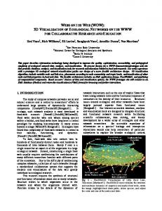
Fig. 1 – 3D Visualization of the food web of Little Rock Lake, Wisconsin (181 nodes and 2375 links). The network shows strong connectivity. Average links per node (in-coming & out-going) is 26.

1

down large networks into smaller subsets may be effective for analyzing local properties, but focusing on such subsets limits more comprehensive understanding of the whole structure. Additionally, species, the nodes within food webs, tend to be closely and highly connected but relatively unclustered. Thus, unlike many other networks, food webs do not display classic “small world” structure [Dun02], which limits the usefulness of visualization strategies based on clusters or compartments (Figure 1). Food webs are much more highly connected than large networks usually found in information visualization (Table 1). Strong connectivity results from each basal (i.e., plants) or “grandchildren” nodes being connected with multiple “children” nodes above, which in turn are connected to multiple “parental” nodes at higher trophic levels. There can also be many connections between children and also between parents. With such high connectivity, edge density, and crossing prevent networks from being clearly or intuitively rendered in 2D. In 3D, graph layout and node placement algorithms can provide more insight by using the additional dimension to minimize occlusion when viewed from multiple viewpoints. In this paper, we discuss visualization of highly connected networks using ecological food webs as an example. Our algorithm responds to network structure and takes advantage of domain specific knowledge to intuitively layout the network for food-web researchers. We are developing these food-web visualizations in conjunction with analysis and database components that include a central data repository for food-web data for collaborative research and education. The importance of food-web network studies and issues of 3D visualization on the WWW are discussed in section 2. Algorithms and the results of graph layout, clustering, and analysis using color schemes and histograms are explained in section 3. Section 4 explains system architecture with a focus on visualization components of the repository system. Section 5 discusses ongoing and future research.

The study of ecological networks, particularly in the form of food webs, has been and continues to be a central paradigm for research into the relationships between ecosystem complexity and stability. A food web describes the network of feeding interactions among taxa within a particular habitat. Quantitative approaches have been used to describe general aspects of food-web network structure, dynamics, and stability since the 1970’s [May73]. Efforts are now underway to integrate realistic ecological network structure with nonlinear dynamics for complex, diverse food webs [Bro03]. While it was relatively easy to depict aspects of early species-poor food-web data with hand drawn 2D wiring networks, such images did little to augment analytical aspects of ecological research. The species diversity, complex network structures, and dynamics that characterize current food-web data and research require a much more sophisticated approach to visualization. Because of the complexity of the data, a visualization framework that abstracts and illustrates food-web network structure and dynamics can play a critical role in understanding, explaining, and predicting important aspects of biocomplexity. 2.2. 3D Visualizations on the WWW Central repositories for a wide range of scientific data have been extremely important for many research endeavors, for example in genomics and paleobiology. Data compiled in centralized repositories can play an important role in ecological research and the conservation and management of ecosystems because no single researcher is an expert in all, or even most of the organisms found in any particular habitat. The integration of analysis and visualization tools with centralized data repositories can dramatically increase the utility of databases and thus increase voluntary use, participation, and collaboration among dispersed researchers, as well as facilitating community inspection and validation of data and theory. Due to the high connectivity of food webs compared to many other kinds of networks, 3D visualization and animation is likely to attract researchers to a central repository by helping researchers gain new insights and develop new hypotheses regarding the structure and dynamics of complex food webs. When providing 3D visualization on the WWW, a central issue includes 3D format selection for universal acceptance due to the lack of 3D standardization on the WWW. Unlike images such as gif or jpg formats that are supported by all WWW browsers, 3D formats are not natively supported. There are different advantages and disadvantages among different approaches such as VRML/X3D, Java Applet/Java Web Start with JOGL, MPEG4, and proprietary Plug-ins [Yoo04]. Considering that the goal of this project includes reaching as many researchers as possible and as well as serving as an

2. BACKGROUND 2.1. Ecological Network Research Graph [Wil99] Fig.7

Average link per node 2.035

Number of nodes(S) 167

Number of links(L) 172

Connecti vity (L/S2) 0.0061

[Her00] Fig.1

1.981

219

218

0.0045

[Her00] Fig.7

1.955

289

291

0.0034

Broom web El Verde web

4.805 19.358

154 156

370 1510

0.0156 0.0620

LittleRock Lake web

26.243

181

2375

0.0724

Table.1 Food web graphs have highly connected nodes compared to nodes in other graph.

2

educational tool, our approach is to support the different preferences of individuals by generating diverse formats with minimal overhead, allowing individuals to make the choice of preferred format. At the same time, we plan to experiment and study performance and usability issues of different 3D formats on the WWW to contribute to web3D standardization. To support diverse formats with minimal overheads, we have developed XML applications to describe visualization data (FoodWebML) as well as graphics user interfaces (GUIML). Streamability, data cache, client-server task separation, XML applications, and flexible pipeline architectures are briefly discussed in section 4.

3. VISUALIZTION AND ANALYSIS Food webs are fundamentally characterized as a set of nodes with links that connect the nodes. In this case, the nodes represent species (or groups of species) and the links represent feeding interactions, and are often referred to as “trophic links.” Trophic links occur between consumer species and the resource species that they eat. Thus, a food web consists of L directed trophic links between S nodes. There are S2 possible and L actual links, so connectance (C) is computed as the fraction of all possible links that are realized (L/S2) and represents a standard measure of food web complexity (Table 1). Some of the key food-web properties that researchers analyze include the fractions of species at top, intermediate and basal trophic levels; the means and variabilities of generality (the number of taxa a species eats), vulnerability (the number of taxa that feed on a species), and food-chain length; the fractions of species that are cannibals, omnivores, and participate in looping; and the degree of trophic similarity between species. These properties of food webs can be derived from relations of species and their binary links and do not depend on additional, non-topological information. The node placement computing component is easily implemented as a “plug & play” in the whole visualization system. Therefore, the visualization system may be easily applied to other highly connected networks.

Fig. 2 Node placement in X axis in each trophic level. ( Y axis ). Radius (depth) is determined by connectivity. Nodes are shown in projection of cylinder.

The Vertical axis (y) is aligned using the convention that species that eat no other organisms are basal species and are at trophic level one, while their direct and indirect consumers are at higher levels, representing the trophic level of the species. Many methods for computing trophic levels exist in the ecological literature. We use the prey-averaged trophic level recently shown to be a computationally efficient algorithm for use within binary food webs [Wil02]. Radius (r) is related to the number of connections attached to the node. This choice of radius places nodes that are less highly connected near the front periphery of the visualization, while more highly connected nodes are placed towards the core of the visualization. In systems with a large number of links, placing less connected nodes towards the front of the visualization allows more of the network structure to be seen. The θ value is used for placing closely related nodes next to each other. In food webs, one meaningful relation is a predating behavior, so we place species that are predated by a same node close together. This algorithm provides two advantages. First, total link length has been reduced up to 43%, with an average reduction of 33%, compared to random placing. Obviously visual cluttering is also reduced. Second, it is easy to recognize relations between prey and predators by focusing on locality [Yod98] of interactions in the food webs and deriving inherent structures of the network. Relative niche position in ecosystems can be revealed and species easily recognized from link patterns and node position, even without annotation.

3.1 Graph Layout/3D Node Placement We represent nodes (species) as spheres and links as cones, with the cone tapered from predator to prey. We experimented different coordinate systems to represent food webs, but a cylindrical coordinate system (with coordinates r, θ, y) generates the most intuitive structure due to our natural familiarity with food chains associated with the vertical axis.

3

Before Aggregation

Similarity Coefficient = 1

Similarity Coefficient = 0.75

Similarity Coefficient = 0.5

Similarity Coefficient = 0.25

Fig. 3. Hierarchical aggregation of Little Rock Lake food web by trophic similarity is shown. Aggregation rate in each food web is determined by similarity coefficient. The predating behavior algorithm has two elements. First, it identifies groups of nodes in each trophic level and then merges groups that share common species, allowing close placement of predator species. Figure 2 shows prey A and its predators a, b, c and prey B and its predators c, d, and e. They can be grouped to A (a, b, c) and to B (c, d, e). After the initial grouping, groups A and B are merged to group AB (a, b, c, d, e) so that predator nodes can be placed closely later. We iterate the process till no groups share the same components. Second, it places group of nodes at each trophic level. Placement of predator nodes uses a radial layout algorithm that was inspired by the visualization method for large hierarchies [Wil99] as shown in Fig. 2.

the amount of trophic overlap between taxa. A trophic overlap similarity index (I) between every pair of nodes is calculated using an algorithm defined by Jaccard [Mar91]: I = c/(a+b+c) where c = number of predators and prey common to the two nodes, a = number of predators and prey unique to one node, and b = number of predators and prey unique to the other node. When the two nodes have the same set of predators and prey, I = 1. When the two nodes have no common predators or common prey, I = 0.

The clustering algorithm used for trophic species is used to reduce methodological variation among datasets with uneven resolution of species, and is a purely structure-based clustering which uses only nodes and link information for calculation. In the algorithm, a prey link is an incoming directed link, and a predator link is an outgoing directed link. This can be easily extended to different applications involving networks with binary link relations. Visualization results with different coefficients are shown in Figure 3. We scaled up nodes and links to represent clustering.

3.2 Aggregation/Clustering Clustering is important for large or complex networks not only to reduce visual clustering for better navigation, but also to organize nodes into meaningful clusters and add analytical intuitiveness. Clustering species by tropic similarity helps ecologists to investigate resolution-related issues in statistics commonly used to describe food-web patterns. To cluster species in the raw food web, the nodes are hierarchically clustered based on

3.3 Analysis with Node Colors Since human perception responds strongly to color,

Parasites Top predators

Fig.4.a. Taxonomical color on Broom food web. Fungi kingdom (yellow), Monera (red), Animala (blue), and Plantae kingdom (green) are shown.

Fig.4.b. Vulnerability color on Elverde food web. Histogram shows slots indexed from 0 to 45 (not continuous). The index represents the number of species that are eating the species under the specific index.

4

a certain property, the advantage is that a single color tint gives good visual cues of the distribution of the property, while multiple colors usually do not convey sequential ordering. The disadvantage is that a single color tint has a limited number of distinguishable tints. To choose tint levels to be smoothly distributed and at the same time as distinct as possible, tint distribution is calculated by bucket sizes. The bucket size is calculated by the number of nodes divided by the number of tint levels. A histogram of bucket sizes is added to the left side of the screen to assist understanding of the tint distributions. In Figure 4b, most nodes in the top position along the Y axis have bright tints because they are top predators, but some of the nodes at the top position have dark tints. They turn out to be parasite species which live in or on high trophic level predators.

manipulating color has been a popular approach in information visualization. However, it has not been intensively utilized in network visualization, perhaps because there may be limits to the amount and diversity of information that can be usefully displayed and perceived at one time [McG02]. With food webs, we tried to use color schemas that complement 3D structures to create effective visual aids. For example, node color varies with the trophic level of the node. Link color also varies with the trophic level of the prey species. This means that omnivores, or species that consume prey from more than one trophic level, are easily picked out because of the large diameter end of links of different colors that connect to a single node. Vulnerability and Generality Color Vulnerability describes how many predators a species has, and generality describes how many prey items it eats. The sum of vulnerability and generality gives the “degree” of each mode, or the total number of links to or from a particular species. The degree of a species is important for studying the likelihood of cascading extinction from biodiversity loss [Dun02]. We experimented representing vulnerability and generality using the Radius (r from the cylindrical coordinates) of node but the properties were not easily comprehensible this way, compared to color. The number of slots in the histogram of vulnerability for a food web shown in Figure 4b is decided by unique numbers of predators of single species. For example, for this food web slots are indexed from 0 to 45 (not continuous). The index 0 represents species that have no predators, which are either top predators or parasites that are not themselves parasitized. Index 45 includes species that have 45 predators, and thus have high vulnerability, and probably high degree. When visualizing vulnerability, we use tint distribution instead of multiple colors. When linear tint distribution of a single color is used to sequentially index

(a)

Taxonomic Color Comparing trophic and taxonomic characteristics may provide interesting insights to ecologists. This comparison can be conducted visually by seeing how closely related species are placed and grouped after accounting for predator behavior. This function allows users to examine not only locality but also taxonomic distribution of nodes in multi-resolution/hierarchical taxonomic levels. Coloring can be done at the level of Family, Order, Class, Phylum and Kingdom (Figure 4a shows taxonomic coloring at the Kingdom level while Figure 5a shows coloring at the Order level). Too Many Colors and Shapes We experimented showing multiple colors on a node at the same time when a node has many attributes to be presented. as a means for maximizing analytical efficiency. For example, we used the top face for trophic level color, a side faces for vulnerability, and a side face to display an image of the species. Alternatively, using a box to denote a node, instead of a sphere, can allow ordered representation of additional

(b)

(c)

Fig. 5 (a) Annotations of species name are shown in green color on nodes selected by user. (b) shows depth cue in Little Rock Lake web (c) shows node search results of Scotch Broom web that node which has more than 2 prey is high-lighted; Other nodes and links are gray-scaled

5

dimensions (six total) of information. But the feedback from users about the box nodes was not favorable since too much information kept them from seeing more coarse-grained information network relationships. From a cognitive perspective, the level of human understanding increases proportionally with the amount of information only up to certain level [Her00]. Therefore it is important to balance between the amount of information provided and the ability of humans to perceive that information. We also provide an additional depth cue. Since the visualization is based on cylindrical coordinates, we use layers of circular disks to enhance the depth cue of node positions in 3D and advance search (Figure 5b and c).

We are currently developing a semantic web data bank for food webs, and are developing the interface between the data bank, the visualization pipeline, Java client using JOGL and Java Web Start, and GUIML. When the GUIML and Java client are completed, we plan to do a usability study using surveys on 3D network visualization and formats on the WWW. Due to the lack of standards for web3D, the usability study will contribute to developing such standards for the WWW and embedded systems. Many other attributes of food webs and their visualization and analysis are being studied. Ultimately, the system will be extended to other application areas. Animations and simulations will be added for research and educational purposes.

4. WOW ARCHITECTURE DESIGN

ACKNOWLEDGEMENT This project is being funded by National Science Foundation Div. Of Biological Infrastructure, Biological Databases and Information, No. DBI-0234980.

FoodWebML XML serves well for heterogeneous database description. In our approach, FoodWebML is used to describe the ontology of food-web data and it also contains intermediate or final visualization components as a cache. When visualization is being processed through the pipeline, intermediate data such as trophic levels or visual information node properties (color, size, geometry, position) are computed and saved back to FoodWebML, so they can be easily reused in the future given any changes in food-web data. FoodWebML contains contents and presentations (visual info) in one XML application, but they are clearly separated internally. Visual nodes within FoodWebML can be easily translated to X3D/VRML. When used with Shockwave Lingo, visual nodes are sent out in a streaming fashion, so clients receive nodes and links closer to the viewer, which are rendered while the rest arrives and is updated [Yoo04].

REFERENCES [Aub03] Auber,D., Chiricota, Y., Jourdan, F. 2003. Multiscale Visualization of Small World Networks. IEEE Information Visualization 2003 [Bro03] Brose, U., Williams, R.J., & Martinez, N.D. 2003. Comment on “Foraging adaptation and the relationship between food-web complexity and stability.” Science 301:918. [Dun02] Dunne, J.A., Williams, R.J., & Martinez, N.D. 2002. Food web structure and network theory: the role of connectance and size. Proceedings of the National Academy of Sciences USA 99:1291712922. [Fre00] Freeman, L.C. Visualizing social networks. Journal of Social Structure 1. 2000. [Gar03] Garlaschelli, D., G. Caldarelli, & L. Pietronero. 2003. Universal scaling relations in food webs. Nature 423:165-168. [Her00]Herman, I., Melancon, G., & Marshall, M., Graph Visualization and Navigation in Information Visualization: A survey. IEEE Transactions on Visualization and Computer Graphics. 2000. [May73] May, R.M. 1973. Stability and Complexity in Model Ecosystems. Princeton University Press, Princeton, N.J. [McG02] McGrath, C., Krackhardt, D., Blythe, J., Visual complexity in networks: seeing both the forest and the trees. Connections, (25) 1: 30-34, 2002 [Mar91] Martinez,N.D. Artifacts or attributes effects of resolution on the Little Rock Lake food web. Ecol. Monog 61:367-392. 1991 [Str01] Strogatz S.H. Exploring complex networks. Nature, 410 268275, 2001. [Wil99] Wills, G. NicheWorks—Interactive Visualization of Very Large Graphs, Journal of Computational and Graphical Statistics 8, pp 190-212. 1999 [Wil00]Williams, R. & Martinez, N.D. Simple rules yield complex food webs. Nature 404, 180 - 183 (2000) [Wil01] Williams, R., & Martinez, N.D., Stabilization of chaotic and non-permanent food web dynamics. SFI Working Paper. 2001, [Wil02] Williams, R., & Martinez, N.D. Trophic Levels in Complex Food Webs : Theory and Data. 2002 SFI working paper [Yod98] YODZIS, P. Local trophodynamics and the interaction of marine mammals and fisheries in the Benguela ecosystem. Journal of Animal Ecology 67:635-658. 1998 [Yoo04] Yoon, I., Williams, R., Levine, E., Yoon, S., Dunne, J., Martinez, N.D. Webs on the Web: 3D Visualization of Ecological Networks on the WWW for Collaborative Research and Education. SPIE Electronic Imaging conference, 2004.

Visualization Pipeline Our current pipeline stays on the server side. While processing a visualization, FoodWebML stores intermediate data as a cache within the pipeline and the resulting visualization information is sent to the client according to the format that user wants. This approach is efficient, especially during frequent access to the same food web, via reuse of up-to-date cache information. An alternative is moving the visualization pipeline to the client side where the client receives only food-web data and conducts intensive analysis and visualization without any connection to server. Both approaches are supported with the current server pipeline. We are developing a java version client using JOGL and Java Web Start as a thick client for intensive users. Our server side pipeline is easily ported to the client side.

5. DISCUSSION AND FUTURE WORK

6

7