Ocean Sci., 10, 701–718, 2014 www.ocean-sci.net/10/701/2014/ doi:10.5194/os-10-701-2014 © Author(s) 2014. CC Attribution 3.0 License.
Weighing the ocean with bottom-pressure sensors: robustness of the ocean mass annual cycle estimate Joanne Williams1 , C. W. Hughes1,2 , M. E. Tamisiea1 , and S. D. P. Williams1 1 National 2 School
Oceanography Centre, Joseph Proudman Building, 6 Brownlow St, Liverpool L3 5DA, UK of Environmental Sciences, University of Liverpool, Liverpool L69 3GP, UK
Correspondence to: Joanne Williams (
[email protected]) Received: 10 October 2013 – Published in Ocean Sci. Discuss.: 5 February 2014 Revised: 27 June 2014 – Accepted: 2 July 2014 – Published: 11 August 2014
Abstract. We use ocean bottom-pressure measurements from 17 tropical sites to determine the annual cycle of ocean mass. We show that such a calculation is robust, and use three methods to estimate errors in the mass determination. Our final best estimate, using data from the best sites and two ocean models, is that the annual cycle has an amplitude of 0.85 mbar (equivalent to 8.4 mm of sea level, or 3100 Gt of water), with a 95 % chance of lying within the range 0.61– 1.17 mbar. The time of the peak in ocean mass is 10 October, with 95 % chance of occurring between 21 September and 25 October. The simultaneous fitting of annual ocean mass also improves the fitting of bottom-pressure instrument drift.
1 Introduction The total mass of water in the oceans fluctuates with seasonal changes in continental water storage. A measure of the annual cycle of water exchange is of widespread interest and has been estimated in at least nine studies using data and models including satellite gravity, hydrology, ocean steric height and satellite altimetry. Amplitude estimates have a wide range of 5.5–9.4 mm (Vinogradov et al., 2008; Wouters et al., 2011), and phases from 259–303◦ (Siegismund et al., 2011; Rietbroek et al., 2009). (A phase of zero represents an annual peak at the start of the year, so these correspond to a maximum ocean mass between 19 September and 3 November.) It is theoretically possible to use a single bottom-pressure sensor to monitor changes in the total mass of water in the oceans independently of satellite gravity measurements and, if the sensor location is carefully selected, with little
dependence on hydrology models (Hughes et al., 2012). There is also a great deal of interest in monitoring interannual or decadal variations and long-term trends in ocean mass, but existing bottom-pressure sensor technology makes this extremely difficult, as the instruments, usually deployed for high-frequency tasks such as tsunami monitoring, suffer from non-linear drift of the order of centimetres per year. The drift can vary even between redeployment of the same instrument (Watts and Kontoyiannis, 1990; Polster et al., 2009). However, a good determination of the annual cycle of ocean mass change is still valuable for constraining models of hydrology and ocean dynamics, and in providing an independent measurement for comparison with GRACE and altimetry. Conversely, knowledge of the annual cycle also allows us to improve estimates of the non-linear contribution to bottom-pressure instrument drift. Based on a pair of bottom-pressure sensors moored in the Pacific, Hughes et al. (2012) estimated an amplitude 8.5 mm (equivalent to a global average pressure of 0.86 mbar, or about 3200 Gt of water) and phase 262◦ (22 September). This lies within the envelope of results from other studies, but no formal attempt was made to put error bounds on this number, although it was noted that a similar value could be derived using different ocean models. Ocean dynamics aside, the bottom-pressure cycle measured at a given site is affected by the crustal deformation and gravitational effects caused by the mass change on land. The bottom pressure needs adjusting everywhere to derive the global ocean mass change, but at certain sensor locations in the central Pacific the result is uniformly biased high. At these locations the effect on local bottom pressure is almost independent of the origin of the additional water mass, which
Published by Copernicus Publications on behalf of the European Geosciences Union.
702
Joanne Williams et al.: Error estimates on weighing the oceans
could equally come from Greenland, Antarctica or the Amazon. This was the reason for the choice of sites S and N of Hughes et al. (2012), as the nearest existing data to the optimal region. In this paper, we will apply the Hughes et al. (2012) “weighing” technique to existing bottom-pressure data from 17 moorings (including sites S and N) at tropical sites around the world. Many of these represent sites that would not be considered ideal, either due to increased variance of the dynamic bottom-pressure signal or dependence upon the specifics of the continental hydrology. We use ocean models to remove local dynamics, including self-attraction and loading corrections. We use long-period tide models and atmospheric pressure data to correct for those components omitted from ocean models. We will first, independently of any hydrology model, show the range of annual cycles in local pressure that arise from mass exchange, and how the error bounds vary between sites according to the quality of available data. Then, with an hydrology-and-atmosphere model based on GLDAS (the Global Land Data Assimilation System, Rodell et al., 2004), we account for the expected differences between sites and make use of data from these sub-optimal locations, reducing error bounds on the predicted annual cycle of global ocean mass. We will describe three techniques to derive error estimates, and how to combine data from multiple sites. Our best estimate is that the ocean annual cycle has an amplitude of 0.85 mbar and phase of 280◦ (10 October), with 95 % of results within 0.61–1.17 mbar or 261–294◦ (21 September– 25 October). 2 2.1
Calculating annual cycle in bottom pressure at the 17 sites individually: method Contributions to bottom pressure
The bottom pressure prec measured by a given sensor can be decomposed as prec = pdrift + pdyn + pt + pa + pm ,
(1)
where pdrift is sensor drift, pdyn is the change due to ocean dynamics, pt is due to tides, pa is the atmospheric pressure averaged over the ocean and pm is due to the change in ocean mass due to precipitation, evaporation, grounded ice melt and river runoff. Some function Fs relates the global-average mass change mo to the pressure felt at an individual site. In general, Fs , an adjustment due to the changing geoid and crustal loading, is dependent not just on the site location but on the distribution of ocean and continental water mass, and cannot be assumed to be stationary. However, for the annual component we may assume that such a uniquely invertible function exists for a given site, pm = Fs (mo ). Ocean Sci., 10, 701–718, 2014
(2)
In this part of the paper we seek only to determine the annual cycle of the local pressure pm at each site, and not mo itself. This annual cycle of pm is calculated completely independently of any hydrological or atmospheric model, or GRACE data. In Sects. 4 and 5 we will employ a hydrological and atmospheric model to determine Fs at annual timescales for each site – a rather small correction, at certain sites – and hence the annual cycle in ocean mass. 2.1.1
Sensor locations
For this paper, we use data from the US National Tsunami Hazard Mitigation Program (González et al., 2005), downloaded from http://www.ndbc.noaa.gov/dart.shtml. These were, at the time of selection, all the sites available in the open ocean within 18◦ of the equator with records from 2001 onwards. Where records have been converted to equivalent metres of sea level, we revert them to pressure in mbar using the original conversion factor. There are 17 sites, at locations shown in Fig. 1 and Table A1. Sites 17 and 11 correspond to sites N and S of Hughes et al. (2012). These two sites are the earliest, starting in September 2001 and January 2003 respectively; the other sites have deployments between 2006 and 2011. At most sites there are multiple instrument deployments. The deployments varying in length from a few months to over 2 years, and there are many gaps in data both between and during deployments. Sites 3, 8, 9, and 16 have particularly short records. We initially do an approximate detrending, in order to fit and remove tides with daily or shorter periods and the fortnightly tide components Mf and Msf with periods 13.66 and 14.77 days. Then we replace trends ready to calculate a more precise drift fit in combination with the annual signal, as described in Sect. 2.2. The data with fortnightly and shorter tides removed is shown in Fig. 2. 2.1.2
Long-period tides
There remain other tidal constituents with monthly or longer periods in pt which can be removed by modelling rather than fitting, and thus avoiding contamination by the sensor drift. (In fact we tried both fitting and modelling for removing fortnightly and monthly equilibrium tides, and found less than 0.01 mbar difference in results for the annual cycle.) The first of the long-period tides we consider is the Pole Tide ηp , which arises from variations in the apparent location of the Earth’s rotational axis, and hence variations in the centrifugal potential. It has main periods of 12 and 14 months and amplitudes of up to 0.7 mbar at the bottompressure recorder sites. We calculate this using the derivation given by Desai (2002). Over the ocean, ηp = px E(ηx ) − py E(ηy ),
(3) www.ocean-sci.net/10/701/2014/
Joanne Williams et al.: Error estimates on weighing the oceans
703
Figure 1. Locations of test sites and bathymetry from Nemo 1/12◦ model.
where
and the coefficient z0 corresponds to the components with periods 18.6 years, annual, semi-annual and 4-monthly, and z1 , z1a to monthly components. The time series for z0 , z1 and z1a are synthesised using components tabulated by Cartwright and Tayler (1971); Cartwright and Edden (1973).
ηx = −3.856 sin(2φ) cos(λ), ηy = −3.856 sin(2φ) sin(λ), in mbar, for longitude λ, latitude φ. The function E is the correction to η due to self-attraction and loading, and is explained below. The components px , py are the tilt of the pole in arcseconds taken from the EOP (IERS) 08 C04 data set of Earth orientation parameters, from the International Earth Rotation and Reference Systems Service. (Note that the IERS defines y along 90◦ W, hence the negative coefficient). We subtract a constant and linear trend from px , py , in order to focus on shorter period signals. There are also long-period equilibrium tides with amplitude of up to 1.5 mbar over the recorder sites. These are of the form ηlp = (z0 (t) + z1 (t))E(ηc ) + z1a (t)E(η3 ), where ηc = 3 sin2 φ − 1, η3 = 2.5 sin3 φ − 1.5 sin φ, www.ocean-sci.net/10/701/2014/
(4)
2.1.3
Self-attraction and loading of long-period tides
The presence of additional water causes crustal deformation and geoid changes that change the ocean depth, both locally and globally. Generically, loading effects such as these are sometimes referred to as self-attraction and loading (SAL). So as well as the effect of the external changes in gravitational potential, we account for SAL corrections to the longperiod tides. We do this following the method using Green’s functions described by Stepanov and Hughes (2004). To calculate E for each η we apply the technique described by Agnew and Farrell (1978), who applied it to an input potential equivalent to our ηc . The ocean at a point (φa , λa ) feels the effect of the sea-level change at each other point, η(φb , λb ), according to a function G(α) where α is the angular distance between a and b. We assume that the additional mass at the point (φb , λb ) due to the sea-level change η(φb , λb ) is Ocean Sci., 10, 701–718, 2014
704
Joanne Williams et al.: Error estimates on weighing the oceans
Figure 2. Bottom-pressure data from the 17 test sites (mbar, offset for clarity), following subtraction by least squares fitting of tides with periods of fortnightly and shorter. Stars indicate the start of sensor deployments. There may be gaps in data within deployments. Black squares indicate convergence warnings in the drift fitting. These are not necessarily on the shortest deployments. The overlaid green line shows the sensor drift fitted using the iterative technique on all sites simultaneously. The end dates of the ocean models are also indicated. The y-axis offset between sites is 15 mbar.
distributed in a circular cosine bell hump, i.e. mass is proportional to (1 + cos(πr/rx ))/2 where r is the arc length of α and rx = 0.25◦ is chosen as the grid size. G has three components, G = G1 + Gk − Gh , which are the Green functions for vertical seafloor displacement due to loading, Gh ; vertical geoid displacement due to indirect attraction, Gk ; and vertical geoid displacement due to direct attraction of the load, G1 . These are taken from interpolations of the Green functions given by Francis and Mazzega (1990). We integrate the attraction over all points b to give the global function E(η), the additional mass at any point due to the input sea level η: Z E(η(a)) = η(a)G(α(a, b)) db. ocean
Then, since the correction E(η) itself changes the geoid, the process must be iterated. Eventually we converge on ηtot (φ, λ), an equilibrium response to the forcing by the spherical harmonic η, which is self-consistent under loading Ocean Sci., 10, 701–718, 2014
and self-attraction, so ηtot ≈ E(ηtot ) = E(η). This is done for η = ηx , ηy , ηc and η3 , and the result is consistent with the maps of Agnew and Farrell (1978) for ηc and Desai (2002) for ηx and ηy . The process only slightly changes the analytical functions calculated without applying the SAL correction, in most areas scaling them by about 1.25. 2.1.4
Ocean dynamics and atmospheric pressure
To remove the local ocean dynamics pdyn from the bottompressure measurements, we use ocean models. For this study we have available five models, as detailed in Table 1. ECCO and the 1/12◦ NEMO runs provide the best overlap with the bottom-pressure data, and results below are based on ECCO unless stated otherwise. We subtract the global spatial average of bottom pressure at each time from the model data, to remove any added mass, as well as removing artifacts due to the model’s Boussinesq approximation. Figure A1 shows the annual cycles of local bottom pressure that are found in the models at each site, with most sites www.ocean-sci.net/10/701/2014/
Joanne Williams et al.: Error estimates on weighing the oceans
705
Table 1. Ocean circulation models used in this study. Model
Resolution
Start date
End date
ECCOa
1/4◦
OCCAMb OCCAM NEMOc NEMO
1/4◦ 1/12◦ 1/4◦ 1/12◦
1992 1985 1988 1959 1979
2010 2003 2004 2007 2010
a ECCO data is the 18 km resolution ECCO2 model with data
assimilation from Jet Propulsion Laboratory (Menemenlis et al., 2005), b OCCAM data from National Oceanography Centre, run 202 at 1/4◦ and run 401 at 1/12◦ (Marsh et al., 2009), c NEMO data from National Oceanography Centre, runs ORCA025-N206 and ORCA0083-N001 (Blaker et al., 2014).
having an amplitude of about 0.5–1 mbar. At some sites (e.g. 11) the models give consistent annual cycles, but at site 2 there is almost a factor of 2 difference in amplitude between ECCO and NEMO 1/12◦ and at site 17 there is a range of 76◦ between OCCAM 1/12◦ and NEMO 1/12◦ . This is one of the greatest areas of uncertainty in this study. The atmospheric pressure averaged over the global ocean, pa , needs to be removed from the bottom-pressure record, and this is done using the ECMWF analysis data set provided as a satellite altimeter product by Aviso. pa has an annual amplitude of 0.61 mbar and phase 186◦ , peaking at 7 July. 2.1.5
Self-attraction and loading of dynamic pressure
The ocean models assume a constant gravitational field and ocean floor, but in the real world water masses cause crustal deformation and changes to the geoid as described above. For the pdyn component, we correct the model data for these SAL effects, in a similar way to the calculation by Tamisiea et al. (2010). The SAL correction to the dynamic pressure from model data has an annual amplitude of up to 0.2 mbar at these sites. This correction was not made in the previous study (Hughes et al., 2012) and accounts for a large part of the phase difference between that study and this one. 2.2
Removing non-linear sensor drift
Currently available bottom-pressure sensors suffer from drift that can be larger than the annual cycle of bottom pressure (Fig. 2). We follow Watts and Kontoyiannis (1990) and Polster et al. (2009) in assuming that the drift is an initial decaying exponential and a long-term linear, that is of the form pdrift = a1 + a2 τ + a3 e−τ/|a4 | , where τ is the time in days since the start of the deployment. To prevent our fitted drift absorbing the annual cycle (we cannot prevent it absorbing the long-term trend without further information on instrument drift), we use an iterative process ANN + p as follows. We write pm = pm noise , i.e. the annual signal we seek plus some signal which includes high frequency www.ocean-sci.net/10/701/2014/
Figure 3. Drift fitting to site 15. The yellow line is the fit to the raw bp record (blue), without taking account of the annual mass signal or other corrections. Green is the iterative fit to just that site, and magenta is the fit with the annual fitted to all sites simultaneously (discussed later).
ocean mass changes and errors in the ocean model. Rearranging Eq. (1) as ANN pres = pdrift + pnoise = prec − (pdyn + pt + pa + pm ), ANN (we start with amplitude = 1 mbar, phase = 0) we guess pm and find coefficients to fit pdrift to pres . If we have correctly ANN , then there will be no annual signal in the guessed pm ANN1 to dedrifted residual pnoise . So we fit another annual pm ANN pnoise , and use this to adjust our estimate of pm . We iterate ANN and the drift fit, until there is no with fresh attempts at pm ANN has converged. Converannual signal left in pnoise , and pm gence to a tolerance of 0.005 mbar (amplitude of adjustment between iterations) is usually achieved within about 10 iterations; “no convergence” is declared after 80 iterations. For most sites in our test set, there is more than one deployment, although there may be gaps between and during deployments. In these cases the iterative procedure involves all deployments at a site, simultaneously fitting individual drifts and a single annual cycle. An example of the fitted drift is shown in Fig. 3.
3 3.1
Calculating annual cycle in bottom pressure at the 17 sites individually: results Requirement for iterative fit for dedrifting
Figure 4 shows the fitted annual cycle of bottom pressure at each site when the recorder drift is calculated (a) with the iterative procedure outlined above and (b) with a least-squares fit of an exponential-plus-linear to the raw recorder data prec . At some sites (1, 2, 4, 10, 11 and 12) the iterative fitting Ocean Sci., 10, 701–718, 2014
706
Joanne Williams et al.: Error estimates on weighing the oceans
ANN predicted using iterative fitting; (b) local Figure 4. Phasor diagrams for annual cycles at each site, for: (a) local bottom pressure pm ANN predicted without iterative fitting (sites 3 and 8 are outside the axes); (c) local pressure p and global ocean mass m bottom pressure pm h h predicted by two hydrology models: GLDAS-1 is shown with stars (ph ) and cross (mh ), GLDAS-2.0 with squares (ph ) and diamond (mh ); (d) global ocean mass mo , using a hydrology model GLDAS-1 to provide Fs . Axes for (c) are indicated by red box on (a). All converged sites are included, some have large error bounds to be described below.
makes fairly small differences, but the fitted annuals at sites 5, 13, 14 and 15 are changed substantially. Site 15 provides a particularly clear example (see Fig. 3). The apparent decrease of the bottom-pressure record in late 2008 is due to the coincidence of the annual ocean mass decrease. The drift fitted to the raw data is 21.54 − 0.05τ − 47.47e−τ/84.33 , which is decreasing at the end of the record. The iterative fit allows for the sinusoidal contribution of the ocean mass and other variables, and the resulting drift is −3.76 + 0.05τ − 19.41e−τ/37.24 , increasing throughout the record. Using the raw-data drift fit would result in a bottompressure error of over 3 mbar for the end of the record. With a differing sign for the linear part, serious error could result from any extrapolation of the raw-data drift fit.
Ocean Sci., 10, 701–718, 2014
This removal of a real pressure signal occurs for the first deployment of sites 13, 14, and 15, all of which are only 16 months long and finish in April 2008 at the minimum of the ocean mass cycle, maximising the risk of the annual signal contaminating the drift fit to the raw data. For the first deployment at site 13 the raw fit is over 6 mbar too low at the end of the record. It is worth remembering that we have not attempted to distinguish between the bottom-pressure recorder drift and any long-term trends in ocean mass. So this fit represents a combination of recorder drift and any trend or variability in ocean mass longer than 1 year. Trends in other components of Eq. (1) may also remain.
www.ocean-sci.net/10/701/2014/
Joanne Williams et al.: Error estimates on weighing the oceans 3.2
Range of results across test sites
ANN for The amplitude and phase of the annual cycles in pm each of the test sites is shown in Fig. 4a, plotted with a phase of zero at the top representing an annual peak at the start of the year. Site 11 (S) has amplitude 0.93 mbar and phase 272◦ peaking at 3 October, slightly larger and later than the result of Hughes et al. (2012) for the combination of sites S and N. For sites 3, 8, 9 and 16, all of which had very short deployments, the iteration did not converge. At this stage, some of the results differ wildly from other measurements of the ocean annual cycle, with a scatter of 6 months of phase and several times amplitude. They are not expected to be exactly the same as these are measureANN ) at each site, with ments of residual pressure cycle (pm geographic variation in ocean mass still included, i.e. the inverse of the function Fs still to be applied to convert to global average ocean mass mo . But it is clear that the scatter is larger than that predicted by the ocean mass model (Fig. 4c). It is perhaps not surprising that the short deployment at sites 4 and 5 produced implausible results, but more so that there is so much difference between neighbouring sites 13 and 15. However, we have yet to examine the error bounds on these measurements and as we will see in following sections, the bounds on some sites are much larger than on others.
3.3
707
spectral index is therefore estimated from the power spectra to be around −1.8. We simulate the noise using the discrete simulation method described by Kasdin (1995) where the impulse response function is created to mimic the −1.8 spectral index at high frequencies and −1.3 index at periods greater than 2 days. Finally, to recreate the flattening at low frequencies we also remove trends from the simulated data for randomly sized segments equivalent to that seen in the real data. We do not create any extra power at tidal frequencies. We then adjust each of the 17 original bottom-pressure signals using prec − pnoise + pnoise1 – the same pnoise1 for every site – and redo the iterative drift and annual fit. This is repeated for 100 noise signals to give a spread of results for each site. Although the models perform better at some sites than others, the same noise spectrum is used for each site. This enables us to directly compare the spread of results at one site with another. Figure 5 shows the scatter of the resulting annual fits for each site. For sites 3, 8, 9 and 16 only a few results are plotted, this is not necessarily because the amplitude is greater than the range shown but because the iterative fit diverged. The fits with a close grouping, such as 1, 2, and 11, are those for which the annual fit has been robust to the specific noise estimate. Some of the surprising results in Fig. 4a, such as sites 4 and 15, are those for which there is a large spread here.
Sensitivity to noise 3.4
If all dynamical signals were perfectly modelled and removed, then it would always be possible to distinguish annual cycles from sensor drift. However, the presence of noise means that our ability to distinguish these two signals will depend in a complicated way on the type and amplitude of the noise, the nature of the drift, and lengths of time series. To test this, we produce a random noise signal pnoise1 with similar frequency spectrum to the residual pres . To produce simulated time series whose stochastic properties closely match the real data we first form the power spectra from the 17 series. Given that the series contains many gaps we use a combination of the Lomb–Scargle periodogram (Lomb, 1976; Scargle, 1982) and Fourier spectral analysis on segments that were over 5000 epochs (52 days) long to produce a good representation of the spectra. We find that the spectra follow a power law shape, that is the power is proportional to f α , for frequency f and spectral index α. However, the slope appears to change at around a period of 2 days and at the lowest frequencies the spectra is essentially flat, probably due to removing the drift from the series. We estimate the low-frequency spectral index (period greater than 2 days) by averaging the series to daily estimates and using maximum likelihood estimation (MLE). All 17 estimates of the spectral index are then averaged to come out with a spectral index of −1.3. We cannot estimate the high-frequency spectral index using MLE because the sub-daily part of the spectrum is biased by remaining power at tidal frequencies. The www.ocean-sci.net/10/701/2014/
Comparison of ocean models
The models for ocean dynamics, NEMO, ECCO and OCCAM, have similar annual cycles of model bottom pressure (pdyn ) for some sites (e.g. sites 7, 10, 11) but agree less well at others (e.g. sites 2, 15) (see Fig. A1). This increases the error bound on the ocean mass for the latter sites, suggesting that more weight should be given to those sites with good model agreement. To calculate this rigorously, we repeat the noise calculation in Sect. 3.3 for all models. These have the distributions as shown in Fig. 6. The OCCAM and NEMO4 models have shorter overlaps with the data, and hence provide shorter series for the annual fitting, which may account for the poorer performance of these models. The OCCAM models are only used at sites 11 and 17. NEMO4 has a short overlap with the data at most sites, but overlaps more than 16 months only at sites 1, 11 and 17. At sites 4 and 5 there are only 14 months of data, insufficient for a reliable estimate of the annual cycle. Site 16 has a long gap between deployments, with only 15 months of data in total. We see that the result at site 1 is consistent between models.
Ocean Sci., 10, 701–718, 2014
708
Joanne Williams et al.: Error estimates on weighing the oceans
ANN for each site with noise added to the bottom-pressure records. Subplot axes are identical to Fig. 4a. Figure 5. Scatter of pm
4
4.1
Calculating annual cycle in ocean mass from the 17 sites individually Spatial variability of mass signal pm
In Sect. 3 we focussed on pm , the annual that can be retrieved from bottom-pressure records once other known signals had been removed: atmospheric pressure, long-period tides and ocean dynamics. Of these, the last is probably the least known and would introduce the greatest spatial variability into the bottom-pressure records. However, even once these “known” signals are removed, hopefully leaving just the pressure signal due to mass flux, we would not expect pm to be globally uniform (e.g. Clarke et al., 2005). During the annual water cycle, some continental locations store large masses of water, and the SAL effects of this additional mass should be accounted for. Ideally, one might locate bottom-pressure sensors far from land, so that the location of the variation of water mass on the continents would be irrelevant. Hughes et al. (2012) demonstrated that no matter the location of the mass change on the continents, areas of the Pacific Ocean experience nearly the Ocean Sci., 10, 701–718, 2014
same change in bottom pressure. They divided the continental areas into 2283 separate regions, and looked at the change in bottom pressure associated with a water loss from each region that would be associated with a one millimetre globally averaged sea level rise. While areas near the mass loss experience a bottom-pressure decrease, a section of the Pacific experiences an increase only ranging between 0.9 mm and 1.3 mm whatever the locations of mass loss on the continents. On average, this region experiences a higher-thanaverage sea level change of 1.15–1.18 mm. Unfortunately, the bottom-pressure records are not located in this ideal area, as coastal locations are more relevant in their role in the tsunami warning system. Thus, we expect that crustal deformation and geoid changes can introduce spatial variations into the amplitude and phase of the annual mass signal. We will now introduce how we account for this when trying to find a globally averaged value. 4.2
Modelling the spatial variability of pm
The change in bottom pressure pm due to the annual cycle of mass change mo , depends upon the location of www.ocean-sci.net/10/701/2014/
Joanne Williams et al.: Error estimates on weighing the oceans
709
ANN derived from different models, for each site. Models are indicated as ECCO (blue), NEMO12 (green), Figure 6. Comparison of pm NEMO4 (red), OCCAM12 (cyan), OCCAM4 (magenta). 95 % of results lie within the contours. No contours are plotted if there is less than 13 months overlap between model and record data at a site. Subplot axes are identical to Fig. 4a.
the bottom-pressure sensor and pattern of mass change on the continents, according to some function Fs . Similar to Hughes et al. (2012), we follow the approach of Tamisiea et al. (2010), using hydrological and atmospheric models to estimate Fs as Fs ≈ ph /mh , where ph is the model prediction of pressure for that site, and mh is the model estimate of mo . The dominant contribution to the ocean mass comes from the change in water storage on the continents. However, the atmosphere also contributes to the global annual cycle in ocean mass, both by storing water mass and by pressure changes introducing loading changes on the continent. In this calculation, we assume that the Earth responds elastically, which is reasonable for the annual cycle. For our primary estimate of this effect, we use the GLDAS/Noah data version 1 (GLDAS-1) (Rodell et al., 2004) over the period December 2001 to November 2010. Since this does not extend to Antarctica, and the data in Greenland should not be used, we add the same component www.ocean-sci.net/10/701/2014/
from GRACE for these regions as used in Tamisiea et al. (2010) and Velicogna (2009), although this has a rather small effect. For the atmospheric data, we use the monthly-mean surface pressure fields from the National Centers for Environmental Prediction/National Center for Atmospheric Research (NCEP/NCAR) reanalyses (Kalnay et al., 1996) over the same period. The resulting annual cycle estimate at each of the 17 bottom-pressure locations, as well as the global average, is shown in Fig. 4c. Compared to the global average, 0.86 mbar and a phase of 265◦ (25 September), most of the sites show a larger amplitude. Many of the sites (4, 11– 14, 16–17) show a similar amplification of amplitude with rather small phase change. However, other locations indicate quite different behaviour. Most notable is site 2, located in the Indian Ocean. The large water storage on the continents in the region, with a not-too-different phase with respect to the ocean’s maximum, leads to a much larger amplitude (1.21 mbar) and later phase (277◦ , 8 October) at this site.
Ocean Sci., 10, 701–718, 2014
710
Joanne Williams et al.: Error estimates on weighing the oceans
Figure 7. Probability density functions (PDFs) for the amplitude and phase of mo calculated from each site with noise added to the bottompressure records, and mappings Fs from hydrology and atmosphere model. Convergence was too poor at site 9 to calculate a PDF; 95 % of results fall inside the white contour. Subplot axes are identical to Fig. 4a.
The actual values displayed in Fig. 4c are not as important as the scaling relationship one can infer between the globally averaged annual mass variation and the changes at each bottom-pressure recorder location. As long as the distribution of water is correct, both spatially and temporally, then the scaling inferred from the results should be independent of the actual value of the global average. This is the critical assumption employed here. We assume that the relationship between local pressure change and the global average is the same for the model and the observations. 4.3
Correcting for spatial variability of pm
The values of ph for each site and mh provided by the hydrology and atmosphere model are shown in Fig. 4c. Then our estimates of mo from each site are given by ANN mo = pm
mh . ph
The calculation is done using complex variables to treat the amplitude and phase of the annual signal together. This Ocean Sci., 10, 701–718, 2014
results in the range of mo results shown in Fig. 4d. The most significant change is to site 2. With this conversion factor, we ANN shown in Fig. 4a can convert the scattered estimates of pm into corresponding estimates of mo in Fig. 4d. In order to quantify the noise distributions using kernel density estimators on the sine and cosine coefficients of the annual signal, we use the function kde2d submitted to the Matlab file exchange by Zdravko Botev (Botev et al., 2010). The distributions for sites 4 and 11 in Fig. 7 illustrate how the results for some sites are much more susceptible to noise than others. Sites with very few converged results are omitted, but note that the probability density functions (PDFs) for these sites will be close to uniform, so will not substantially affect later results. After correction for the spatial variability of pm , sites 2, 6, 7, and 11–14 all show a focussed peak in results with an annual of around 0.9 mbar and phase in early October. Only sites 1 and 10 show a focussed peak with results elsewhere. Site 10 has only one good deployment and the results are slightly smeared. The high amplitude of site 1 is not easy to explain, but notice that its location in the Caribbean
www.ocean-sci.net/10/701/2014/
Joanne Williams et al.: Error estimates on weighing the oceans
711
Figure 8. (a) The probability of the annual mass having a given amplitude and phase for all 17 sites, combining individual site fits, renormalised to integrate to 1. (b) Scatter of annual amplitude and phase for all sites simultaneously, with noise added to the bottom-pressure records. Both plots are for the ECCO model, with GLDAS-1. 95 % of results fall inside the white contour.
Sea is not ideal. We speculate that it may be subject to local ocean dynamics poorly captured by these models, although ECCO and NEMO12 are in reasonable agreement. The noise spread of the results is much greater than the correction for spatial variability, and it seems unlikely from these results that we could reverse the calculation to detect meaningful spatial variation in continental water storage from the bottom-pressure record. 4.4
Combining all the sites
We can combine the sites to make use of as much information as possible, by first using the hydrology and atmoANN to m . Since the PDFs sphere model to adjust from pm o for each site are independent realisations of ocean mass cycle estimates, the PDF for a combined estimate is given by the product of these PDFs, renormalised to integrate to 1. In effect, this gives more weight to those sites with a narrower noise spread, in which we have greater confidence. The resulting PDF is shown in Fig. 8a. The peak has an annual amplitude of 0.93 mbar (3400 Gt) and phase of 287◦ (18 October), > 95 % of results fall inside an amplitude range of 0.79–1.06 mbar and > 95 % within a phase range of 266– 293◦ (26 September–23 October). Including the NEMO12 model as well as ECCO leads to a result that is smaller and earlier than the result for ECCO alone, with peak amplitude 0.82 mbar and phase 282◦ (13 October). The smaller amplitude appears to be due to the difference between NEMO12 and ECCO at site 2 (see Fig. 6). 4.5
Comparison of different hydrology models
Thus far we have described results using the GLDAS-1 data for the hydrology model to derive the function Fs . We have www.ocean-sci.net/10/701/2014/
also tested the GLDAS-2.0 data (also plotted on Fig. 4c), which uses an updated version of the NOAH model and, more importantly, different meteorological forcing. While the whole GLDAS-1 model time series is forced by a mix of meteorological data sets, over the period of this study the forcing is consistent and includes high-quality observational precipitation and solar radiation. GLDAS-2 uses the Princeton meteorological forcing data set, which is a bias-corrected reanalysis product. In this case the global-average ocean mass predicted by the combined hydrology and atmospheric data sets, mh , is very different, with an amplitude of only 0.52 mbar (peaking 24 September). (The ECCO ocean model is used here.) But as seen in Fig. 9 the relationship between mh and the local pressure ph is similar, so Fs is little changed at most sites. The largest difference is at site 2 in the Bay of Bengal, for which GLDAS-2.0 predicts a much larger amplitude Fs than GLDAS-1. When the results for different sites are combined, the most probable prediction for the annual of ocean mass is 0.84 mbar with phase 277◦ , 7 October, earlier than the result with GLDAS-1 and with a smaller amplitude. The spread of results is similar. We believe this is largely because of the increased shift of site 2, which brings it closer to the centre of the spread of other sites’ results than with GLDAS-1.
5
5.1
Calculating ocean mass from all deployments at the 17 sites simultaneously Simultaneous fit
As there is only one ocean mass cycle to be determined, it makes sense to consider the alternative approach of calculating a simultaneous fit to all deployments, rather than treating each site separately. This also allows us to improve the fit to Ocean Sci., 10, 701–718, 2014
712
Joanne Williams et al.: Error estimates on weighing the oceans Figure 10 shows the comparison between the remainder prec -pdrift -pdyn -pt -pa ,where the ocean dynamics are from ECCO, and Fs (mo ), where Fs is taken from GLDAS-1 and mo is the peak of this distribution. We can see that at most sites most of the monthly or longer variability is accounted for. The exceptions are site 2 (Bay of Bengal), for which there is interannual variability with a larger signal in 2008, and sites 1 (Caribbean Sea) and 7 (Peru Basin), for which there is unaccounted variability of several mbar over periods of a few months. This variability is not captured by our noise model, effectively giving too high weighting to these sites.
Figure 9. Amplitude of Fs = ph /mh as derived from GLDAS-1 and GLDAS-2.0 for each site.
drifts at sites for which all deployments are short, as the annual cycle used in the fitting process will be constrained by longer records from other sites. To combine records we apply the procedure outlined in Sect. 2 with a single guess at mo , the annual cycle in ocean ANN , the annual mass. We use Fs (from GLDAS-1) to give pm cycle in bottom pressure at each site. (Observe that this requires us to have Fs , the relative scaling on each location at this stage, although not an absolute value for the ocean mass.) We fit linear-plus-exponential drifts to pres for each deployment, to give pnoise , then use a least-squares fit on pnoise for all deployments to find any annual in the residuals. This is used to adjust our guess at mo and we iterate to minimise the annual signal remaining in pnoise . The multiple-site drift fitting makes only a small difference to many deployments, but it does improve the fit to sites with very short deployments (e.g. 3, 9). On the first deployment (2007–2008) of site 15 it has the effect of reducing the effect of the annual signal and shortening the timescale of the exponential part (see Fig. 3). The drift there changes from 1238−0.50τ −1251e−τ/2104 to 21.29−0.02τ − 33.79e−τ/254.3 . This pattern is repeated at other sites, with the exponential timescales tending to be shorter when the simultaneous fit is done. For most deployments the timescale is less than 60 days. This simultaneous fit to all the deployments gives an annual mass cycle mo with amplitude 0.86 mbar, phase 277◦ , peaking at 8 October. 5.2
Noise on the simultaneous fit
We test the sensitivity to noise of the simultaneous fittings. We do this with a separate noise signal added to every deployment. The resulting distribution is shown in Fig. 8b and again as the ECCO model in Fig. 12. The annual cycle of mo has 95 % of results within amplitude range 0.68–1.05 mbar, phase range 265–290◦ (maximum at 26 September–21 October). Ocean Sci., 10, 701–718, 2014
5.3
Sensitivity to data selection
As a third method of estimating errors, we use bootstrappingwith-replacement. We select half of the deployments at random, and fit the annual to these simultaneously as described in Sect. 5.1. This is repeated 100 times. The amplitude and phase of the annual is shown in Fig. 11. Note that bootstrapping should overestimate the errors as we are not using all the available deployments, and the sampling will sometimes select short deployments. Also in Fig. 11 is shown the result for the simultaneous fit to only sites 11 and 17 (S and N from Hughes et al., 2012) and excluding those sites. The change between the latest calculation from S and N only (blue up-triangle) and the result quoted by Hughes et al. (2012) is largely due to the inclusion of the SAL corrections to the dynamical ocean pressure. The more detailed long-period tides also make a slight difference. All these results are enclosed by the 95 % noise contour for sites 11 and 17 only. The annual cycle of mo for sites 11 and 17 only has an amplitude 0.81 mbar, phase 272◦ peaking 2 October. For all other sites: amplitude 0.89 mbar, phase 280◦ peaking 10 October. Although the most probable value is not much changed from just using two sites, the error bounds are reduced by including more deployments. 5.4
Minimum deployment length
It would seem likely that it is easier to distinguish between drifts and annual cycles in long deployments. To test this we apply the simultaneous dedrifting procedure described in Sect. 5.1 to bottom-pressure records, omitting deployments shorter than 6, 12, 18 or 24 months. We find that there is little difference in the amplitude or phase of the fitted annual ocean mass. This is perhaps because the few long deployments contain the majority of the data points, dominating the fit. The annual cycle mo found for deployments of minimum length [6, 12, 18, 24] months has amplitude [0.86, 0.87, 0.88, 0.88] mbar and phase [279, 279, 282, 277] degrees, peaks at [09, 10, 13, 08] October. We also tried applying the dedrifting procedure to individual sites omitting short deployments. Again, the long deployments seem to dominate, and the only deployments we have www.ocean-sci.net/10/701/2014/
Joanne Williams et al.: Error estimates on weighing the oceans
713
Figure 10. Monthly mean bottom pressure at each site after removing ocean dynamics (from ECCO), tides, atmospheric pressure; vs. siteANN calculated from simultaneous fit to bottom-pressure recorder data using ECCO with GLDAS-1 (peak of noise adjusted annual mass pm distribution). Bottom pressure before averaging is plotted in grey at each site. The y-axis offset between sites is 3 mbar.
at > 2 years, at sites 2, 6, 10 and 12, all give similar results to the full records at those sites. If only deployments shorter than 14 months are used, there is no convergence to an annual cycle, but the simultaneous fit to multiple sites will converge with only deployments shorter than 16 months (to amplitude 0.87 mbar, phase 270◦ , peaking 30 September). 5.5
Comparison of hydrology models
If we use GLDAS-2.0 instead of GLDAS-1, and fit simultaneously to all sites (with ECCO), the ocean mass has an annual amplitude of 0.83 mbar, peaking at 279◦ (9 October). This is a slightly smaller amplitude than with GLDAS-1, but the change is much less than when we used the technique of combining fits to individual sites. We think that the method of fitting to all sites simultaneously is less sensitive to the change in Fs at site 2 between hydrology models. 5.6
Comparison of ocean models
Figure 12 shows the result of fitting to all sites simultaneously, using the various models available. The error bars are www.ocean-sci.net/10/701/2014/
much larger for the OCCAM model, and NEMO4, which have much shorter overlap with the data (see Fig. 2). Unlike the method of combining sites after fitting, with the simultaneous fitting the NEMO12 model increases the amplitude of the annual relative to the fit with the ECCO model. Again, the fit is less sensitive to site 2. Summing the results of the ECCO and NEMO 1/12 models, which have the longest overlap with the data, gives a peak amplitude of 0.92 mbar and phase of 273◦ (4 October), with 95 % of results within 0.71–1.14 mbar or 262–288◦ (22 September–19 October). 5.7
Selection of optimal sites
We also tried the calculation using only the “best” sites 6, 10– 15 and 17. That is we excluded sites with less than 15 months records; sites 1 and 7, where there is unaccounted variability shown in Fig. 10; and site 2, where there are inconsistencies between GLDAS models and between ocean models. For ECCO alone this moves the predicted annual to 0.82 mbar, peaking on 12 October. When NEMO12 is used there is very little change in the prediction, and if the models are combined then the annual has amplitude 0.85 mbar Ocean Sci., 10, 701–718, 2014
714
Joanne Williams et al.: Error estimates on weighing the oceans
Figure 11. Spread of simultaneous results under bootstrapping (dots). Also the result for only sites 11 and 17 (S and N from previous study) and excluding sites 11 and 17; the 95 % noise contour for only sites 11 and 17; the result from Hughes et al. (2012); and only sites 11 and 17 with no self-attraction and loading correction to the ocean dynamics.
Figure 13. Probability distribution function of annual amplitude and phase for best sites (6, 10–15, 17) simultaneously with noise added to the bottom-pressure records, using both ECCO and NEMO12. 95 % of results fall inside the white contour. The peak of the distribution is emphasised with a black cross, and grey dashed lines indicate one standard error and the 95 % bounds for amplitude and phase independently. With predictions for the ocean mass annual from previous studies: colours indicate publication, basis of method is indicated by circles (GRACE), squares (altimetry-steric), diamonds (ECCO model), stars (hydrology), up-triangles (bottom pressure), down-triangles (GRACE with complementary constraints including bottom-pressure data). Note that axes are zoomed from earlier figures, PDF colours are the same.
and peaks at 10 October. The change is largely due to the omission of site 2. This estimate and probability distribution function is summarised and compared with results of other studies in Fig. 13. 6
Figure 12. 95 % noise contours for annual amplitude and phase fitted to each site simultaneously with noise, using ECCO (blue), NEMO12 (green), NEMO4 (red), OCCAM12 (cyan) or OCCAM4 (magenta). Note that the latter models have only a short overlap in time with the bottom-pressure data.
Ocean Sci., 10, 701–718, 2014
Conclusions
We have shown that the annual cycle in ocean mass can be robustly determined from ocean bottom-pressure records of sufficient length. Records much shorter than a year contribute little to this determination, and for typical record lengths of 1–2 years, accurate calculation relies heavily on performing an iterative fit to the instrumental drift and annual cycle together. The result from individual sites with records shorter than 16 months have unacceptably large error bounds, but by combining records from multiple locations in a simultaneous fit, we can provide a single estimate making using of all available data. The simultaneous fit is fairly robust to the selection of deployments, and even to omitting all deployments longer than 16 months. However, it does change slightly when only the “best” sites are used, omitting those with uncertainties between dynamical and GLDAS models, and we would recommend careful selection of sites. www.ocean-sci.net/10/701/2014/
Joanne Williams et al.: Error estimates on weighing the oceans
715
Table 2. Summary of results for ocean mass. Summary of results for ocean mass. Our best estimate is highlighted in bold. Result
95 % bounds
Amp (mbar)
Date
Amp (mbar)
Date
Combining individual sites: ECCO ECCO, GLDAS-2.0 ECCO + NEMO
0.93 0.84 0.82
18 Oct 7 Oct 13 Oct
0.79–1.06 0.71–0.98 0.69–1.02
26 Sep–23 Oct 28 Sep–21 Oct 1 Oct–26 Oct
Simultaneous fit across sites: ECCO + noise ECCO + noise, GLDAS-2.0 ECCO, bootstrapping ECCO (sites 11 & 17) ECCO (sites except 11 & 17) ECCO, +noise, best sites (6, 10–15, 17) ECCO, excluding records < 12 months ECCO, only records < 16 months NEMO + noise NEMO + noise, best sites (6, 10–15, 17) ECCO + NEMO + noise ECCO + NEMO + noise, best sites (6, 10–15, 17)
0.86 0.83 0.86 0.81 0.89 0.82 0.87 0.87 0.96 0.96 0.92 0.85
8 Oct 9 Oct 8 Oct 2 Oct 10 Oct 12 Oct 10 Oct 30 Sep 2 Oct 4 Oct 4 Oct 10 Oct
0.68–1.05 0.66–0.99 0.66–1.09 0.50–1.17 0.74–1.12 0.60–0.97 0.69–1.05
26 Sep–21 Oct 27 Sep–21 Oct 26 Sep–21 Oct 8 Sep–25 Oct 26 Sep–24 Oct 24 Sep–27 Oct 27 Sep–21 Oct
0.82–1.16 0.77–1.19 0.71–1.14 0.61–1.17
20 Sep–14 Oct 20 Sep–17 Oct 22 Sep–19 Oct 21 Sep–25 Oct
Hughes et al. (2012), ECCO
0.86
22 Sep
A simple fit to the sensor data prec of an exponential-pluslinear function to model the instrument drift can result in errors in bottom pressure of up to 6 mbar for records of less than 2 years. It is essential that the drift fit is performed not just to prec , but allowing for the annual signals as we have described. Three methods of estimating errors in the final calculation produce consistent distributions (results are summarised in Table 2), and our best estimate, using sites 6, 10–15 and 17, is that the global average amplitude is 0.85 mbar with a 95 % chance of lying within the range 0.61–1.17 mbar. The corresponding phase (for the time after the start of the year of the maximum in ocean mass) is 280◦ (10 October) with 95 % chance of occurring between 261–294◦ (21 September and 25 October). An amplitude of 0.85 mbar corresponds to 8.4 mm of sea level, or 3100 Gt of water. The above estimate includes the uncertainty due to ocean model predictions, based on ECCO and NEMO12 ocean models (although a suite of five ocean models shows that the difference in annual cycles between these two models is of representative size). The estimate also relies to some extent on a knowledge of the spatial distribution of land and atmospheric source regions responsible for the change in ocean mass, for which we have to rely on a combined hydrology and atmosphere model (based on GLDAS-1). The expected spread in measured local annual cycles from this cause is not very large, but can be significant in some cases; it may be responsible for the larger annual amplitude and later phase seen at site 2. One way to avoid this cause of uncertainty would be to use satellite gravity data as a measure of the land
www.ocean-sci.net/10/701/2014/
water distribution, but our aim in this paper was to provide an independent test of such gravity-determined budgets as far as possible. Tests using a second hydrology and atmosphere model (based on GLDAS-2.0), with a very different annual cycle, resulted in very similar corrections and made only a small difference to our global estimate. Our new estimate is consistent in amplitude, but slightly later in phase, than our previously reported value based only on sites 11 and 17, which was 8.6 mbar and 262◦ (Hughes et al., 2012). The phase change is about half the result of adding a self-attraction and loading correction to the ocean dynamic pressure component, and about half due to the influence of data from the additional 15 sites. A determination using all sites except 11 and 17 produces values consistent with the new calculation using 11 and 17 only, demonstrating that we have (at least) two determinations of the annual mass cycle using independent sets of ocean bottompressure measurements. Our measurement has slightly higher amplitude than that of most studies, lying close to that of Chambers et al. (2004), Wouters et al. (2011), and Leuliette and Miller (2009). The error margin, enclosing 95 % of our results, encompasses results from most authors including Chambers et al. (2004) and some of the results from Wu et al. (2006), Rietbroek et al. (2009), Siegismund et al. (2011) and Leuliette and Miller (2009). Our prediction is later in phase than that of Willis et al. (2008).
Ocean Sci., 10, 701–718, 2014
716
Joanne Williams et al.: Error estimates on weighing the oceans
Appendix A The DART station numbers and locations of the bottompressure recorders used in this study are given in Table A1. Figure A1 shows the spread of the bottom-pressure annual signal at each site in the five ocean models used in this study. Table A1. Locations of the bottom-pressure sensors used in this study. Site
DART station no.
1 2 3 4 5 6 7 8 9 10 11 12 13 14 15 16 17
42407 23401 53401 56001 56003 32411 32412 32413 43412 43413 51406 51425 52402 52403 52405 52406 50184
(S)
(N)
Long. (◦ E)
Lat. (◦ N)
291.8 88.5 91.9 110.0 118.0 269.3 273.6 266.5 253.0 259.9 235.0 183.8 154.6 145.6 132.3 165.1 235.0
15.3 8.9 0.1 −14.0 −15.0 4.9 −18.0 −7.4 16.0 10.8 −8.5 −9.5 11.6 4.0 12.9 −5.3 8.5
Figure A1. Annual cycles of bottom pressure pdyn from ocean models at each site in mbar. These are calculated over the duration of the model, rather than the available record dates. Open circles are model data, filled circles have SAL effects included. Axes as for Fig. 4a.
Ocean Sci., 10, 701–718, 2014
www.ocean-sci.net/10/701/2014/
Joanne Williams et al.: Error estimates on weighing the oceans Acknowledgements. We are grateful for NERC funding under grant NE/I023384/1. We thank Rory Bingham for calculating OCCAM bottom pressures, colleagues at the National Oceanography Centre for making the NEMO and OCCAM model data available, and Isabella Velicogna for calculations using GRACE to extend the GLDAS data to polar regions. The NEMO model simulations analysed in this work made use of the facilities of HECToR, the UK’s national highperformance computing service, which is provided by UoE HPCx Ltd at the University of Edinburgh, Cray Inc and NAG Ltd, and funded by the Office of Science and Technology through EPSRC’s and NERC’s High End Computing Programmes. We are also grateful for data from the following sources: the ECCO state estimates were provided by the ECCO Consortium for Estimating the Circulation and Climate of the Ocean funded by the National Oceanographic Partnership Program (NOPP); ECMWF atmospheric pressure, and altimetry produced by Ssalto/Duacs, were distributed by Aviso, with support from CNES; ocean bottom-pressure data were from the NOAA National Data Buoy Center; the GLDAS data used in this study were acquired as part of the mission of NASA’s Earth Science Division and archived and distributed by the Goddard Earth Sciences (GES) Data and Information Services Center (DISC); and NCEP Reanalysis data were provided by the NOAA/OAR/ESRL PSD, Boulder, CO, USA, from http://www.esrl.noaa.gov/psd/. Edited by: N. Pinardi
References Agnew, D. C. and Farrell, W. E.: Self-consistent equilibrium ocean tides, Geophys. J. Roy. Astr. S., 55, 171–181, doi:10.1111/j.1365-246X.1978.tb04755.x, 1978. Blaker, A. T., Hirschi, J. J.-M., McCarthy, G., Sinha, B., Taws, S., Marsh, R., de Cuevas, B. A., Alderson, S. G., and Coward, A. C.: Historical analogues of the recent extreme minima observed in the Atlantic meridional overturning circulation at 26◦ N, Clim. Dynam., in press, 2014. Botev, Z. I., Grotowski, J. F., and Kroese, D. P.: Kernel density estimation via diffusion, Ann. Stat., 38, 2916–2957, 2010. Cartwright, D. E. and Edden, A. C.: Corrected Tables of Tidal Harmonics, Geophys. J. Roy. Astr. Soc., 33, 253–264, doi:10.1111/j.1365-246X.1973.tb03420.x, 1973. Cartwright, D. E. and Tayler, R. J.: New Computations of the Tidegenerating Potential, Geophys. J. Roy. Astr. Soc., 23, 45–73, doi:10.1111/j.1365-246X.1971.tb01803.x, 1971. Chambers, D. P., Wahr, J., and Nerem, R. S.: Preliminary observations of global ocean mass variations with GRACE, Geophys. Res. Lett., 31, L13310, doi:10.1029/2004GL020461, 2004. Clarke, P. J., Lavallée, D. A., Blewitt, G., van Dam, T. M., and Wahr, J. M.: Effect of gravitational consistency and mass conservation on seasonal surface mass loading models, Geophys. Res. Lett., 32, L08306, doi:10.1029/2005GL022441, 2005. Desai, S. D.: Observing the pole tide with satellite altimetry, J. Geophys. Res., 107, 3186, doi:10.1029/2001JC001224, 2002. Francis, O. and Mazzega, P.: Global charts of ocean tide loading effects, J. Geophys. Res.-Oceans, 95, 11411–11424, doi:10.1029/JC095iC07p11411, 1990.
www.ocean-sci.net/10/701/2014/
717
González, F., Bernard, E., Meinig, C., Eble, M., Mofjeld, H., and Stalin, S.: The NTHMP tsunameter network, Natural Hazards, 35, 25–39, doi:10.1007/s11069-004-2402-4, 2005. Hughes, C. W., Tamisiea, M. E., Bingham, R. J., and Williams, J.: Weighing the ocean: Using a single mooring to measure changes in the mass of the ocean, Geophys. Res. Lett., 39, L17602, doi:10.1029/2012GL052935, 2012. Kalnay, E., Kanamitsu, M., Kistler, R., Collins, W., Deaven, D., Gandin, L., Iredell, M., Saha, S., White, G., Woollen, J., Zhu, Y., Chelliah, M., Ebisuzaki, W., Higgins, W., Janowiak, J., Mo, K., Ropelewski, C., Wang, J., Leetmaa, A., Reynolds, R., Jenne, R., and Joseph, D.: The NCEP/NCAR 40-year reanalysis project, B. Am. Meteorol. Soc., 77, 437–471, 1996. Kasdin, N. J.: Discrete simulation of colored noise and stochastic processes and 1/f (alpha) power-law noise generation, Proceedings of the IEEE, 83, 802–827, doi:10.1109/5.381848, 1995. Leuliette, E. W. and Miller, L.: Closing the sea level rise budget with altimetry, Argo, and GRACE, Geophys. Res. Lett., 36, L04608, doi:10.1029/2008GL036010, 2009. Lomb, N.: Least-squares frequency analysis of unequally spaced data, Astrophys. Space Sci., 39, 447–462, doi:10.1007/BF00648343, 1976. Marsh, R., de Cuevas, B. A., Coward, A. C., Jacquin, J., Hirschi, J. J. M., Aksenov, Y., Nurser, A. J. G., and Josey, S. A.: Recent changes in the North Atlantic circulation simulated with eddypermitting and eddy-resolving ocean models, Ocean Model., 28, 226–239, doi:10.1016/j.ocemod.2009.02.007, 2009. Menemenlis, D., Fukumori, I., and Lee, T.: Using Green’s functions to calibrate an ocean general circulation model, Mon. Weather Rev., 133, 1224–1240, doi:10.1175/MWR2912.1, 2005. Polster, A., Fabian, M., and Villinger, H.: Effective resolution and drift of Paroscientific pressure sensors derived from longterm seafloor measurements, Geochem. Geophy. Geosyst., 10, Q08008, doi:10.1029/2009GC002532, 2009. Rietbroek, R., Brunnabend, S.-E., Dahle, C., Kusche, J., Flechtner, F., Schröter, J., and Timmermann, R.: Changes in total ocean mass derived from GRACE, GPS, and ocean modeling with weekly resolution, J. Geophys. Res., 114, C11004, doi:10.1029/2009JC005449, 2009. Rodell, M., Houser, P., Jambor, U., Gottschalck, J., Mitchell, K., Meng, C., Arsenault, K., Cosgrove, B., Radakovich, J., Bosilovich, M., Entin, J., Walker, J., Lohmann, D., and Toll, D.: The global land data assimilation system, B. Am. Meteorol. Soc., 85, 381–394, doi:10.1175/BAMS-85-3-381, 2004. Scargle, J. D.: Studies in astronomical time series analysis. II – Statistical aspects of spectral analysis of unevenly spaced data, Astrophys. J., 263, 835–853, doi:10.1086/160554, 1982. Siegismund, F., Romanova, V., Köhl, A., and Stammer, D.: Ocean bottom pressure variations estimated from gravity, nonsteric sea surface height and hydrodynamic model simulations, J. Geophys. Res., 116, C07021, doi:10.1029/2010JC006727, 2011. Stepanov, V. and Hughes, C.: Parameterization of ocean self-attraction and loading in numerical models of the ocean circulation, J. Geophys. Res.-Oceans, 109, C03037, doi:10.1029/2003JC002034, 2004. Tamisiea, M. E., Hill, E. M., Ponte, R. M., Davis, J. L., Velicogna, I., and Vinogradova, N. T.: Impact of self-attraction and loading on the annual cycle in sea level, J. Geophys. Res., 115, C07004, doi:10.1029/2009JC005687, 2010.
Ocean Sci., 10, 701–718, 2014
718
Joanne Williams et al.: Error estimates on weighing the oceans
Velicogna, I.: Increasing rates of ice mass loss from the Greenland and Antarctic ice sheets revealed by GRACE, Geophys. Res. Lett., 36, L19503, doi:10.1029/2009GL040222, 2009. Vinogradov, S. V., Ponte, R. M., Heimbach, P., and Wunsch, C.: The mean seasonal cycle in sea level estimated from a dataconstrained general circulation model, J. Geophys. Res.-Oceans, 113, C03032, doi:10.1029/2007JC004496, 2008. Watts, D. R. and Kontoyiannis, H.: Deep-Ocean Bottom Pressure Measurement: Drift Removal and Performance, J. Atmos. Ocean. Tech., 7, 296–306, doi:10.1175/15200426(1990)0072.0.CO;2, 1990. Willis, J. K., Chambers, D. P., and Nerem, R. S.: Assessing the globally averaged sea level budget on seasonal to interannual timescales, J. Geophys. Res., 113, C06015, doi:10.1029/2007JC004517, 2008.
Ocean Sci., 10, 701–718, 2014
Wouters, B., Riva, R. E. M., Lavallée, D. A., and Bamber, J. L.: Seasonal variations in sea level induced by continental water mass: First results from GRACE, Geophys. Res. Lett., 38, L03303, doi:10.1029/2010GL046128, 2011. Wu, X., Heflin, M. B., Ivins, E. R., and Fukumori, I.: Seasonal and interannual global surface mass variations from multisatellite geodetic data, J. Geophys. Res., 111, B09401, doi:10.1029/2005JB004100, 2006.
www.ocean-sci.net/10/701/2014/