Weight Estimation for Audio-Visual Multi-level

Weight Estimation for Audio-Visual Multi-level Fusion in Bimodal Speaker Identification Zhiyong Wu1,2, Lianhong Cai2, and Helen M. Meng1 1 Department of Systems Engineering and Engineering Management, The Chinese University of Hong Kong, Shatin, N.T., Hong Kong SAR, China [email protected], [email protected] 2 Department of Computer Science and Technology, Tsinghua University, Beijing 100084, China [email protected]

Abstract. This paper investigates the estimation of fusion weights under varying acoustic noise conditions for audio-visual multi-level hybrid fusion strategy in speaker identification. The multi-level fusion combines model level and decision level fusion via dynamic Bayesian networks (DBNs). A novel methodology known as support vector regression (SVR) is utilized to estimate the fusion weights directly from audio features; Sigma-Pi network sampling method is also incorporated to reduce feature dimensions. Experiments on the homegrown Chinese database and CMU English database both demonstrate that the method improves the accuracies of audio-visual bimodal speaker identification under dynamically varying acoustic noise conditions.

1 Introduction Human speech is bimodal in nature. While the audio is a major source of speech information, the visual component is considered to be a valuable supplementary in noisy environments because it remains unaffected by acoustic noise. Many studies have shown that the fusion of audio and visual features leads to more accurate speaker identification even in noisy environments [1-3]. The audio-visual fusion can be divided into three levels: feature level, decision level and model level [2-3]. It is generally agreed that the model level fusion gives better performance because it can capture the potentially useful coupling or conditional dependence between audio visual modalities [2-5]. However, in a very noisy environment, the performance of model level fusion may not be as good as that of decision level fusion [2, 5]. It is postulated to be caused by the segmentation misalignment of visual stream “pulled” by audio stream during the identification stage. We have proposed a multi-level hybrid fusion strategy based on dynamic Bayesian networks (DBNs). It combines model level and decision level fusion to achieve improved performance [5]. In such a strategy, the fusion weights are of great importance as they must capture the reliability of inputs which may vary dynamically. In the literature, the fusion weights have been usually determined during training and remain fixed for all subsequent testing over an entire dataset [2-4]. Hence the

weights may not match the input testing patterns well, leading to inferior accuracies when compared with mono-modal identification, because the speech information can vary dramatically at a temporal level (e.g. noise bursts) in practice. In this paper, we attempt to estimate the fusion weights directly from the audio stream, which will be able to capture the dynamical variations of acoustic noise in a reasonable way. A novel methodology known as support vector regression (SVR) [6] is utilized, which performs real value function approximation based on the principle of structural risk minimization leading to high degree of generalization. The method also incorporates the Sigma-Pi network [7] sampling for the purpose of feature dimension reduction. The outline of this paper is as follows. Section 2 gives a brief introduction to the audio-visual multi-level fusion architecture. Section 3 describes the proposed strategy for fusion weight estimation. Section 4 introduces the databases. The experiments and results are presented in section 5. Finally, section 6 concludes the paper.

2 Multi-level Fusion of Audio-Visual Features

Fig. 1. DBN based audio-visual multi-level fusion

Incorporation of bimodal, correlated audio-visual features should achieve speaker identification performance that is superior to mono-modal. This is because the two modalities, if modeled properly, can complement and reinforce each other. Furthermore, different levels of fusion strategies can reinforce each other too. For example, model level fusion outperforms decision level fusion in most cases. However, the performance of decision level fusion may be better than that of model level in the very noisy environments [2, 5].

In view of the advantages of model level and decision level fusion, we proposed a multi-level fusion strategy via DBNs, as illustrated in figure 1. There are three models: audio-only model, video-only model, and the audio-visual correlative model (AVCM) that performs model level fusion. These three models are further combined by means of decision level fusion to deliver the final speaker identification result. AVCM captures the inter-dependencies between audio and visual features and the loose temporal synchronicity among them. Further studies of multi-level fusion are given in [5]. The formula used for multi-level fusion is: P(OA, OV | MA, MV, MAV) = [P(OA | MA)]λA [P(OV | MV)]λV [P(OA, OV | MAV)]λAV.

(1)

Where P(O | M ) is the identification formula for audio-only model M of audio observation OA, P(OV | MV) is the formula for video-only model MV of video observation OV, and P(OA, OV | MAV) is the formula for AVCM model MAV. λA, λV and λAV are fusion weights for three models. A

A

A

3 Estimating Fusion Weight with Support Vector Regression The fusion weights (λA, λV and λAV) provide a means to encode the relative reliability of the models, which can vary according to ambient noise conditions (i.e. SNR). When the acoustic SNR is high, AVCM model is more reliable and should carry higher weight. When acoustic SNR is low, the reliability of audio-only and AVCM model degrades, hence the video-only model should carry the highest weight. 3.1 Fusion Weight Estimating Strategy ∑ t

Π

Fig. 2. Processing steps for fusion weight estimation

The estimation of the fusion weights raises a key issue. We enforce the constraints of

λA+λV+λAV=1 and λA,λV,λAv≥0. In addition, we impose λA=λAV by assuming that the

performances of both audio-only and AVCM models are equally dependent on the quality of the acoustic speech. We then use the support vector regression (SVR) to

estimate the audio weight λA directly from the original audio features. SVR is used because it has powerful ability in learning and can achieve high degree of generalization by means of structural risk minimization [6]. Figure 2 depicts the processing sequence in the use of SVR to estimate the audio fusion weight. The primary audio features are first extracted from the original audio speech. These features are then re-sampled by Sigma-Pi sampling [7] to obtain secondary distribution features that describe the distributions of the original audio features. Finally, SVR is used to predict the fusion weight. The audio fusion weight λA should reflect the quality of input audio speech, and should be obtained from a relatively long time span (e.g., 1500ms) of original audio features. If these features are input directly into the SVR module to estimate λA, there will be too many dimensions for computation (e.g., a 28-order speech feature vector sampled with the frame shift of 11ms will give 28×1500/11=3818 dimensions!). In order to reduce the amount of computation, we propose to use Sigma-Pi networks to sample the primary audio features prior to further processing. 3.2 Dimension Reduction with Sigma-Pi Sampling

∑ ∏

Fig. 3. Schematic overview of Sigma-Pi sampling [7]

In this paper, Sigma-Pi sampling is defined on sequences of primary audio features, the horizontal vertex is time and the vertical vertex represents the primary features. It consists of two windows of different size with constant distance in time and feature position. The size of small window is fixed to 1 and the size of large window is changeable. If the primary audio feature values are p(t,f), then the secondary distribution features s(f1,f2,t0,∆t,∆f) are calculated as follows:

s=

1 ∆ t ∆f

⎡ ⎣

∆ t −1 ∆ f − 1

∑ ⎢ p (t , f ) ∑ ∑ p (t + t t

1

t '= 0 f '= 0

0

⎤ ⎦

+ t ', f 2 + f ') . ⎥

(2)

Where f1 is the feature channel of the small window, f2 is the feature channel of the bottom left corner of the large window, t0 is the time difference between two windows and ∆t∆f is the extension of large window in time and feature.

As can be seen, for each time step, the small window value is multiplied with the mean of the large window, the results are then integrated over time, resulting in a single secondary feature value, which reflects the distributions of original primary audio features. The mean value of large window reflects the feature distribution of the area covered by the large window and the distance between two windows reflects the distribution variation of primary features. In this paper, we assume that different orders of the primary features are independent, then the parameters f2=f1 and ∆f=0 of Sigma-Pi sampling are fixed and only t0 and ∆t are variable. Sigma-Pi sampling can reduce the dimensions of features greatly, only 28 secondary distribution feature values are calculated from 3818 primary audio features (in time span of 1500ms).

4 Databases and Setup We perform the weight estimation experiment in the scope of the audio-visual textprompted speaker identification. The experiments are conducted on two databases. One is our homegrown audiovisual bimodal database including 60 subjects (38 males 22 females, aged from 20 to 65) with each subject speaks 30 continuous Chinese digits (upper to 6 digits per utterance), each utterance is repeated 3 times at intervals of 1 month. The other is CMU’s bimodal database [8] which includes 10 subjects (7 males 3 females) speaking 78 English words repeated 10 times. These words include numbers, weekdays, months, and other scheduling words. Artificial white Gaussian noise was added to original audio data (SNR=30dB) to simulate various SNR levels. The fusion models were trained at 30dB SNR and tested under all SNR levels. We applied cross-validation for every subject’s data, i.e. 90% of all the data are used as training set, the remaining 10% as test set, and this partitioning is repeated until all the data had been covered in the test set. The acoustic features include 13 Mel frequency cepstral coefficients (MFCCs) and 1 energy (with frame size 25ms, frame shift 11ms) together with their corresponding delta parameters. The visual features include the mouth width, upper lip height, lower lip height [8] and their delta values. The frame rate of visual features is 30 frames per second (fps), which is up-sampled to 90fps (11ms) to match with the audio features by copying and inserting two frames between each two original visual feature frames.

5 Experiments

5.1 Learning SVR Parameters Weight estimation is carried out using µ-SVR [6] whose parameters are trained with the following steps. First the multi-level fusion DBNs are trained. A DBN is devel-

oped for each word, with a left-to-right no skipping topological structure. The audio sub-model has 5 states, the video sub-model has 3 states, and each state is modeled using Gaussian mixture model (GMM) with 3 mixtures. All the DBNs are implemented using the GMTK toolkit [9]. Then for each test set with one specific SNR level and each value of audio fusion weight λA which varies from 0 to 1 at 0.02 intervals, perform the speaker identification. The words’ DBNs are connected to form a whole sentence model, which is then used to identify the speakers. For each SNR level value, the fusion weight λA with the best identification accuracy is recorded and stored as the target weight value for SVR training. 5.2 Choosing Sigma-Pi Parameters and Segment Length

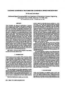
weight estimation error (MSE)

First, the parameters t0 and ∆t of Sigma-Pi should be chosen. During this stage, the segment length is fixed to 2000ms, the value of t0 varies from 100ms to 1000ms at 100ms intervals, and ∆t varies from 50ms to 300ms at 50ms intervals. The tests are carried out for all combinations of t0 and ∆t. Results show that when t0=500ms and ∆t=150ms, the performance is the best. These two parameters are then taken as the basic parameters for the following experiments. 0.005 Test set Training set

0.004 0.003 0.002 0.001 0.000

0

1000

2000 3000 4000 segment length (ms)

5000

Fig. 4. Weight estimation error on training and test set depending on segment length

The performance of weight estimation is also affected by the segment length. The weight estimation errors depending on different segment length are measured by mean square error (MSE) between the estimated weight value λ’A and the actual one λA, where l is the number of weight values in the data set: MSE =

1 l

∑ ( λ Ai − λ Ai' ) l

2

.

(3)

i =1

The results are illustrated in figure 4, which show that MSE decreases with the segment length getting longer either on training or test set. When the segment length is greater than 1500ms, MSE decreases little. The segment length of 1500ms is chosen for the following experiment.

5.3 Speaker Identification Results We conduct the speaker identification experiments with fixed noise and random varying noise conditions (with mean acoustic SNR varies from 30dB to 0dB at 10dB intervals) through the whole sentence. Two different weight estimation methods are tested: (1) fixed weight, the fusion weight remains fixed for the test set after trained, as the tradition way mentioned in [2-4]; (2) our proposed method, the estimated weight changes automatically according to the acoustic noise conditions. The experimental results on our homegrown Chinese database are summarized in table 1. The experiments are also conducted on the CMU English database to check the validation of the proposed method. The results are summarized in table 2. It can be seen that the method proposed in this paper improves the accuracies of speaker identification at different acoustic SNR levels when the noise varies dynamically comparing to the traditional fixed weight method. When the acoustic noise changes, that is to say the noise condition for the test set varies and does not match with the training set, the performance degrades dramatically for the traditional fixed weight method, while the performance differences are not significant for the proposed method in this paper. It indicates that our proposed method can predict the fusion weight well under dynamically varying acoustic noise conditions, and can improve the performance of the audio-visual bimodal speaker identification. Table 1. Accuracies of speaker identification on our own database with different fusion weight estimation method

mean SNR 30dB 20dB 10dB 0dB fixed varying fixed varying fixed varying fixed varying fixed weight 100% 98% 91% 85% 79% 72% 76% 70% proposed method 100% 100% 91% 90% 80% 78% 77% 75% Table 2. Accuracies of speaker identification on CMU database with different fusion weight estimation method

mean SNR 30dB 20dB 10dB 0dB fixed varying fixed varying fixed varying fixed varying fixed weight 100% 99% 92% 86% 81% 77% 77% 73% proposed method 100% 100% 93% 92% 81% 81% 79% 78%

6 Conclusions We investigate a fusion weights estimation method of multi-level hybrid fusion for audio-visual speaker identification by means of support vector regression (SVR). The proposed method estimates the fusion weights directly from the audio features. In the method, Sigma-Pi network re-sampling is introduced to reduce the dimensions of the audio features. The experiments show that the method improves the speaker identification performance at different acoustic SNR levels under varying acoustic noise

conditions, which indicates that the proposed method can predict the fusion weight well under such circumstances.

7 Acknowledgments This work is supported by the joint research fund of NSFC-RGC (National Natural Science Foundation of China - Research Grant Council of Hong Kong) under grant No. 60418012 and N-CUHK417/04.

References 1. Senior, A., Neti, C., Maison, B.: On the use of visual information for improving audio-based speaker recognition. In: Proc. Audio-visual Speech Processing Conf. (1999) 108–111 2. Nefian, A.V., Liang, L.H., Fu, T.Y., Liu, X.X.: A Bayesian approach to audio-visual speaker identification. In: Proc. 4th Int. Conf. Audio- and Video-based Biometric Person Authentication, Vol. 2688 (2003) 761–769 3. Chibelushi, C.C., Deravi, F., Mason, J.S.D.: A review of speech-based bimodal recognition. IEEE Trans. Multimedia 4 (2002) 23–37 4. Dupont, S., Luettin, J.: Audio-visual speech modeling for continuous speech recognition. IEEE Trans. Multimedia 2 (2000) 141–151 5. Wu, Z.Y., Cai, L.H., Meng, M.H.: Multi-level fusion of audio and visual features for speaker identification. In: Proc. Int. Conf. Biometrics, LNCS 3832 (2006) 493–499 6. Scholkopf, B., Smola, A.J., Williamson, R.C., Bartlett, P.L.: New support vector algorithms. Neural Computation 12 (2000) 1083–1121 7. Gramß, T., Strube, H.W.: Recognition of isolated words based on psychoacoustics and neurobiology. Speech Communication 9 (1990) 35–40 8. Chen, T.: Audiovisual speech processing. IEEE Trans. Signal Processing 18 (2001) 9–21 9. Bilmes, J., Zweig, G.: The graphical models toolkit: An open source software system for speech and time-series processing. In: Proc. Int. Conf. Acoustic Speech and Signal Processing. (2002) 3916–3919