Weight functions impact on LSA performance Preslav Nakov, Antonia Popova, Plamen Mateev Faculty of Mathematics and Informatics, Sofia University “St. Kliment Ohridski” 5, James Bourchier blvd., Sofia, Bulgaria
[email protected],
[email protected],
[email protected]
Abstract This paper presents experimental results of usage of LSA for analysis of English literature texts. Several preliminary transformations of the frequency text-document matrix with different weight functions are tested on the basis of control subsets. Additional clustering based on correlation matrix is applied in order to reveal the latent structure. The algorithm creates a shaded form matrix via singular values and vectors. The results are interpreted as a quality of the transformations and compared to the control set tests.
1. Introduction The Latent Semantic Analysis (LSA) is a powerful statistical technique for indexing, retrieval and analysis of textual information used in different fields of the human cognition during the last decade. Although it is a comparatively old and well-studied technique, there are several important problems that still remain unsolved. The effective usage of LSA is a process of very sophisticated tuning and can be viewed as kind of art. The main factors that influence the results quality obtained by LSA are the following: • Pre-processing (stop-words, stemming) • Frequency matrix transformations • Choice of dimensionality • Choice of similarity measure The purpose of this paper is to study the impact of the frequency matrix transformations in isolation while keeping the other parameters fixed. LSA is fully automatic and does not use any preliminary constructed dictionaries, semantic networks, knowledge bases, conceptual hierarchies, grammatical, morphological or syntactic analysers, etc. The general idea is that there exists a set of latent dependencies between the words and their contexts (phrases, paragraphs and texts). They both are represented in the same semantic space. The identification and proper treatment of the latent
dependency permits LSA to deal successfully with the synonymy and partially with the polysemy, which are the major problems in the word-based approaches. LSA is a two-stage process and includes learning and analysis of the indexed data. During the learning phase LSA performs an automatic document indexing. The process starts with construction of a matrix X whose columns are associated with documents, and whose rows with terms (words or key-phrases). Its cell (i,j) contains the frequency (possibly transformed using a weight function) of term i in document j. The matrix X is then submitted to singular value decomposition (SVD) which results three matrices T, D (orthonormal) and S (diagonal), such that X=TSDt. Some of the rows and columns of T, S and D are removed, which is supposed to remove the unnecessary noise. This results in compression of the source space in much smaller one where there are only a limited number of significant factors (usually between 50 and 400). The newly obtained matrix X′=T′S′Dt′ is the least squares best-fit approximation of X. Thus, a vector (column in the D′S′ matrix) of reduced dimensionality is associated with each term or document. It is possible to perform a sophisticated SVD, which speeds up the process by directly finding the truncated matrices T′, S′ and D′ (Berry et al. 93). The second phase is the analysis. Most often this includes a study of the proximity between a couple of documents, a couple of words or between a word and a document. A simple mathematical transformation using the singular values and vectors from the training phase permits to obtain the vector for a non-indexed text. This permits the design of a LSA based natural language search engine. The proximity degree between two documents can be calculated as a dot product between their normalised LSA vectors. The usage of other measures is also possible, e.g.: Euclidean and Manhattan distances, Minkowski measures, Pearson’s correlation
coefficient etc. (Deerwester et al. 90; Laudauer et. al. 98; Nakov 00).
The trivial local weight function is equal to the term frequency tf(i,j) of term i in document j. The term frequency in logarithmic scale is used to diminish the large numbers. Extreme suppression gives the binary weight function — it is equal to 1 when tf(i,j)>0 and 0, otherwise. We use the first two local weight functions LWF = 0: term-frequency L(i,j) = tf(i,j), LWF = 1: logarithm L(i,j) = log(tf(i,j)+1). Here and later the base of the logarithmic function is assumed to be equal to 2.
df(i) for the number of documents in which term i appears, and ndocs for the number of documents or text fragments in the set of consideration. The third global weight function (GWF=2), known as GfIdf, is the ratio of the global frequency of a term and the number of documents in which it appears: G(i) = gf(i)/df(i). By combining GWF=2 with LWF=0 we get the conditional probability p(i,j)=tf(i,j)/gf(i) of the document j under condition that the term i appears, multiplied by df(i). The last number is proportional (multiplied by ndocs) to the probability of appearance of the term under the presupposition that the terms are chosen equally likely. The combination GWF=2 with LWF=1 has not probability interpretations. The global weight function (GWF=3) named Idf is usually defined by: G(i) = 1+ log (ndocs/df(i)). It may be interpreted as the quantity of information of appearance of the term i plus 1. Note that the realisation of the event A with probability P(A) may be declared (approximately) by –logP(A) bits of information. The global weight function referred to as entropy (GWF=5) is given by G(i)= 1+{Σj p(i,j) log p(i,j)}/ log ndocs. Actually, this equation represents some entropy ratio, i.e. G(i)= 1– H(d|i)/H(d), where H(d) is the entropy of the distribution (uniform) of the documents and H(d|i) is the entropy of the conditional distribution given that the term i appeared. The last tested global function (GWF=4) is the real entropy of the conditional distribution: G(i) = H(d|i) = – Σj p(i,j) log p(i,j).
2.2. Global weight functions (GWF)
3. Related work
The first global weight function (GWF=0) is the trivial G(i)=1. Combined with the trivial local weight function it gives as a result no transformation. The second one, cited as normal (GWF=1) represents normalisation of the rows, i.e. the terms' local weights: G(i) = 1/sqrt(Σj L(i,j)2). In the definition of the rest global weight functions the following notation is used: gf(i) for the global frequency of term i;
The weight functions considered follow to some extent the classic weightings considered by previous researchers. (Dumais 91; Jones 72) propose three local weightings: term frequency, logarithm and binary, and 4 global weightings: Normal, GfIdf, Idf and Entropy. We skipped the binary weighting as it is proved to be not beneficial and added the classical entropy to the potentially useful global weightings. Although there are 4*5=20 different combinations (we added the possibility of no-weighting) Dumais
2. Weight functions The matrix X is usually transformed using the socalled weight functions. Thus, the cell (i,j) contents should be a better approximation of the interrelations between terms and documents: columns are associated with documents and the rows — with terms (words or key-phrases). It is convenient to express the transformation as a product of two numbers — local and global weight functions (Witter 97; Dumais 91): a (i,j) = L(i,j)*G(i). The local weight function L(i,j) presents the weight of term i in document j. The global weight function G(i) is used to express the weight of the term i across the entire document set. Two different local functions and six global functions were involved in our considerations. The twelve combinations are noted by LWF*GWF, where LWF = 0 or 1 and represents the number of the local weight function and GWF = 0,1,2,3,4 or 5 and represents the global one.
2.1. Local weight functions (LWF)
investigated only 6 combinations: tf-raw, tf-normal, tf-gfidf, tf-idf, tf-entropy and log-entropy. Five different test collections have been considered and the weightings have been evaluated (ADI, MED, CISI, CRAN and TIME) in terms of average precision on several fixed recall levels. She obtained decrease in performance for both tf-normal and tfgfidf over the base-line tf-raw, while the quality increased for tf-idf, tf-entropy and log-entropy.
4. Experiments The experiments were performed on two English literature texts we collected on the Web from the Gutenberg Project (http://sailor.gutenberg.org): The Adventures of Sherlock Holmes by Arthur Conan Doyle and Huckleberry Finn by Mark Twain. We have chosen these two texts since they are of almost equal sizes of approximately 500 KB. The file contents were carefully investigated and all HTML tags and Gutenberg project headers were discarded. Since LSA tries to capture the mutual dependences between the words and their contexts it is of crucial importance to provide contexts of reasonable sizes. Usually, when indexing small documents they are passed as they are, since it is best to work on the whole document. It is clearly not the case here and we split both documents into chunks of size of approximately 2 KB (we took care not to split sentences). The size of 2 KB was chosen after some experiments with different splittings as the most appropriate for detecting the differences between the different weight functions. Thus, we obtained 541 chunks of 2 KB each: 272 for The Adventures of Sherlock Holmes and 269 for Huckleberry Finn by Mark Twain. We kept 10% of the set apart to be used later as a training set (54 chunks: 27 chunks from each of the oeuvres). 250 200 150 100
199
188
177
166
155
144
133
122
111
89
78
67
56
45
34
23
1
12
0
100
50
Figure 1: Singular values
The stop-words from a pre-selected list (e.g. of, the, from, for) and the words met in just one document
were removed since they cannot contribute to the proximity. We thus reduced the total different nonstop word forms considered from 10316 to 5534. In order to keep the results clean no word stemming was performed nor complex terminology couples were used since the author could prefer one word form to another. A crucial moment when using LSA is the correct choice of dimensionality. Figure 1 shows the top 200 singular values sorted in descending order. The curve goes straight down and then flattens. We have to cut the singular values around the place where the curve behaviour changes. If we cut further we lose important information and if we keep more values we start modelling the noise. Figure 1 shows that for our case this value is somewhere between 10 and 20. 0*0 0*1 0*2
0*3 0*4 0*5 1*0 1*1 1*2
1*3 1*4 1*5
129.70 8.05 480.03 441.63 22.32 44.72 100.74 6.48 185.57 324.24 16.75 178.18 82.97 4.23 236.89 349.90 18.17 30.72 48.93 3.27 130.08 202.85 10.49 82.39 61.78 2.81 130.93 226.24 13.43 20.32 32.11 1.89 83.48 162.67 8.72 49.45 43.49 2.70 115.50 164.63 11.88 15.37 29.16 1.68 56.70 128.36 7.22 48.49 38.27 2.34 96.16 157.88 10.67 14.63 26.11 1.64 50.64 120.16 7.20 43.28 37.21 2.25 83.98 138.06 10.49 13.34 24.69 1.56 45.20 115.20 6.88 41.46 35.77 2.20 77.21 135.89 10.29 13.09 23.33 1.54 44.15 107.06 6.85 39.71 32.31 2.04 70.53 134.32 9.37 12.91 22.82 1.49 39.81 104.74 6.71 38.60 32.09 2.01 67.96 133.27 9.19 12.76 22.31 1.47 38.50 104.33 6.70 37.31 31.52 2.00 65.06 131.86 9.07 12.56 21.87 1.45 36.59 103.45 6.65 36.71 30.48 1.97 62.10 129.74 9.05 12.41 21.59 1.42 35.06 100.76 6.59 36.21 29.84 1.91 54.86 129.27 8.98 12.31 20.99 1.39 34.02 100.12 6.45 35.80 29.46 1.86 53.42 126.14 8.95 12.16 20.51 1.37 33.46 99.11
6.42 34.44
28.36 1.82 50.12 125.62 8.65 12.10 20.34 1.35 33.06 98.79
6.40 34.39
27.72 1.77 49.07 122.06 8.63 11.78 20.06 1.35 32.19 97.60
6.35 33.64
Table 1: Singular values for the 12 weight functions
When different weight functions are applied we obtain very different singular values but the corresponding curve has similar behaviour. After a careful investigation we decided to use the dimensionality of 15 for all the weight functions in order to obtain comparable results. Table 1 shows the top 15 singular values in descending order when the different weight functions were applied. As was mentioned above we used 2x6=12 different weight functions. For each of these cases we calculated the dot products between all document couples. Thus we obtained correlation matrices corresponding to the documents (487x487). Figures 2 and 3 show the correlation matrices maps in 5 different colours for the five correlation intervals: 87,5-100%, black colour; 75-87,5%, dark grey; 62,575%, grey; 50-62,5%, light grey; 0-50%, white. The
chunks are arranged in a way that these from The Adventures of Sherlock Holmes come first and just then come the ones from Huckleberry Finn without any mixture. There are always several ways to express the same thought and the authors are forced to choose between different syntactic constructions, synonyms and terminology according to the intended audience and the impact the text must produce. Furnas, Landauer, Gomez and Dumais have shown (Furnas et. al. 86) that people use the same words to describe the same subject only 10-20% of the time.
appear etc. (Biber 89; Karlgen 94)). Recent experiments show that the application of LSA is another way to distinguish the texts created by different authors. (Nakov 01) A well-known property of LSA is that it maps the semantically related texts next to each other in the vector space. Thus, in our particular case the chunks from the same oeuvre tend to be more similar to each other than those coming from different oeuvres. Looking at figures 2 and 3 we can see two dark rectangles of almost equal size showing the higher proximity between the chunks from the same oeuvre.
Figure 2: Correlation matrices maps. LWF=0
Authors make their choices according to both the specific text intention and their own subjective preferences. They (denoted as style) are consistent (along the text or all the author’s oeuvres) and easy to discover for humans but very hard to describe and measure. Researchers in statistical stylistics have concentrated at word-based statistics (word length, word length distribution, long words count, type/token ratios (Losee 96)), text-based statistics (sentence length, clause complexity (Klare 63; Lorge 59)) and statistics based on specific items (pronouns counts, presence/absence of contractions/amplifiers, relative frequency of specific verbs: e.g. seem,
Figure 3: Correlation matrices maps. LWF=1
We exploited this feature to test the quality of the different weight functions in the following manner. Each of the test chunks is projected in the semantic space of the 487 chunks and its cosine with all of them is calculated. These cosines are then sorted in descending order and the precision at the levels of 10, 20, 30, 40, 50, 60, 70, 80, 90 and 100 is calculated. Given a specific test chunk and a fixed level we define the precision as the ratio of the chunks that share a common oeuvre with the test chunk to the number of the chunks in that level. For
example consider a test chunk from the Huckleberry Finn and let 47 among the 50 top ranked chunks are from the same oeuvre. Then the precision at 50 will be 47/50=0,94. We calculated the average precision for all the 54 test chunks as well as separately for both oeuvres (27 test chunks for each). The following tables 2,3,4 and 5 show the precision for each of the weight functions considered. We apply additional clustering based on correlation matrix in order to reveal the latent structure. The aim is to determine the natural document classes. This partition is to be used for further classification of the documents. Such problem is considered in the project DIDONA: Internet Technologies for Document Categorization, where the classes are fixed using expert opinion. (Mateev et al. 99) Level
0*0 holmes finn
0*1 AVG
holmes finn
holmes finn
Level
1*0 holmes finn
1*1 AVG
holmes finn
1*2 AVG
holmes finn
AVG
10
0.989 0.963 0.976
0.967 0.989 0.978
0.985 0.970 0.978
20
0.985 0.965 0.975
0.954 0.980 0.967
0.972 0.945 0.958
30
0.974 0.967 0.970
0.947 0.979 0.963
0.969 0.940 0.954
40
0.970 0.965 0.968
0.942 0.976 0.959
0.963 0.930 0.946
50
0.965 0.962 0.964
0.936 0.977 0.957
0.964 0.920 0.942
AVG
60
0.962 0.961 0.961
0.938 0.975 0.957
0.961 0.916 0.938
0.962 0.954 0.958
0.939 0.973 0.956
0.958 0.913 0.936
0*2 AVG
decomposed as a product of the form X=TSD. After the removal of most of the least significant singular values we obtain X′=T′S′D′. The process of cutting some of the singular values can be explained by a form of factor analysis and especially as a principal component analysis. Under the factor analysis consideration the matrix X is written in the form X = FA + U, where A is the matrix of the factor weights, F is the matrix of factor vectors and U is the errors matrix. Now coming back to SVD we obtain A=D′S′.
10
0.993 0.930 0.962
0.974 0.963 0.969
0.974 0.919 0.947
70
20
0.984 0.939 0.961
0.974 0.958 0.966
0.965 0.917 0.941
80
0.960 0.953 0.956
0.933 0.970 0.952
0.957 0.908 0.932
90
0.960 0.948 0.954
0.930 0.965 0.948
0.953 0.903 0.928
30
0.979 0.941 0.960
0.973 0.949 0.961
0.958 0.899 0.928
40
0.975 0.930 0.952
0.969 0.946 0.957
0.955 0.884 0.920
100 0.956 0.944 0.950
0.926 0.965 0.945
0.948 0.898 0.923
AVG 0.968 0.958 0.963
0.941 0.975 0.958
0.963 0.924 0.944
50
0.974 0.927 0.951
0.963 0.949 0.956
0.950 0.870 0.910
60
0.966 0.923 0.944
0.956 0.943 0.950
0.946 0.862 0.904
70
0.967 0.916 0.942
0.950 0.936 0.943
0.943 0.850 0.897
80
0.959 0.907 0.933
0.944 0.928 0.936
0.940 0.840 0.890
90
0.956 0.899 0.927
0.937 0.924 0.930
Table 4: Precision table for LWF=1, GWF=0,1,2 Level
1*3 holmes finn
0.938 0.830 0.884
1*4 AVG
holmes finn
1*5 AVG
holmes finn
AVG
100 0.950 0.895 0.922
0.933 0.918 0.926
0.937 0.819 0.878
10
0.985 0.993 0.989
1.000 0.996 0.998
0.985 0.993 0.989
AVG 0.970 0.921 0.945
0.957 0.941 0.949
0.950 0.869 0.910
20
0.980 0.989 0.984
0.997 0.989 0.993
0.982 0.993 0.987
30
0.972 0.990 0.981
0.995 0.993 0.994
0.977 0.993 0.985
40
0.971 0.990 0.981
0.994 0.988 0.991
0.975 0.992 0.983
Table 2: Precision table for LWF=0, GWF=0,1,2 Level
0*3 holmes finn
0*4 AVG
holmes finn
0*5 AVG
holmes finn
50
0.968 0.989 0.979
0.993 0.989 0.991
0.978 0.989 0.983
AVG
60
0.969 0.986 0.977
0.992 0.987 0.990
0.975 0.988 0.982
0.966 0.983 0.974
0.988 0.986 0.987
0.971 0.987 0.979
10
1.000 0.959 0.980
0.993 0.989 0.991
1.000 0.963 0.982
70
20
0.997 0.952 0.974
0.995 0.982 0.988
0.998 0.954 0.976
80
0.964 0.981 0.972
0.986 0.984 0.985
0.970 0.986 0.978
90
0.961 0.979 0.970
0.984 0.981 0.982
0.965 0.981 0.973
30
0.996 0.943 0.970
0.991 0.970 0.981
0.998 0.951 0.974
40
0.996 0.938 0.967
0.986 0.970 0.978
0.998 0.943 0.970
100 0.957 0.977 0.967
0.982 0.979 0.980
0.964 0.978 0.971
AVG 0.969 0.986 0.977
0.991 0.987 0.989
0.974 0.988 0.981
50
0.995 0.935 0.965
0.984 0.969 0.977
0.997 0.941 0.969
60
0.994 0.935 0.964
0.985 0.969 0.977
0.995 0.937 0.966
70
0.994 0.933 0.963
0.985 0.967 0.976
0.993 0.932 0.962
80
0.993 0.928 0.960
0.984 0.966 0.975
0.992 0.930 0.961
90
0.990 0.923 0.957
0.983 0.965 0.974
0.992 0.926 0.959
100 0.989 0.919 0.954
0.983 0.963 0.973
0.990 0.922 0.956
AVG 0.994 0.936 0.965
0.987 0.971 0.979
0.995 0.940 0.967
Table 3: Precision table for LWF=0, GWF=3,4,5
The partitioning algorithm creates a shaded-form matrix by means of singular values and vectors. As was mentioned in section 2 the initial matrix X is
Table 5: Precision table for LWF=1, GWF=3,4,5
We apply a rearrangement algorithm on A. We sort the columns in descending order by the dispersion explained by the factors. Then we arrange the rows in a way that for each subsequent factor the weights greater than 0.5 are arranged in descending order. After the rearrangement we compute AAt, which gives X′tX′. This way the documents are arranged in a way that the documents with higher proximity in
LSA sense are grouped on the main diagonal in subsequent clusters.
and the formal evaluation in terms of precision from tables 2,3,4 and 5.
5. Discussion
Figure 4: Rearranged matrix. LWF=1, GWF=3
Figure 5: Rearranged matrix. LWF=1, GWF=4
Figures 4 and 5 show the results of the application of the algorithm for the weightings 1*3 and 1*4. We can see two major groups of chunks on the main diagonal, which is natural: we have two texts and thus two groups of chunks. Several smaller groups of chunks that are much dissimilar from the other ones following them are bounded. The bigger and clearer clusters formed by 1*4 show that it is a better weighting scheme. This is consistent with both the correlation matrices from figures 2 and 3
The results clearly show that both local and global weight functions are important and influence the results. On the other hand looking globally they seem to be independent from each other to some extent. Consider tables 2 and 3 which contain the precision for LWF=0. If we arrange (in descending order) the GWF according to the average precision we get the following ordering: 4,5,3,1,0,2. We obtain exactly the same ordering for LWF=1 (tables 4 and 5). Thus, we conclude that this ordering is the one that gives the true importance of the global weight functions. Although, looking from The Adventures of Sherlock Holmes point of view we get a bit different orderings: 5,3,4,0,1,2 (LWF=0) and 4,5,3,0,2,1 (LWF=1). For Huckleberry Finn we have the orderings 4,1,5,3,0,2 (LWF=0) and 5,4,3,1,0,2 (LWF=1). This means that LWF and GWF are dependent from each other as well as on the particular text they are applied on. If we fix the GWF and look at the results for LWF globally we see that for all the six values of GWF the application of LWF=1 (logarithm) is always beneficial compared to LWF=0 and results in higher average precision. The same applies at text level for Huckleberry Finn. Although, looking at The Adventures of Sherlock Holmes we get just the reverse: the application of logarithm (LWF=1) consistently harms the precision regardless of the GWF applied. While the application of logarithm as a LWF seems to give inconsistent results at text level we can nevertheless consider it is beneficial because of its superior performance looking globally. Thus, while it harms the performance for one of the texts it is much more beneficial for the other text. Looking at GWF we discover two groups of functions: 0,1,2 and 3,4,5. Looking at tables 2,3,4 and 5 we can conclude the first group results in lower precision regardless of the text and the LWF applied. Surprisingly, the classical entropy function 4 demonstrates consistently superior performance to function 5 although the latter one is usually preferred when using LSA (Witter 97; Jiang 97; Dumais 93,94,95). This should be tested on different corpora and possibly by using different evaluation
techniques. Looking at figures 2 and 3 we can see that although the rectangles for the two texts are much clear for function 4 than for 5 they contain a higher degree of noise outside. The results obtained are consistent with previous research in the field. As was mentioned above (Dumais 91) evaluated on 5 different text collections some of the functions we consider here: 0*0, 0*1, 0*2, 0*3, 0*5 and 1*5. Her study differs from ours not only due to the larger number of function combinations we consider and the different text collections used but also on the way the performance is evaluated: We are interested in text categorisation while her primary goal was information retrieval. She accepted 0*0 as the base-line weighting and obtained decrease in performance for 0*1 (–11%) and 0*2 (–7%), and increase — for 0*3 (+27%), 0*4 (+30%) and 1*5 (+40%). Thus, her ordering is: 0*1 < 0*2 < 0*0< 0*3 < 0*4 < 1*5. Our AVG ordering follows the pattern only partially: 0*2 < 0*0 < 0*1 < 0*3 < 0*4 < 1*5. Looking at Holmes we see: 0*2 < 0*1 < 0*0 < 0*5 < 0*4 < 1*5, and for Finn we have: 0*2 < 0*0 < 0*3 < 1*5 < 0*1 < 0*5. While this reordering may seem quite different most of the numbers behind are very next to each other. It is important to stress that her data is obtained as the average of 5 different text collections each of which has its own ordering that sometimes differs from the overall results.
6. Future work Additional experiments on new text collections with new authors (including languages different from English) have to be performed in order to justify the results obtained and to better understand the factors influencing the text proximity when using LSA. There is some place for tuning both the sorting and the clustering algorithms. Different combinations of more authors and oeuvres (including more than one oeuvre per author) are to be considered. Some new local and global weight functions as well as new evaluation methods are under consideration for future experiments.
References:
(Deerwester et al. 90) Deerwester S., Dumais S., Furnas G., Laundauer T., Harshman R. Indexing by Latent Semantic Analysis. Journal of the American Society for Information Sciences, 41. 1990. (Dumais 91) Dumais S. Improving the retrieval of information from external sources. Behavior Research Methods, Instruments, & Computers, 23(2):229-236.1991. (Dumais 93) Dumais, S. LSI meets TREC: A status report. In: D. Harman (Ed.), The First Text REtrieval Conference (TREC1). National Institute of Standards and Technology Special Publication 500-207, pp. 137-152. 1993. (Dumais 94) Dumais, S. Latent Semantic Indexing (LSI) and TREC-2. In: D. Harman (Ed.), The Second Text REtrieval Conference (TREC2), National Institute of Standards and Technology Special Publication 500-215 , pp. 105-116. 1994. (Dumais 95) Dumais, S. Using LSI for information filtering: TREC-3 experiments. In: D. Harman (Ed.), The Third Text REtrieval Conference (TREC3) National Institute of Standards and Technology Special Publication , in press 1995. (Furnas et. al. 86) Furnas G., Landauer T., Gomez L. and Dumais T. Statistical semantics: Analysis of the Potential Performance of Keyword Information Systems. Bell Syst.Tech.J., 62, Number 6, pp. 1753-1806, 1986. (Harman 91) Harman, D. How effective is suffixing? In Journal of The American Society of Information Science. Vol. 42, No 1. 1991. (Jiang 97) Jiang, J. Using Latent Semantic Indexing for Data Mining. Department of Computer Science, University of Tennessee. 1997. (Jones 72) Jones, K. Sparck. A statistical interpretation of term specificity and its applications in retrieval, J. Documentation, 28, pp. 11-21. 1972. (Karlgen 94) Karlgen J., Douglas C. Recognizing Text Genres with Simple metrics Using Discriminant Analysis. Proceedings of COLING 94, Kyoto, pp. 1071-1075. 1994. (Klare 63) Klare G.The Measurement of Readability. Ames: Iowa University Press. 1963. (Laudauer et. al. 98) T., Foltz P., Laham D. Introduction to Latent Semantic Analysis. Discourse Processes, 25. 1998. (Lorge 59) Lorge I. The Lorge Formula for Estimating Difficulty of Reading Materials. New York: Teachers College Press, Columbia University, 1959. (Losee 96) Losee R. Text Windows and Phrases Differing by discipline, Location in Document, and Syntactic Structure.Information Processing & Management 32(Nov): 747-67. 1996 (Nakov 00) Nakov P. Getting Better Results with Latent Semantic Indexing. In Proceedings of the Students Presentations at ESSLLI2000, Birmingham, UK. 2000. (Nakov 01) Nakov P. Latent Semantic Analysis for Bulgarian literature. In Proceedings of Spring Conference of Bulgarian Mathematicians Union. Borovetz. 2001. (Mateev et al. 99) Mateev P., Nikolova N., Angelova G., Text Categorization in an Internet Application for Document Management, IJCAI, Stockholm.1999. (Salton 71) Salton, G., The SMART Retrieval System - Experiment in Automatic Document Processing, Prentice-Hall, Englewood Cliffs, New Jersey. 1971.
(Berry et al. 93) Berry M., Do T., O'Brien G., Krishna V., and Sowmini Varadhan. SVDPACKC Version 1.0. User's Guide. 1993.
(Witter 97) Witter, D. I. Downdating the Latent Semantic Indexing Model for Information Retrieval. Department of Computer Science, University of Tennessee. 1997.
(Biber 89) Biber D. A typology of English Texts. Linguistics, 27, pp. 343. 1989.
Gutenberg Project. http://sailor.gutenberg.org LSA. 1990-2001, see http://lsa.colorado.edu