Weighted Set-Based String Similarity Marios Hadjieleftheriou AT&T Labs–Research
[email protected]
Divesh Srivastava AT&T Labs–Research
[email protected]
Abstract Consider a universe of tokens, each of which is associated with a weight, and a database consisting of strings that can be represented as subsets of these tokens. Given a query string, also represented as a set of tokens, a weighted string similarity query identifies all strings in the database whose similarity to the query is larger than a user specified threshold. Weighted string similarity queries are useful in applications like data cleaning and integration for finding approximate matches in the presence of typographical mistakes, multiple formatting conventions, data transformation errors, etc. We show that this problem has semantic properties that can be exploited to design index structures that support very efficient algorithms for query answering.
1
Introduction
Arguably, one of the most important primitive data types in modern data processing is strings. Short strings comprise the largest percentage of data in relational database systems, long strings are used to represent protein and DNA sequences in biological applications, as well as HTML and XML documents on the web. Searching through string datasets is a fundamental operation in almost every application domain, for example SQL query processing, information retrieval, genome research, product search in eCommerce applications, and local business search on online maps. Hence, a plethora of specialized indexes, algorithms, and techniques have been developed for searching through strings. Due to the complexity of collecting, storing and managing strings, string datasets almost always contain representational inconsistencies due to typographical mistakes, multiple formatting conventions, data transformation errors, etc. Most importantly, string keyword queries more often than not contain errors as well. Even though exact string matching has been studied extensively in the past and a variety of efficient string searching algorithms have been developed, it is clear that approximate string matching (based on some notion of string similarity) is fundamental for retrieving the most relevant results for a given query, and ultimately improving user satisfaction. For that purpose, various string similarity functions have been proposed in the literature. This article discusses indexing techniques and algorithms based on inverted indexes and a variety of weighted set-based string similarity functions, that can be used for efficiently answering all-match selection queries, i.e., queries which ask for all data strings whose similarity with the query string is larger than a user specified threshold.
Copyright 2010 IEEE. Personal use of this material is permitted. However, permission to reprint/republish this material for advertising or promotional purposes or for creating new collective works for resale or redistribution to servers or lists, or to reuse any copyrighted component of this work in other works must be obtained from the IEEE. Bulletin of the IEEE Computer Society Technical Committee on Data Engineering
1
2
Set-Based Similarity
Set-based similarity decomposes strings into sets of tokens (such as words or n-grams) using a variety of tokenization methods and evaluates similarity of strings with respect to the similarity of their sets. A variety of set similarity functions can be used for this purpose, all of which have a similar flavor: each set element (or token) is assigned a weight and the similarity between the sets is computed as a weighted function of the tokens in each of the sets and in their intersection. The application characteristics heavily influence the tokens to extract, the token weights, and the similarity function used.
2.1
Similarity Functions
Strings are modeled as sets of tokens from a known token set Λ. Let s = {a1 , a2 , . . . , an }, ai ∈ Λ be a string consisting of n tokens. Let W : Λ → R+ be a function that assigns a positive real weight value to each token. A simple function to evaluate the similarity between two strings is the weighted intersection of their token sets. Definition 1 (Weighted Intersection on Sets): Let s = {a1 , . . . , an }, ∑ r = {b1 , . . . , bm }, ai , bi ∈ Λ be two sets of tokens. The weighted intersection of s and r is defined as I(s, r) = a∈s∩r W (a). The definition above does not take into account the weight or number of tokens that the two strings do not have in common. In some applications, the strings are required to have similar lengths (i.e., similar number of tokens or similar total token weight). One could use various forms of normalization to address this issue. Definition 2 (Normalized Weighted Intersection, Jaccard Similarity, Dice Similarity, ∑ Cosine Similarity): Let s = {a1 , . . . , an }, r√=∑{b1 , . . . , bm }, ai , bi ∈ Λ be two sets of tokens. Let ∥s∥1 = ni=1 W (ai ) (i.e., the L1 n 2 norm), and ∥s∥2 = i=1 W (ai ) (i.e., the L2 -norm). ∥s∩r∥1 The normalized weighted intersection of s and r is defined as N (s, r) = max(∥s∥ . 1 ,∥r∥1 ) ∥s∩r∥1 ∥s|1 +|r|1 −|s∩r∥1 . 2∥s∩r∥1 defined as mathcalD(s, r) = ∥s∥ . 1 +∥r∥1 [∥s∩r∥2 ]2 is defined as: C(s, r) = ∥s∥2 ∗∥r∥2 .
The Jaccard similarity of s and r is defined as J (s, r) = The Dice similarity of s and r is The Cosine similarity of s and r
∥s∩r∥1 ∥s∪r∥1
=
Clearly, Normalized Weighted Intersection, Jaccard, Dice and Cosine similarity are strongly related in a sense that they normalize the similarity with respect to the weights of the token sets, and result in a similarity value between 0 and 1. The similarity is minimized (i.e., equal to 0) only if the two sets share no tokens in common, and is maximized (i.e., equal to one) only if the two sets are the same. In general, the larger the weight of the tokens that the two strings do not have in common, the smaller is their similarity. Which function works better depends heavily on application and data characteristics.
2.2
Token Weights
An important consideration for weighted similarity functions is the token weighting scheme used. The simplest weighting scheme is to use unit weights for all tokens. A more meaningful weighting scheme though, should assign larger weights to tokens that carry more information content. As usual, the information content of a token is application and data dependent. For example, a specific sequence of phonemes might be very rare in the English language but a common sequence in Greek. A commonly used weighting scheme for text processing is based on inverse document frequency weights. Definition 3 (Inverse Document Frequency Weight): Consider a set of strings D and a universe of tokens Λ. Let df (a), a ∈ Λ be the number of strings s ∈ D that have at least one occurrence of a. The inverse document frequency weight of a is defined as idf (a) = log(1 + df|D| (a) ). 2
String s1 s2 s3 s4 s5
Children’s One Feed International UNICEF
Tokens Food Fund Laptop per the Children Children’s Found
Child
Token child food found fund international one laptop unicef
String Identifiers s1 , s2 , s3 , s4 s1 , s3 s4 s1 s4 s2 s2 s5
Table 1: (a) A collection of strings represented as sets of tokens. (b) An inverted representation of these sets of tokens. It is assumed that common stop words and special characters have been removed, stemming of words has occurred, and all tokens have been converted to lowercase. Alternative definitions of idf weights are also possible. Nevertheless, they all have a similar flavor. The idf weight is related to the probability that a given token a appears in a random string s ∈ D. Frequent tokens have a high probability of appearing in many strings, hence they are assigned small weights. Infrequent tokens have a small probability of appearing in any string, hence they are assigned large weights. The intuition is that two strings that share a few infrequent tokens must have a high similarity.
2.3 Selection Queries We consider all-match selection queries, which return all data strings whose similarity with the query string is larger than a user specified threshold. Definition 4 (All-Match Selection Query): Given a string similarity function S, a set of strings D, a query string q, and a positive threshold τ , the result of an all-match selection query is the answer set A = {s ∈ D : S(q, s) ≥ τ }.
3 Algorithms for Set-Based Similarity The brute-force approach for evaluating selection queries requires computing all pairwise similarities between the query string and the data strings, which can be expensive. A significant savings in computation cost can be achieved by using an index structure (resulting in a typical computation cost versus storage cost trade-off). All the set-based similarity functions introduced in Section 2 can be computed easily using an inverted index. First, the data strings are tokenized and an inverted index is built on the resulting tokens, one list per token; an example using word tokens is shown in Table 1. Each list element is simply a string identifier. Depending on the algorithm used to evaluate the chosen similarity function, the lists can be stored sequentially as a flat file, using a B-tree, or a hash table. They can also be sorted according to string identifiers or any other information stored in the lists (e.g., the Lp -norm of the strings) as will become clear shortly. All-match selection queries can be answered quite efficiently using an inverted index. Recall that an allmatch selection query retrieves all data strings whose similarity with the query exceeds a query threshold τ . To answer the query, first the query string is tokenized using exactly the same tokenization scheme that was used for the data strings. The data strings satisfying the similarity threshold need to have at least one token in common with the query, hence only the token lists corresponding to query tokens need to be involved in the search. This results in significant pruning compared to the brute-force approach.
3
3.1
Sorting in String Identifier Order
Let q = {q1 , . . . , qn } be a query string and Lq = {l1 , . . . , ln } be the n lists corresponding to the query tokens. By construction, each list li contains all string identifiers of strings s ∈ D s.t. qi ∈ s. The simplest algorithm for evaluating the exact similarity between the query and all the strings in Lq is to perform a multiway merge on the string identifiers over the lists to compute all intersections q ∩ s. This will directly yield the weighted intersection similarity. Clearly, the multiway merge computation can be performed very efficiently if the lists are already sorted in increasing order of string identifiers. However, the algorithm has to exhaustively scan all lists in Lq in order to identify all strings with similarity exceeding threshold τ . Computing Normalized Weighed Intersection is also straightforward, provided that the L1 -norm of each data string is stored in the token lists. Hence, the lists store tuples (string-identifier, L1 -norm). Once again, if lists are sorted in increasing order of string identifiers, a multiway merge algorithm can evaluate the normalized weighted intersection between the query and all relevant strings very efficiently. Similar arguments hold for Jaccard, Dice and Cosine similarity.
3.2
Sorting in Lp -norm Order
The multiway merge algorithm has to exhaustively scan all the lists in Lq in order to compute the similarity score of every data string and determine whether the similarity exceeds threshold τ . For Normalized Weighed Intersection similarity we make the following observation: Lemma 5 (Normalized Weighted Intersection L1 -norm Filter): Given sets s, r and Normalized Weighted Intersection threshold τ ∈ (0, 1] the following holds: N (s, r) ≥ τ ⇔ τ ∥r∥1 ≤ ∥s∥1 ≤
∥r∥1 . τ
Essentially, we can use the L1 -norm filter to prune strings appearing in any list in Lq without the need to compute the actual similarity with the query. For that purpose, we sort token lists in increasing order of the L1 -norms of strings, rather than in string identifier order. Using Lemma 5, we can directly skip over all candidate strings with L1 -norm ∥s∥1 < τ ∥q∥1 (where ∥q∥1 is the L1 -norm of the query) and stop scanning a 1 list whenever we encounter the first candidate string with L1 -norm ∥s∥1 > ∥q∥ τ . Given that the lists are not sorted in increasing string identifier order, there are two options available: The first is to sort the strings within the appropriate norm intervals in string identifier order and perform the multiway merge in main memory. The second is to use classic threshold based algorithms to compute the similarity of each string to the query string. Threshold algorithms utilize special terminating conditions that enable processing to stop before exhaustively scanning all token lists. This is easy to show if the similarity function is a monotone aggregate function. W (qi ) Let wi (s, q) = max(∥s∥ be the partial similarity of data string s and query token qi . Then, N (s, q) = 1 ,∥q∥1 ) ∑ ′ qi ∈s∩q wi (s, q). It can be shown that N (s, q) is a monotone aggregate function, i.e., N (s, q) ≤ N (s , q) if ∀i ∈ [1, n] : wi (s, q) ≤ wi (s′ , q). There are three threshold algorithm flavors. The first scans lists sequentially and in a round robin fashion and computes the similarity of strings incrementally. The second uses random accesses to compute similarity aggressively every time a new string identifier is encountered in one of the lists. The third uses combination strategies of both sequential and random accesses. Since the sequential round robin algorithm computes similarity incrementally, it has to temporarily store in main memory information about strings whose similarity has only been partially computed. Hence, the algorithm has a high book keeping cost, given that the candidate set needs to be maintained as a hash table organized by string identifiers. The aggressive random access based algorithm computes the similarity of strings in one step 4
and hence does not need to store any information in main memory. Hence it has a very small book keeping cost, but on the other hand it has to perform a large number of random accesses to achieve this. This could be a drawback on traditional storage devices (like hard drives) but unimportant in modern, solid state based devices, like flash storage. Combination strategies try to strike a balance between low book keeping and a small number of random accesses. A simple round robin strategy is shown in Algorithm 3.1. Algorithm 3.1:
N R A (q, τ )
Tokenize the query: q = {q1 , . . . , qn } M is a map of (¨ s, Ns , B1 , . . . Bn ]) tuples (Bi are bits, s¨ is the string identifier) for i ← 1 to n do seek li to first element s.t. ∥s∥1 ≥ τ ∥q∥1 while not all lists li are inactive f = ∞, w = 0 for i ← 1 to n if li is inactive : Continue else (¨ s, ∥s∥1 ) ← li .next ∥q∥1 if ∥s∥ 1 > τ : Flag li as inactive and Continue f = min(f, ∥s∥1 ), w = w + W (qi ) (¨ s, Ns , B1 , . . . , Bn ) ← M.find(¨ s) for j ← 1 to n do do if lj is inactive : Bj = 1 if s¨ ∈ M if B1 = 1, . . . , Bn = 1} and Ns + W (qi ) > τ max(∥s∥1 , ∥q∥1 ) then report s¨, Ns + W (qi ) then s, Ns + W (qi ), B1 , . . . , Bn ) { else M ← (¨ M ← (¨ s , W (q ), B1 , . . . , Bn ) else i for all (¨ s , N , B , . . . , B ) ∈ M s 1 n for j ← 1 to n do if lj is inactive : Bj = 1 if B1 = 1, . . . , Bn = 1 do if Ns > τ max(∥s∥1 , ∥q∥1 ) then report s¨, Ns then else remove from M if w < τ and M is empty : Stop max(f,∥q∥1 )
The algorithm keeps a candidate set M containing tuples consisting of a string identifier, a partial similarity score, and a bit vector containing zeros for all query tokens that have not matched with the particular string identifier yet, and ones for those that a match has been found. The candidate set is organized as a hash table on string identifiers for efficiently determining whether a given string has already been encountered or not. Lemma 5 states that for each list we only need to scan elements within a narrow L1 -norm interval. We skip directly to the first element in every list with L1 -norm ∥s∥1 ≥ τ ∥q∥1 . The algorithm proceeds by reading one element per list in every iteration, from each active list. According to Lemma 5, if the next element read from list li 1 has L1 -norm larger than ∥q∥ τ the algorithm flags li as inactive. Otherwise, if the string identifier read is already contained in the candidate set M , its entry is updated to reflect the new partial similarity score. In addition, the bit vector is updated to reflect the fact that the candidate string contains the particular query token. Also, the 5
algorithm checks whether any other lists have already become inactive, which implies one of two things: If the candidate string contains the query token, then the bit vector is already set to one and the partial similarity score has been updated to reflect that fact; or the candidate string does not contain the query token, hence the bit vector can be set to one without updating the partial similarity score (essentially adding zero to the similarity score). Finally, if the bit vector is fully set and the similarity score exceeds the query threshold, the string is reported as an answer. If the new string read is not already contained in M , a new entry is created and reported as an answer or inserted in M , using reasoning similar to the previous step. After one round robin iteration, the bit vector of each candidate in the candidate set is updated, and candidates with fully set bit vectors are reported as answers or evicted from the candidate set accordingly. The algorithm can terminate early if two conditions are met. First the candidate set is empty, which means no more viable candidates whose similarity has not been completely computed yet exist. Second, the maximum possible score of a conceptual frontier string that appears at the current position in all lists cannot exceed the desired threshold. Lemma 6: Let La ⊆ Lq be the set of active lists. The terminating condition ∑ li ∈La W (qi ) f N = < τ, max(minli ∈La ∥fi ∥1 , ∥q∥1 ) does not lead to any false dismissals. It is easy to see that a tighter bound for N f exists. This can be achieved by examining the L1 -norm of all frontier elements simultaneously and is based on the observation that Observation 7: Given a string s with L1 -norm ∥s∥1 and the L1 -norms of all frontier elements ∥fi ∥1 we can immediately deduce whether s potentially appears in list li or not by a simple comparison: If ∥s∥1 < ∥fi ∥1 and s has not been encountered in list li yet, then s does not appear in li (given that lists are sorted in increasing order of L1 -norms). Let lj be a list s.t. ∥fj ∥1 = minli ∈La ∥fi ∥1 . Based on Observation 7, a conceptual string s with L1 -norm ∥s∥1 = ∥fj ∥1 can appear only in list lj . Thus Lemma 8: Let La ⊆ Lq be the set of active lists. The terminating condition ∑ lj ∈La :∥fj ∥1 ≤∥fi ∥1 W (qj ) f < τ, N = max li ∈La max(∥fi ∥1 , ∥q∥1 ) does not lead to any false dismissals. We can also use Observation 7 to improve the pruning power of the nra algorithm by computing a best-case similarity for all candidate strings before and after they have been inserted in the candidate set. Strings whose best-case similarity is below the threshold can be pruned immediately, reducing the memory requirements and the book keeping cost of the algorithm. The best-case similarity of a new candidate uses Observation 7 to identify lists that do not contain that candidate. Lemma 9: Given query q, candidate string s, and a subset of lists Lq′ ⊆ Lq potentially containing s (based on Observation 7 and the frontier elements fi ), the best-case similarity score for s is: N b (s, q) =
∥q ′ ∥1 . max(∥s∥1 , ∥q∥1 ) 6
An alternative threshold algorithm strategy is to assume that token lists are sorted in increasing L1 -norms for efficient sequential access, but that there also exists one index per token list on the string identifiers. Then, a random access algorithm can scan token lists sequentially and for every element probe the remaining lists using the string identifier index to immediately compute the exact similarity of the string. Similar terminating conditions as those used for the nra algorithm can be derived for the random access only algorithm. The last threshold based strategy is to use a combination of nra and random accesses. We run the nra algorithm as usual but after each iteration we do a linear pass over the candidate set and use random accesses to compute the exact similarity of the strings and empty the candidate set. It turns out that exactly the same length based algorithms can be used for Dice and Cosine similarity. It is easy to show that Dice similarity is a monotone aggregate function with partial similarity defined as wi (s, q) = W (qi ) ∥s∥1 +∥q∥1 . Hence, all threshold algorithms presented above can be adapted to Dice. In addition, it is easy to prove the following lemmas. Lemma 10 (Dice L1 -norm Filter): Given sets s, r and Dice similarity threshold τ ∈ (0, 1] the following holds: D(s, r) ≥ τ ⇔
2−τ τ ∥r∥1 ≤ ∥s∥1 ≤ ∥r∥1 . 2−τ τ
Lemma 11: Let La ⊆ Lq be the set of active lists. The terminating condition ∑ lj ∈La :∥fj ∥1 ≤∥fi ∥1 2W (qi ) Df = max < τ, li ∈La ∥fi ∥1 + ∥q∥1 does not lead to any false dismissals. Lemma 12: Given query q, candidate string s, and a subset of list Lq′ ⊆ Lq potentially containing s, the best-case similarity score for s is: 2∥q ′ ∥1 Db (s, q) = . ∥s∥1 + ∥q∥1 Exactly the same arguments hold for cosine similarity as well. Recall that cosine similarity is computed based on the L2 -norm of the strings. Once again, an inverted index is built where this time each list element contains tuples (string-identifier, L2 -norm). Clearly, Cosine similarity is a monotone aggregate function with W (qi )2 partial similarity wi (s, q) = ∥s∥ . An L2 -norm filter also holds. 2 ∥q∥2 Lemma 13 (Cosine similarity L2 -norm Filter): Given sets s, r and Cosine similarity threshold τ ∈ (0, 1] the following holds: ∥r∥2 C(s, r) ≥ τ ⇔ τ ∥r∥2 ≤ ∥s∥2 ≤ . τ In addition Observation 14: Given a string s with L2 -norm ∥s∥2 and the L2 -norms of all frontier elements ∥fi ∥2 we can immediately deduce whether s potentially appears in list li or not by a simple comparison: If ∥s∥2 < ∥fi ∥2 and s has not been encountered in list li yet, then s does not appear in li (given that lists are sorted in increasing order of L2 -norms). Hence Lemma 15: Let La ⊆ Lq be the set of active lists. The terminating condition ∑ 2 lj ∈La :∥fj ∥2 ≤∥fi ∥2 W (qi ) C f = max < τ, li ∈La ∥fi ∥2 ∗ ∥q∥2 does not lead to any false dismissals. 7
Lemma 16: Given query q, candidate string s, and a subset of lists Lq′ ⊆ Lq potentially containing s, the best-case similarity score for s is: [∥q ′ ∥2 ]2 C b (s, q) = . ∥s∥2 ∗ ∥q∥2 The actual algorithms in principle remain the same. Jaccard similarity presents some difficulties. Notice that Jaccard is a monotone aggregate function with W (qi ) partial similarity wi (s, q) = ∥s∪q∥ . Nevertheless, we cannot use this fact for designing termination conditions 1 for the simple reason that wi ’s cannot be evaluated on a per token list basis since ∥s ∪ q∥1 is not known in advance (knowledge of ∥s ∪ q∥1 implies knowledge of the whole string s and hence knowledge of ∥s ∩ q∥1 which is equivalent to directly computing the similarity). Recall that an alternative expression for Jaccard is ∥s∩q∥1 J (s, q) = ∥s∥1 +∥q∥ . This expression cannot be decomposed into aggregate parts on a per token basis, 1 −∥s∩q∥1 and hence is not useful either. Nevertheless, we can still prove various properties of Jaccard that enable us to use all threshold based algorithms. In particular Lemma 17 (Jaccard L1 -norm Filter): Given sets s, r and Jaccard similarity threshold τ ∈ (0, 1] the following holds: ∥r∥1 . J (s, r) ≥ τ ⇔ τ ∥r∥1 ≤ ∥s∥1 ≤ τ ∑ Lemma 18: Let La ⊆ Lq be the set of active lists. Let Ii = lj ∈La :∥fj ∥1 ≤∥fi ∥1 W (qi ). The terminating condition Ii J f = max < τ, li ∈La ∥fi ∥1 + ∥q∥1 − Ii does not lead to any false dismissals. Lemma 19: Given query q, candidate string s, and a subset of list Lq′ ⊆ Lq potentially containing s, the best-case similarity score for s is: J b (s, q) =
∥q ′ ∥1 . ∥s∥1 + ∥q∥1 − ∥q ′ ∥1
Generally speaking, comparing the threshold based algorithms with the multiway merge algorithm, the relative cost savings between sorting according to string identifiers or sorting according to the Lp -norm heavily depends on a variety of factors most important of which are: the algorithm used, the specific query (whether it contains tokens with very long lists for which the Lp -norm filtering will yield significant pruning), the overall token distribution of the data strings, the storage medium used to store the lists (e.g., disk drive, main memory, solid state drive), and the type of compression used for the lists, if any. It is important to state here that most list compression algorithms are designed for compressing string identifiers, which are natural numbers. The idea being that natural numbers in sorted order can easily be represented by delta coding. In delta coding only the first number is stored, and each consecutive number is represented by its difference with the previous number. This representation decreases the magnitude of the numbers stored (since deltas are expected to have small magnitude when the numbers are in sorted order) and enables very efficient compression. A significant issue with all normalized similarity functions is that, given arbitrary token weights, token lists have to store real valued L1 -norms (or L2 -norms for Cosine similarity). Lists containing real valued attributes cannot be compressed as efficiently as lists containing only natural numbers.
8
3.3
Processing Lists in Token Weight Order
Recall that the threshold based algorithms scan lists in a random order, e.g., in the order that tokens appear in the query string. However, the distribution of tokens in the data strings can help determine a more meaningful ordering that can yield significant performance benefits. The idea is based on the observation that the order and the strategy used to scan the lists affects the frontier elements, and hence the pruning power of subsequent steps. Consider Normalized Weighted Intersection first. Let the lists in Lq be sorted according to their respective token weights, from heaviest to lightest. Without loss of generality, let this ordering be Lq = {l1 , . . . , ln } s.t. W (q1 ) ≥ . . . ≥ W (qn ). Since w1 (s, q) ≥ . . . ≥ wn (s, q), the most promising candidates appear in list l1 ; the second most promising appear in l2 ; and so on. This leads to an alternative sequential algorithm, which we refer to here as heaviest first. The algorithm exhaustively reads the heaviest token list first, and stores all strings in a candidate set. The second to heaviest list is scanned next. The similarity of strings that have already been encountered in the previous list is updated, and new candidates are added in the candidate set, until all lists have been scanned and the similarity of all candidates has been computed. While a new list is being traversed the algorithm prunes the candidates in the candidate set whose best-case similarity is below the query threshold. The best-case similarity for every candidate is computed by taking the partial similarity score already computed for each candidate after list li has been scanned, and assuming that the candidate exists in all subsequent lists li+1 , . . . , ln . The important observation here is that we can compute a tighter L1 -norm filtering bound each time a new list is scanned. The idea is to treat the remaining lists as a new query q ′ = {qi+1 , . . . , qn } and recompute the bounds using Lemma 5. The intuition is that the most promising new candidates in lists li+1 , . . . , ln , are the ones containing all tokens qi+1 , . . . , qn and hence potentially satisfying s = q ′ . Care needs to be taken though in order to accurately complete the partial similarity scores of all candidates already inserted in the candidate set from previous lists, which can have L1 -norms that do not satisfy the recomputed bounds for q ′ . The algorithm identifies the largest L1 -norm in the candidate set and scans subsequent lists using that bound. If a string already appears in the candidate set its similarity is updated. If a string does not appear in the candidate set (this is either a new string or an already pruned string) then the string is inserted in the candidate set if and only if its L1 -norm satisfies the recomputed bounds based on q ′ . To reduce the book keeping cost of the candidate set, the algorithm stores the set as a linked list, sorted primarily in increasing order of L1 -norm and secondarily in increasing order of string identifiers. Then the algorithm can do a merge join of the currently processed token list and the candidate list very efficiently in one pass. The complete algorithm is shown in Algorithm 3.2. The biggest advantage of the heaviest first algorithm is that it can benefit from long sequential accesses, one list at a time. Notice that both the nra and the multiway merge strategies have to access lists in parallel. For traditional disk based storage devices, as the query size increases and the number of lists that need to be accessed in parallel increases, a larger buffer is required in order to prefetch entries from all the lists and the head seek time increases, moving from one list to the next (this is not an issue for solid state devices). Notice that the heaviest first strategy has another advantage when token weights are assigned according to inverse token popularity, as is the case for idf weights. In that case, the heaviest tokens are rare tokens that correspond to the shortest lists and the heaviest first strategy is equivalent to scanning the lists in order of their length, shortest list first. The advantage is that this keeps the size of the candidate set to a minimum, since as the algorithm advances to lighter tokens, the probability that newly encountered strings (strings that do not share any of the heavy tokens with the query) will satisfy the similarity threshold significantly decreases. Such strings are therefore immediately discarded. In addition, the algorithm terminates with high probability before long lists have to be examined exhaustively. It is easy to see that the heaviest first strategy can be adapted straightforwardly to all other normalized similarity measures. Moreover, the heaviest first strategy can help prune candidates even for simple Weighted Intersection similarity, based on the observation that strings containing the heaviest query tokens are 9
more likely to exceed the threshold. Algorithm 3.2: H E A V I E S T F I R S T (q, τ ) Tokenize query: q = {q1 , . . . , qn } s.t. W (qi ) ≥ W (qj ), i < j M is∑ a list of (¨ s, Ns , ∥s∥1 ) sorted in ∥s∥1 , s¨ order n λ = i=1 W (qi ) for i ← 1 to n λ = λ − W (qi ) Seek to first element of li with ∥s∥1 ≥ τ λ (¨ r, Nr , ∥r∥1 ) ← M.last µ = max(∥r∥1 , λτ (¨ r, Nr , ∥r∥1 ) ← M.first while not at end of li (¨ s, ∥s∥1 ) ← li .next if ∥s∥1 > µ : Break while{∥r∥1 ≤ ∥s∥1 and r¨ ̸= s¨ if Nr + λ ≤ τ max(∥r|1 , ∥q∥1 ) : Remove from M do do (¨ r, Nr , ∥r∥1 ) = M.next if r ¨ = s ¨ { r, Nr + W (qi ), ∥r∥1 ) then M ← (¨ else if W (qi ) + λ ≥ τ max(∥s∥1 , ∥q∥1 ) then Insert (¨ s, W (qi ), ∥s∥1 ) at current position in M ∑ Let query string q = {q1 , . . . , qn } and threshold τ ∈ (0, ni=1 W (qi )], and assume without loss of generality that lists are sorted in decreasing order of token weights (i.e., W (q1 ) ≥ . . . ≥ W (qn )). Assume ∑ that there exists a string s that is contained only in a suffix lk , . . . , ln of token lists, whose aggregate weight ni=k W (qi ) < τ . Clearly such a string cannot exceed the query threshold. An immediate conclusion is that ∑n Lemma 20: Let query ∑nq = q1 , . . . , qn s.t. W (q1 ) ≥ . . . ≥ W (qn ), and threshold τ ∈ (0, i=1 W (qi )]. Let π = arg max1≤π≤n i=π W (qi ) ≥ τ . Call P (q) = {q1 , . . . , qπ } the prefix of q and S(q) = {qπ+1 , . . . , qn } the suffix of q. Then, for any string s s.t. s ∩ P (q) = ∅, I(s, q) < τ . Hence, the only viable candidates have to appear in at least one of the lists in the prefix l1 , . . . lπ . The heaviest first algorithm exhaustively scans the prefix lists to find all viable candidates and then probes the suffix lists to complete their scores. If an index on string identifiers is available on each of the lists in the suffix, the algorithm needs to perform, on average, one random access per candidate per list in S(q). If an index is not available, then assuming that lists are sorted in increasing string identifier order, the algorithm keeps track of the smallest and largest string identifier in the candidate set, seeks to the first list element with identifier larger than or equal to the smallest identifier and scans each list as deep as the largest identifier. Alternatively, binary search can be performed. This strategy will help potentially prune a long head and tail from each list in the suffix, which can be very beneficial when token weights are assigned according to token popularity (e.g., idf weights) where the lightest tokens (the most popular ones) correspond to the longest lists (which by design become part of the suffix).
10
4
Index Updates
Typically, inverted indexes are used for mostly static data. More often than not, token lists are represented either by simple arrays in main memory, or flat files in secondary storage, since these representations are space efficient and also enable very fast sequential processing of list elements. On the other hand, inserting or deleting elements in the token lists becomes expensive. In situations where fast updates are important, token lists can be represented by linked lists or binary trees in main memory, or B-trees in external memory. The drawback is the increased storage cost both for main memory and external memory structures, and also the fact that external memory data structures do not support sequential accesses over the complete token lists as efficiently as flat files. On the other hand, the advantage is that insertions and deletions can be performed very efficiently. A subtle but very important point regarding updates arises when considering token lists that contain Lp norms. Recall that Lp -norms are computed based on token weights. For certain token weighting schemes, like idf weights, the weights depend on the total number of strings and the number of occurrences of tokens within the strings. As strings get inserted, deleted, or updated, both the total number of strings and the number of occurrences of tokens might change, and as a result the Lp -norms of strings will change. Consider for example idf weights, where the weight of a token is a function of the total number of strings |D| (see Definition 3). A single string insertion or deletion will affect the idfs of all tokens, and hence render the Lp -norms of all entries in the inverted lists in need for updating. Similar effects occur when a string is updated, resulting in the document frequency of a set of tokens to change. Since the idf weight of tokens is also a function of document frequency, the Lp -norm of every string containing one or more of these tokens will change. Hence, a single string update can result in a cascading update effect on the token lists of the inverted index that could be very expensive. To alleviate the cost of updates in such scenarios, a technique based on delayed propagation of updates has been proposed. The idea is to keep stale information in the inverted lists as long as certain guarantees on the answers returned can be provided. Once the computed Lp -norms have deviated far enough from the true values such that the guarantees no longer hold, the pending updates are applied in a batch fashion. The algorithm essentially computes lower and upper bounds between which the weight of individual tokens can vary, such that a selection query with a well defined reduced threshold τ ′ < τ will return all true answers (i.e., will not result in any false negatives). The additional cost is an increased number of false positives. The reduced threshold τ ′ is a function of τ , the particular weighting scheme, and the relaxation bounds. The tighter the relaxation bounds chosen, the smaller the number of false positives becomes, but the more frequently the inverted lists need to be batch updated.
5
Related Work
Baeza-Yates and Ribeiro-Neto [2] and Witten et al. [14] discuss selection queries for various similarity measures using multiway merge and inverted indexes. The authors also discuss various compression algorithms for inverted lists sorted according to string identifiers. Various strategies for evaluating queries based on sorting strings according to their Lp -norms appear in Hadjieleftheriou et al. [8]. Similar observations using Lp -norms (in a more general context) have been made by Bayardo et al. [3]. Lp -norm based filtering has also been used by Xiao et al. [17]. A detailed analysis of threshold based algorithms is conducted by Fagin et al. [6]. Improved termination conditions for these algorithms are discussed by Sarawagi and Kirpal [13], Bayardo et al. [3] and Hadjieleftheriou et al. [8]. The heaviest first strategy was introduced by Hadjieleftheriou et al. [8]. The heaviest first algorithm for weighted intersection based on prefix and suffix lists is based on ideas introduced by Chaudhuri et al. [4].
11
Index construction and update related issues with regard to Lp -norm computation is discussed in detail by Hadjieleftheriou et al. [9]. Apart from selection queries, string similarity join queries have also received a lot of attention [1, 3, 4, 7, 13, 16, 17]. A related line of work has concentrated on edit-based (as opposed to set-based) similarity functions (e.g., edit distance) [1, 4, 5, 7, 10–12, 15, 17].
References [1] A. Arasu, V. Ganti, and R. Kaushik. Efficient exact set-similarity joins. In VLDB, pages 918–929, 2006. [2] R. Baeza-Yates and B. Ribeiro-Neto. Modern Information Retrieval. Addison Wesley, May 1999. [3] R. J. Bayardo, Y. Ma, and R. Srikant. Scaling up all pairs similarity search. In WWW, pages 131–140, 2007. [4] S. Chaudhuri, V. Ganti, and R. Kaushik. A primitive operator for similarity joins in data cleaning. In ICDE, page 5, 2006. [5] S. Chaudhuri and R. Kaushik. Extending autocompletion to tolerate errors. In SIGMOD, pages 707–718, 2009. [6] R. Fagin, A. Lotem, and M. Naor. Optimal aggregation algorithms for middleware. In PODS, pages 102–113, 2001. [7] L. Gravano, P. G. Ipeirotis, H. V. Jagadish, N. Koudas, S. Muthukrishnan, and D. Srivastava. Approximate string joins in a database (almost) for free. In VLDB, pages 491–500, 2001. [8] M. Hadjieleftheriou, A. Chandel, N. Koudas, and D. Srivastava. Fast indexes and algorithms for set similarity selection queries. In ICDE, 2008. [9] M. Hadjieleftheriou, N. Koudas, and D. Srivastava. Incremental maintenance of length normalized indexes for approximate string matching. In SIGMOD, pages 429–440, 2009. [10] S. Ji, G. Li, C. Li, and J. Feng. Efficient interactive fuzzy keyword search. In WWW, pages 371–380, 2009. [11] C. Li, J. Lu, and Y. Lu. Efficient merging and filtering algorithms for approximate string searches. In ICDE, pages 257–266, 2008. [12] C. Li, B. Wang, and X. Yang. Vgram: Improving performance of approximate queries on string collections using variable-length grams. In VLDB, pages 303–314, 2007. [13] S. Sarawagi and A. Kirpal. Efficient set joins on similarity predicates. In SIGMOD, pages 743–754, 2004. [14] I. H. Witten, T. C. Bell, and A. Moffat. Managing Gigabytes: Compressing and Indexing Documents and Images. John Wiley & Sons, Inc., 1994. [15] C. Xiao, W. Wang, and X. Lin. Ed-join: an efficient algorithm for similarity joins with edit distance constraints. PVLDB, 1(1):933–944, 2008. [16] C. Xiao, W. Wang, X. Lin, and H. Shang. Top-k set similarity joins. In ICDE, pages 916–927, 2009. [17] C. Xiao, W. Wang, X. Lin, and J. X. Yu. Efficient similarity joins for near duplicate detection. In WWW, pages 131–140, 2008.
12