WELL-DEFINEDNESS OF STREAMS BY TRANSFORMATION AND ...

Logical Methods in Computer Science Vol. 6 (3:21) 2010, pp. 1–27 www.lmcs-online.org

Submitted Published

Oct. 29, 2009 Sep. 7, 2010

WELL-DEFINEDNESS OF STREAMS BY TRANSFORMATION AND TERMINATION HANS ZANTEMA Department of Computer Science, TU Eindhoven, P.O. Box 513, 5600 MB Eindhoven, The Netherlands, and Institute for Computing and Information Sciences, Radboud University, Nijmegen, P.O. Box 9010, 6500 GL Nijmegen, The Netherlands e-mail address: [email protected] Abstract. Streams are infinite sequences over a given data type. A stream specification is a set of equations intended to define a stream. We propose a transformation from such a stream specification to a term rewriting system (TRS) in such a way that termination of the resulting TRS implies that the stream specification is well-defined, that is, admits a unique solution. As a consequence, proving well-definedness of several interesting stream specifications can be done fully automatically using present powerful tools for proving TRS termination. In order to increase the power of this approach, we investigate transformations that preserve semantics and well-definedness. We give examples for which the above mentioned technique applies for the transformed specification while it fails for the original one.

1. Introduction Streams are among the simplest data types in which the objects are infinite. We consider streams to be maps from the natural numbers to some data type D. Streams have been studied extensively, e.g., in [1]. The basic constructor for streams is the operator ‘:’ mapping a data element d and a stream s to a new stream d : s by putting d in front of s. Using this operator we can define streams by equations. For instance, the stream zeros only consisting of 0’s can be defined by the single equation zeros = 0 : zeros. More complicated streams are defined using stream functions. For instance, the boolean Fibonacci stream Fib is defined1 as the limit of the strings φi where φ1 = 1, φ2 = 0, φi+2 = φi+1 φi for i ≥ 1, showing the relationship with Fibonacci numbers. For f being the function replacing every 0 by 1 and every 1 by 01, one easily proves by induction on n that f (φn ) = φn+1 for all 1998 ACM Subject Classification: F.4.2, E.1. Key words and phrases: term rewriting, stream specification. 1In [1] it is called the infinite Fibonacci word.

l

LOGICAL METHODS IN COMPUTER SCIENCE

DOI:10.2168/LMCS-6 (3:21) 2010

c Hans Zantema

CC

Creative Commons

2

HANS ZANTEMA

n ≥ 1. As Fib is the limit of these strings, Fib is a fix point of this function f on boolean streams. So the function f and Fib satisfy the three equations f (0 : σ) = 0 : 1 : f (σ), f (1 : σ) = 0 : f (σ), Fib = f (Fib), for all boolean streams σ. In this paper we consider stream specifications consisting of such a set of equations. We address the most fundamental question one can think of: is the intended stream uniquely defined by these equations? More precisely, does such a set of equations admit a unique solution as constants and functions on streams? So in particular for Fib: is the boolean stream Fib uniquely defined by the three equations we gave? We will call this well-defined, and we will show that for the equations for Fib this indeed holds. Although our specification of Fib only consists of a few very simple equations, the resulting stream is non-periodic and has remarkable properties. For instance, one can make a turtle visualization as follows. Choose an initial drawing direction and traverse the elements of the stream Fib as follows: if the symbol 0 is read then the drawing direction is moved 120 degrees to the right; if the symbol 1 is read then the drawing direction is moved 30 degrees to the left. In both cases after doing so a line of unit length is drawn. Then after 100.000 steps the following picture is obtained.

WELL-DEFINEDNESS OF STREAMS BY TRANSFORMATION AND TERMINATION

3

Another turtle visualization of Fib with different parameters was given in [19]. For turtle visualizations of similar stream specifications we refer to http://www.win.tue.nl/~hzantema/str.html. To show that well-definedness does not always hold, observe that the function f defined by f (0 : σ) = 1 : f (σ), f (1 : σ) = 0 : f (σ) has no fixpoints, that is, adding an equation c = f (c) yields no solution for c. On the other hand, the function f defined by f (0 : σ) = 0 : f (σ), f (1 : σ) = 1 : f (σ) is the identity with infinitely many fixpoints, yielding infinitely many solutions of the equation c = f (c). Finally, the function f defined by f (0 : σ) = 0 : 1 : f (σ), f (1 : σ) = 1 : 0 : f (σ) has exactly two fixpoints: the Thue-Morse stream and its inverse. Our approach to prove well-definedness of stream specifications is based on the following idea. Derive rewrite rules from the equations in such a way that by these rules the n-th element of the stream can be computed for every n. The term rewriting systems (TRS) consisting of these rules will be orthogonal by construction, so if the computation yields a result, this result will be unique. So the remaining key point is to show that the computation always yields a result, which is the case if the TRS is terminating. The past ten years showed up a remarkable progress in techniques and implementations for proving termination of TRSs [2, 7, 14]. One of the objectives of this paper is to exploit this power for proving welldefinedness of stream specifications. In our approach we introduce fresh operators head and tail intended to observe streams. We present a transformation of the specification to its observational variant. This is a TRS mimicking the stream specification in such a way that head or tail applied on any stream constant or stream function can always be rewritten. In particular for a stream term t it serves for computing head(tailn−1 (t)), representing the n-th element of t. So not only a proof of well-definedness is provided, our approach also yields an algorithm to compute the n-th element of any stream term, for any n. This transformation is straightforward and easy to implement; an implementation for boolean stream specifications is discussed in Section 6. The main result of this paper states that if the observational variant of a stream specification is terminating, then the stream specification is well-defined. It turns out that for several interesting cases termination of the observational variant of a specification can be proved by termination tools like AProVE [6] or TTT2 [10]. This provides a new technique to prove well-definedness of stream specifications fully automatically, applying for cases where earlier approaches fail. Our main result appears in two variants: • a variant restricting to ground terms for general stream specifications (Theorem 5.1), and • a variant generalizing to all streams for stream specifications not depending on particular data elements (Theorem 7.1). By an example we show that the approach does not work for general stream specifications and functions applied on all streams. Moreover, we show that our technique is not complete: the fix point definition of the Fibonacci stream Fib as we just gave is a well-defined stream specification for which the observational variant is non-terminating. However, we will also investigate transformations from stream specifications to stream specifications preserving

4

HANS ZANTEMA

semantics, so also preserving well-definedness. Applying such a transformation to our specification of Fib gives an alternative specification specifying the same stream Fib, but for which the observational variant is terminating, to be proved automatically by a termination tool. In this way we prove well-definedness of Fib with respect to the original stream specification. More general, applying such semantics preserving transformations increases the power of our approach to prove well-definedness of stream specifications. Proving well-definedness in stream specification is closely related to proving equality of streams. A standard approach for this is co-induction [16]: two streams or stream functions are equal if a bisimulation can be found between them. Finding such an arbitrary bisimulation is a hard problem in the general setting, but restricting to circular co-induction [8, 13] finding this automatically is tractable. A strong tool doing so is Circ [12, 11]. The tool Circ focuses on proving equality, but proving well-definedness of a function f can also be proved by equality as long as the equations for f are orthogonal: take a copy f 0 of f with the same equations, and prove f 0 = f . Here orthogonality is essential: if for instance a stream c has two rules c = 0 : c and c = 1 : c, then the system is non-orthogonal and admits every boolean stream as a solution, while by having a copy c0 with the same rules one can prove c = c0 by only using the rules c = 0 : c and c0 = 0 : c0 . The input format of Circ differs from what we call stream specifications: in order to fit in the co-induction approach head and tail are already building blocks and the Circ input is essentially the same as what we call the observational variant. Our implementation as discussed in Section 6 offers the facility to transform a stream specification to Circ format, and also generate the equalities representing well-definedness in Circ format. For very simple examples the equalities can be proved automatically by Circ, but for several small stream specifications Circ fails while our approach succeeds in proving well-definedness. Conversely our approach can be helpful to prove equality of two streams: if one stream satisfies the specification of the other one, and both specifications are well-defined, then the streams are equal. Another closely related topic is productivity of stream specifications, as studied by [4]. Productive stream specifications are always well-defined. Conversely we will give an example (Example 4) of a stream specification that is well-defined, but not productive. Our format of stream specifications is strongly inspired by [4]. In [4] a technique has been developed for establishing productivity of single ground terms fully automatically for a restricted class of stream specifications. In particular, only a mild type of nesting in the right-hand sides of the equation is allowed. If these restrictions hold, then the approach yields a full decision procedure for productivity, and provides a corresponding implementation by which for a wide range of examples productivity can be proved fully automatically. Productivity of a single ground term implies well-definedness of that single term. On the other hand, our technique often applies where their restrictions do not hold, or for proving well-definedness for systems that are not productive. Apart from the technique from [4] there are more results on productivity. An approach to prove productivity by means of outermost termination has been presented in [21]; a more recent approach using transformations and context-sensitive termination is presented in [20]. For both these approaches the power of present termination provers is exploited for proving productivity automatically, similar to what we do in this paper for proving well-definedness. In [9] well-definedness of a stream specification is claimed if some particular syntactic conditions hold, like all right-hand sides of the equations have ”:” as its root. Their result both follows from our main theorem and from the productivity analysis of [4].


5

Both stream equality [15] and productivity [17] have been proved to be Π02 -complete, hence undecidable. By a similar Turing machine construction the same is expected to hold for stream well-definedness. This paper is an extension of the RTA conference paper [19] and the corresponding tool description [18]. Compared to these papers • some definitions have been slightly modified in order to cover a more general setting, • the process of unfolding and other transformations preserving the semantics have been worked out in detail in Section 3 and Section 8, while in [19] only some of the ideas were sketched by examples, • more examples are given, in particular specifying the paper folding stream and the Kolakoski stream. The paper is structured as follows. In Section 2 we present the basics of stream specifications and their models. In Section 3 we show how a non-proper stream specification can be unfolded to a proper stream specification preserving semantics and well-definedness. In Section 4 we define the transformation of a proper stream specification to its observational variant. In Section 5 we present and prove the main theorem: if the observational variant is terminating then the specification is well-defined, that is, restricted to ground terms it has a unique model. In Section 6 we describe our implementation. In Section 7 we show that the restriction to ground terms in the main theorem may be removed in case the stream specification is data independent, that is, left-hand sides of equations do not contain data values. In Section 8 we present requirements on transformations on stream specifications for preserving semantics and well-definedness. In case the observational variant of a stream specification is not terminating, or the tools fail to prove termination, then we can apply such transformations. Often then the observational variant is terminating, proving not only well-definedness of the transformed specification, but also of the original one. One of the corresponding examples serves for proving incompleteness of our main theorem. We conclude in Section 9. 2. Streams: Specifications and Models In stream specifications we have two sorts: s (stream) and d (data). We assume the set D of data elements to consist of the unique normal forms of ground terms over some signature Σd with respect to some terminating orthogonal TRS Rd over Σd . Here all symbols of Σd are of type dn → d for some n ≥ 0. We assume a particular symbol : having type d × s → s. For giving the actual stream specification we need a set Σs of stream symbols, each being of type dn × sm → s for n, m ≥ 0. Now terms of sort s are defined inductively as follows: • a variable of sort s is a term of sort s, • if f ∈ Σs is of type dn × sm → s, u1 , . . . , un are terms over Σd and t1 , . . . , tm are terms of sort s, then f (u1 , . . . , un , t1 , . . . , tm ) is a term of sort s, • if u is a term over Σd and t is a term of sort s, then u : t is a term of sort s. Note that we do not allow function symbols with output sort d and input containing sort s. One reason for this is that we do not want that distinct data elements are made equal by stream equations. An equation of sort s is a pair (`, r) of terms of sort s, usually written as ` = r. An equation can also be considered as a rule in a TRS. For basic properties of TRSs we

6

HANS ZANTEMA

refer to [3]. In particular, an orthogonal TRS is always confluent, from which it can be concluded that every term has at most one normal form. Here orthogonal means that the left-hand sides of the rules are non-overlapping, and every variable occurs at most once in any left-hand side. As a notational convention variables of sort d will be denoted by x, y, terms of sort d by u, ui , variables of sort s by σ, τ , and terms of sort s by t, ti . Definition 2.1. A stream specification (Σd , Σs , Rd , Rs ) consists of Σd , Σs , Rd as given before, and a set Rs of equations over Σd ∪ Σs ∪ {:} of sort s. A stream specification (Σd , Σs , Rd , Rs ) is called proper if all equations in Rs are of the shape f (u1 , . . . , un , t1 , . . . , tm ) = t, where • f ∈ Σs is of type dn × sm → s, • for every i = 1, . . . , m the term ti is either a variable of sort s, or ti = x : σ where x is a variable of sort d and σ is a variable of sort s, • t is any term of sort s, • Rs ∪ Rd is orthogonal, • Every term of the shape f (u1 , . . . , un , un+1 : t1 , . . . , un+m : tm ) for f ∈ Σs of type dn × sm → s, and u1 , . . . , un+m ∈ D matches with the left-hand side of an equation from Rs . Some parts in this definition allow modification, but for being a basis for the rest of our theory we fix this choice. All of our examples are on boolean streams, but by allowing data to be ground normal forms of a data TRS, the setting is much more general. Sometimes we call Rs a stream specification: in that case Σd , Σs consist of the symbols of sort d, s, respectively, occurring in Rs , and Rd = ∅. Example 1. For specifying the Thue-Morse sequence the data elements are 0, 1, and a data operation not is used. The data rewrite system Rd consists of the two rules not(0) → 1 and not(1) → 0. The set Rs consists of the equations morse = 0 : zip(inv(morse), tail(morse)) inv(x : σ) = not(x) : inv(σ)

tail(x : σ) = σ zip(x : σ, τ ) = x : zip(τ, σ)

This is a proper stream specification. Definition 2.1 is closely related to the definition of stream specification in [4]. In fact there are two differences: • We want to specify streams for every ground term of sort s, while in [4] there is a designated constant to be specified. • Our restriction on left-hand sides of Rs in a proper stream specification is stronger than the exhaustiveness from [4]. However, by introducing fresh symbols and equations for defining these fresh symbols, every stream specification in the format of [4] can be unfolded to a proper stream specification in our format. This is worked out in Section 3. Stream specifications are intended to specify streams for the constants in Σs , and stream functions for the other elements of Σs . The combination of these streams and stream functions is what we will call a stream model.


7

More precisely, a stream over D is a map from the natural numbers to D. Write Dω for the set of all streams over D. In case of D = ∅ we have Dω = ∅; in case of #D = 1 we have #Dω = 1. So in non-degenerate cases we have #D ≥ 2. It seems natural to require that stream functions in a stream model are defined on all streams. However, it turns out that several desired properties do not hold when requiring this. Therefore we allow stream functions to be defined on some set S ⊆ Dω for which every ground term can be interpreted in S. Definition 2.2. A stream model is defined to consist of a set S ⊆ Dω and a set of functions [f ] for every f ∈ Σs , where [f ] : Dn × S m → S if the type of f ∈ Σs is dn × sm → s. For a ground term u over Σd write NF(u) for its Rd -normal form. We write Ts for the set of ground terms of sort s over Σd ∪ Σs ∪ {:}. For t ∈ Ts the stream interpretation [t] in the stream model (S, ([f ])f ∈Σs ) is defined inductively by: [f (u1 , . . . , un , t1 , . . . , tm )] [f (u1 , . . . , un )] [u : t](0) [u : t](i)

= = = =

[f ]([u1 ], . . . , [un ], [t1 ], . . . , [tm ]) NF(f (u1 , . . . , un )) [u] [t](i − 1)

for f ∈ Σs for f ∈ Σd for i > 0

for all ground terms u, ui of sort d and all ground terms t, ti of sort s. So in a stream model: • every data operator is interpreted by its corresponding term constructor, after which the result is reduced to normal form, • every stream operator f is interpreted by the given function [f ], and • the operator : applied on a data element d and a stream s is interpreted by putting d on the first position and shifting every stream element of s to its next position. Any stream model (S, ([f ])f ∈Σs ) can be restricted to a stream model (S 0 , ([f ])f ∈Σs ) satisfying S 0 ⊆ S and S 0 = {[t] | t ∈ Ts }, note that from S 0 = {[t] | t ∈ Ts } we conclude that S 0 is closed under [f ] for every f ∈ Σs . Definition 2.3. A stream model (S, ([f ])f ∈Σs ) is said to satisfy a stream specification (Σd , Σs , Rd , Rs ) if [`ρ] = [rρ] for every equation ` = r in Rs and every ground substitution ρ. We also say that the specification admits the model. If a stream model (S, ([f ])f ∈Σs ) satisfies a stream specification, then the stream model (S 0 , ([f ])f ∈Σs ) defined by S 0 = {[t] | t ∈ Ts } satisfies the same stream specification by definition. Definition 2.4. A stream specification is well-defined if there is exactly one stream model (S, ([f ])f ∈Σs ) satisfying the stream specification for which S = {[t] | t ∈ Ts }. One can wonder why to restrict to S = {[t] | t ∈ Ts }. Another option would be simply state S = Dω . However, sometimes restricting to ground terms yields a unique model, while functions applied on arbitrary streams are not unique. In Example 3 we will see an example of this phenomenon. By restricting to interpretations of ground terms and ignoring unreachable streams, we arrived at our definition of well-definedness. Not every proper stream specification is well-defined: if #D > 1 and Rs only consists of the equation c = c then every stream [c] satisfies the specification. Less trivial is the boolean stream specification c = 0 : f (c),

f (x : σ) = σ,

8

HANS ZANTEMA

in which [f ] can be chosen to be the tail function and [c] be any stream starting with 0, yielding several stream models. There are also proper stream specifications with no model, for instance c = f (c), f (x : σ) = g(x, σ), g(0, σ) = 1 : σ, g(1, σ) = 0 : σ Here [f (c)] starts with 1 if [c] starts with 0, and conversely, contradicting [c] = [f (c)]. 3. Unfolding Stream Specifications The specification of the function f f (0 : σ) = 0 : 1 : f (σ),

f (1 : σ) = 0 : f (σ)

in the introduction to define Fib does not meet the requirements of a proper stream specification since the argument 0 : σ in the left-hand side f (0 : σ) is not of the right shape. Introducing a fresh symbol g and unfolding yields f (x : σ) = g(x, σ)

g(0, σ) = 0 : 1 : f (σ) g(1, σ) = 0 : f (σ)

satisfying the requirements of a proper stream specification. In this section we precisely define this unfolding and show that it does not influence well-definedness. Let (Σd , Σs , Rd , Rs ) be a stream specification in which Rs contains an equation f (u1 , . . . , un , t1 , . . . , tm ) = t, where f ∈ Σs is of type dn × sm → s, and for some i ∈ {1, . . . , m} the term ti is of the shape ti = u : t0 where not both u and t0 are variables, so the stream specification is not proper. Then the unfolded stream specification on f on position i, denoted as Unff,i (Σd , Σs , Rd , Rs ), is obtained by adding a fresh symbol g of type dn+1 × sm → s to Σs , adding an equation f (x1 , . . . , xn , σ1 , . . . , xn+1 : σi , . . . , σm ) = g(x1 , . . . , xn+1 , σ1 , . . . , σm ) to Rs , where xn+1 : σi is in the i-th stream position of f , and in which every equation in Rs of the shape f (u1 , . . . , un , t1 , . . . , u : t0 , . . . tm ) = t where u : t0 is on the i-th stream position of f , is replaced by g(u1 , . . . , un , u, t1 , . . . , t0 , . . . tm ) = t, where t0 is on the i-th stream position of g. Applying Unff,1 on the Fib stream specification from the introduction yields f (x : σ) = g(x, σ) Fib = f (Fib)

g(0, σ) = 0 : 1 : f (σ) g(1, σ) = 0 : f (σ)

which is indeed a proper stream specification. In general, for every exhaustive stream specification in the sense of [4], by repeatedly applying Unff,i for various f , i, as long as an equation of the shape f (u1 , . . . , un , t1 , . . . , u : t0 , . . . tm ) = t exists for which not both u and t0 are variables, a proper stream specification in our sense can be obtained. In order to justify this unfolding it remains to prove that the original stream specification is well-defined if and only if the unfolded variant is well-defined, and in case of well-definedness they define the same. More precisely, we prove that the transformation Unff,i preserves semantics, defined as follows.


9

Definition 3.1. A transformation Φ mapping a stream specification (Σd , Σs , Rd , Rs ) to (Σd , Σ0s , Rd , Rs0 ) satisfying ΣS ⊆ Σ0s is said to preserve semantics if • (Σd , Σs , Rd , Rs ) is well-defined if and only if (Σd , Σ0s , Rd , Rs0 ) is well-defined, and • If (Σd , Σs , Rd , Rs ) is well-defined with corresponding model (S, [·]), and (S 0 , [·]0 ) is the model corresponding to (Σd , Σ0s , Rd , Rs0 ), then [t] = [t]0 for all ground terms of sort s over Σd ∪ Σs . Obviously, preservation of semantics is closed under composition of such transformations. We prove that Unff,i preserves semantics in two steps: first we only add the equation for the fresh symbol g, and then we do the replacement of the f -equations by g-equations. For each of these two steps we show by a more general lemma that semantics is preserved. Lemma 3.2. Let (Σd , Σs , Rd , Rs ) be a stream specification. Let g 6∈ Σs be of type dn+1 × sm → s. Let Rs0 be the union of Rs and an equation t = g(x1 , . . . , xn+1 , σ1 , . . . , σm ) in which the symbol g does not occur in t, and t does not contain variables other than x1 , . . . , xn+1 , σ1 , . . . , σm . Then transforming (Σd , Σs , Rd , Rs ) to (Σd , Σs ∪ {g}, Rd , Rs0 ) preserves semantics. Proof. First assume that the stream model (S, ([f ])f ∈Σs ) satisfies the stream specification (Σd , Σs , Rd , Rs ) and S = {[t] | t ∈ Ts }. For s1 , . . . , sm ∈ S choose t1 , . . . , tm ∈ Ts such that si = [ti ] for i = 1, . . . , m. Now for d1 , . . . , dn+1 ∈ D define [g](d1 , . . . , dn+1 , s1 , . . . , sm ) = [tρ] for ρ defined by ρ(xi ) = di for i = 1, . . . , n + 1 and ρ(σi ) = si for i = 1, . . . , m. Due to the compositional shape of the definition of [f ] for f ∈ Σs this definition of g is independent of the choice of t1 , . . . , tm ∈ Ts . By construction this yields a stream model (S, ([f ])f ∈Σs ∪{g} ) satisfying (Σd , Σs ∪ {g}, Rd , Rs0 ) and S = {[t] | t ∈ Ts }, where in the latter Ts stands for ground terms including the symbol g. Conversely, assume we have a stream model (S, ([f ])f ∈Σs ∪{g} ) satisfying (Σd , Σs ∪ {g}, Rd , Rs0 ) and S = {[t] | t ∈ Ts }. Then by ignoring g it is also a stream model satisfying (Σd , Σs , Rd , Rs ). Due to the shape of the equation containing g, for every ground term t0 containing g there is a ground term t00 not containing g satisfying [t00 ] = [t0 ]. So we also have S = {[t] | t ∈ Ts } for Ts standing for the ground terms not containing g. Summarizing, a model for (Σd , Σs , Rd , Rs ) yields a model for (Σd , Σs ∪ {g}, Rd , Rs0 ) and conversely, keeping the same set S and both satisfying S = {[t] | t ∈ Ts }. This proves the first requirement of semantics preservation. The second requirement holds since the interpretations of ground terms are the same in both models. In Lemma 3.2 the signature was extended by a fresh symbol, while except for adding one equation for this fresh symbol, the equations remained the same. In the next lemma it is the other way around: now the signature remains the same and the equations may be modified. For a set R of equations we write =R for the congruence generated by R, that is, the closure of R under substitutions, contexts, reflexivity, symmetry and transitivity. Lemma 3.3. Let (Σd , Σs , Rd , Rs ) and (Σd , Σs , Rd , Rs0 ) be stream specifications satisfying ` =Rs0 r for all ` = r in Rs , and ` =Rs r for all ` = r in Rs0 . Then transforming (Σd , Σs , Rd , Rs ) to (Σd , Σs , Rd , Rs0 ) preserves semantics.

10

HANS ZANTEMA

Proof. From the given connection between Rs and Rs0 it is immediate that a model satisfies (Σd , Σs , Rd , Rs ) if and only if it satisfies (Σd , Σs , Rd , Rs0 ). From this the lemma follows. Theorem 3.4. The transformation Unff,i preserves semantics on stream specifications on which it is defined. Proof. The operation Unff,i consists of two steps: the addition of an equation generating g and the replacement of existing equations for f . The addition preserves semantics due to Lemma 3.2. For the replacement Lemma 3.3 applies, for both directions applying the equation f (x1 , . . . , xn , σ1 , . . . , xn+1 : σi , . . . , σm ) = g(x1 , . . . , xn+1 , σ1 , . . . , σm ). As both transformations preserve semantics, the same holds for the composition Unff,i . 4. The Observational Variant We define a transformation Obs transforming the original set of equations Rs in a proper stream specification to its observational variant Obs(Rs ), being a TRS. The basic idea is that the streams are observed by two auxiliary operators head and tail, of which head picks the first element of the stream and tail removes the first element from the stream, and that for every t ∈ Ts of type stream both head(t) and tail(t) can be rewritten by Obs(Rs ). The main result of this paper is that if Obs(Rs ) ∪ Rd is terminating for a given proper stream specification (Σd , Σs , Rd , Rs ), then the specification is well-defined, that is, it admits a unique model (S, ([f ])f ∈Σs ) satisfying S = {[t] | t ∈ Ts }. As a consequence, the specification uniquely defines a corresponding stream [t] for every t ∈ Ts . We define Obs(Rs ) in two steps. First we define P(Rs ) obtained from Rs by modifying the equations as follows. By definition every equation of Rs is of the shape f (u1 , . . . , un , t1 , . . . , tm ) = t where for every i = 1, . . . , m the term ti is either a variable of sort s, or ti = x : σ where x is a variable of sort d and σ is a variable of sort s. In case ti = x : σ then in the left-hand side of the equation the subterm ti is replaced by σ, while in the right-hand side of the equation every occurrence of x is replaced by head(σ) and every occurrence of σ is replaced by tail(σ). For example, the equation for zip in Example 1 will be replaced by zip(σ, τ ) → head(σ) : zip(τ, tail(σ)). Now we are ready to define Obs. Definition 4.1. Let (Σd , Σs , Rd , Rs ) be a proper stream specification; tail 6∈ Σ. Let P(Rs ) be defined as above. Then Obs(Rs ) is the TRS over (Σd ∪ Σs ) ∪ {:, head, tail} consisting of • the two rules head(x : σ) → x, tail(x : σ) → σ, • for every rule in P(Rs ) of the shape ` → u : t the two rules head(`) → u, tail(`) → t, • for every rule in P(Rs ) of the shape ` → r with root(r) 6= : the two rules head(`) → head(r), tail(`) → tail(r).


11

The reason for first transforming Rs to P(Rs ) is that for the validity of the main theorem we need the special shape of the rules of Obs(Rs ) in which apart from the root symbol head or tail and one symbol from Σs , every left-hand sides only consists of variables. Example 2. For the set Rs of equations given in Example 1 we rename the symbol tail by tail0 in order to keep the symbol tail for the fresh symbol introduced in the Obs construction. Then the TRS Obs(Rs ) consists of the following rules: head(x : σ) tail(x : σ) head(morse) tail(morse) head(inv(σ)) tail(inv(σ))

→ → → → → →

x σ 0 zip(inv(morse), tail0(morse)) not(head(σ)) inv(tail(σ))

head(tail0(σ)) tail(tail0(σ)) head(zip(σ, τ )) tail(zip(σ, τ ))

→ → → →

head(tail(σ)) tail(tail(σ)) head(σ) zip(τ, tail(σ))

Together with the rules not(0) → 1 and not(1) → 0 from Rd this TRS is terminating as can easily be proved fully automatically by AProVE [6] or TTT2 [10]. As a consequence, the result of this paper states that the specification uniquely defines a stream for every ground term of type s, in particular for morse.

5. The Main Theorem We start this section by presenting our main theorem. Theorem 5.1. Let (Σd , Σs , Rd , Rs ) be a proper stream specification for which the TRS Obs(Rs ) ∪ Rd is terminating. Then the stream specification is well-defined. Recall that a stream specification is defined to be well-defined if it admits a unique model (S, ([f ])f ∈Σs ) satisfying S = {[t] | t ∈ Ts }. Before proving the theorem we show by an example why it is essential to restrict to S = {[t] | t ∈ Ts } rather than choosing S = Dω . A degenerate example is obtained if there are no constants of sort s, and hence Ts = ∅. More interesting is the following. Example 3. Consider the proper boolean stream specification with Rd = ∅ and Rs consists of: c = 1:c f (x : σ) = g(x, σ) g(0, σ) = f (σ) g(1, σ) = 1 : f (σ) obtained by unfolding c = 1:c f (1 : σ) = 1 : f (σ)

f (0 : σ) = f (σ)

The function f has been specified in such a way that it tries to remove all 0’s from its argument. So for streams specified by terms like f (c) there is nothing to remove, and we expect well-definedness: the term f (c) will uniquely be defined to be the stream of only ones. However, for streams containing only finitely many 1’s this may be problematic. Note that by the symbols c, :, 0 and 1 only the streams with finitely many 0’s can be constructed, so for ground terms over the symbols occurring in the specification this problem does not arise. Indeed, it turns out that the TRS Obs(Rs ) ∪ Rd is terminating, so by Theorem 5.1 the specification is well-defined. It is interesting to remark that the approach from [4] fails

12

HANS ZANTEMA

to prove productivity, as this stream specification is not data-obliviously productive, i.e., the identity of the data is essential for productivity. Moreover, also Circ [11] fails to prove well-definedness of this stream specification. We concluded that this example is well-defined: it admits a unique model (S, ([f ])f ∈Σs ) satisfying S = {[t] | t ∈ Ts }. However, when extending to all streams the function [f ] : Dω → Dω is not uniquely defined, even if we strengthen the requirement of [`ρ] = [rρ] for all equations ` = r and all ground substitutions ρ to an open variant in which the σ’s in the equations are replaced by arbitrary streams. Write ones and zeros for the streams only consisting of ones, resp. zeros. Two distinct models [·]1 and [·]2 satisfying the stream specification are defined by: [c]1 = [f ]1 (s) = [g]1 (u, s) = ones for all s ∈ Dω , u ∈ D, and [c]2 = ones, and [f ]2 (s) = [g]2 (u, s) = ones for u ∈ D and streams s containing infinitely many ones, and [f ]2 (s) = 1n : zeros, [g]2 (u, s) = [f ]2 (u : s) for u ∈ D and streams s containing n < ∞ ones. Now we arrive at the proof of Theorem 5.1. The plan of the proof is as follows. • First we construct a function [·]1 : Ts → Dω , and choose S1 = {[t]1 | t ∈ Ts }. • Next we show that if [ti ]1 = [t0i ]1 for i = 1, . . . , m, then [f (u1 , . . . , un , t1 , . . . , tm )]1 = [f (u1 , . . . , un , t01 , . . . , t0m )]1 , by which [f ]1 is well-defined and we have a model (S1 , ([f ]1 )f ∈Σs ). • We show this model satisfies the specification. • We show that no other model (S, ([f ])f ∈Σs ) with S = {[t] | t ∈ Ts } satisfies the specification. First we define [t]1 ∈ Dω for any t ∈ Ts . Since elements of Dω are functions from N to D, a function [t]1 ∈ Dω is defined by defining [t]1 (n) for every n ∈ N. Due to the assumption of the theorem the TRS Obs(Rs ) ∪ Rd is terminating. According to the definition of a proper stream specification the TRS Rs ∪ Rd is orthogonal, and by the construction Obs the TRS Obs(Rs ) ∪ Rd is orthogonal, too. So it is confluent. Since we assume termination, we conclude that every ground term of sort d has a unique normal form with respect to Obs(Rs ) ∪ Rd . Assume such a normal form of sort d contains a symbol from Σs ∪ {:}. Choose such a symbol with minimal position, that is, closest to the root. Since the term is of sort d, this symbol is not the root. Hence it has a parent. Due to minimality of position, this parent is either head or tail. Due to the shape of the rules of Obs(Rs ), a rule of Obs(Rs ) is applicable on this parent position, contradicting the normal form assumption. So the normal form only contains symbols from Σd . Since it is also a normal form with respect to Rd , such a normal form is an element of D. Now for t ∈ Ts and n ∈ N we define [t]1 (n) = the normal form of head(tailn (t)) with respect to Obs(Rs ) ∪ Rd , in this way defining [t]1 ∈ Dω . Lemma 5.2. Let Obs(Rs ) ∪ Rd be terminating. Let f ∈ Σs of type dn × sm → s. Let u1 , . . . , un ∈ D and t1 , . . . , tm , t01 , . . . , t0m ∈ Ts satisfying [ti ]1 = [t0i ]1 for i = 1, . . . , m. Then [f (u1 , . . . , un , t1 , . . . , tm )]1 = [f (u1 , . . . , un , t01 , . . . , t0m )]1 . Proof. First we extend the definition of [·]1 to all ground terms over Σs ∪ Σd ∪ {:, head, tail}. For ground terms t of sort s we define it by [t]1 (n) = the normal form of head(tailn (t)) with


13

respect to Obs(Rs ) ∪ Rd , and for ground terms u of sort d we define [u]1 to be the normal form of u with respect to Obs(Rs ) ∪ Rd . We prove the following claim. Claim 1: Let [t]1 = [t0 ]1 for t, t0 ∈ Ts . Let T be a ground term over Σs ∪ Σd ∪ {:, head, tail} of sort s containing t as a subterm. Let T 0 be obtained from T by replacing zero or more occurrences of the subterm t by t0 . Then [head(T )]1 = [head(T 0 )]1 . Let > be the well-founded order on ground terms being the strict part of ≥ defined by v ≥ v 0 ⇐⇒ v 0 is a subterm of v 00 such that v →∗Obs(R )∪R v 00 . s d We prove the claim for every such term head(T ) by induction on >. Claim 1 is trivial if t = T , so we may assume that T = f (u1 , . . . , un , t1 , . . . , tm ) such that t occurs in u1 , . . . , un , t1 , . . . , tm , and either f ∈ Σs ∪{:, tail}, and T 0 = f (u01 , . . . , u0n , t01 , . . . , t0m ). For every subterm of ui of the shape head(· · · ) we may apply the induction hypothesis, yielding [ui ]1 = [u0i ]1 = di for all i, defining di ∈ D. In case the root of T is not tail we rewrite head(T ) →∗Obs(R

head(f (d1 , . . . , dn , t1 , . . . , tm ),

s )∪Rd

and then continue by the rule head(f (· · · )) → · · · in Obs(Rs ), yielding a term U of sort d. As head is the only symbol of sort d having an argument of sort s, the only way such a term can contain t as a subterm is by U = C[head(V1 ), . . . , head(Vk )] where t is a subterm of some of the Vi and C is composed from Σd . Similarly, we obtain head(T 0 ) →∗Obs(R

s )∪Rd

head(f (d1 , . . . , dn , t01 , . . . , t0m ) → C[head(V10 ), . . . , head(Vk0 )],

for Vi0 obtained from Vi by replacing zero ore more occurrences of t by t0 . By the induction hypothesis we obtain [head(Vi )]1 = [head(Vi0 )]1 . So [head(Vi ) and [head(Vi0 ) rewrite to the same normal form for all i. Hence [head(T )]1 = [C[head(V1 ), . . . , head(Vk )]]1 = [C[head(V10 ), . . . , head(Vk0 )]]1 = [head(T 0 )]1 , which we had to prove. In case the root of T is tail then write T = taili (f (· · · )) →∗Obs(R

s )∪Rd

taili (f (d1 , . . . , dn , t1 , . . . , tm )

for f ∈ Σs ∪ {:}. This can be rewritten by the rule tail(f (· · · )) → · · · in Obs(Rs ), yielding V . Note that for applicability of this rule it is essential that the arguments of f in the left-hand side are variables, which was achieved by first applying the transformation P. On the same position using the same rule we can rewrite T 0 →Obs(Rs ) V 0 for V 0 obtained from V by replacing one or more occurrences of t by t0 . Applying the induction hypothesis gives [head(V )]1 = [head(V 0 )]1 yielding [head(T )]1 = [head(V )]1 = [head(V 0 )]1 = [head(T 0 )]1 , concluding the proof of Claim 1. Claim 2: Let [t]1 = [t0 ]1 for t, t0 ∈ Ts . Let T be a ground term over Σs ∪ Σd ∪ {:, head, tail} of sort s containing t as a subterm. Let T 0 be obtained from T by replacing one or more occurrences of the subterm t by t0 . Then [T ]1 = [T 0 ]1 .

14

HANS ZANTEMA

Claim 2 easily follows from Claim 1 and the observation [T ]1 = [T 0 ]1 ⇐⇒ ∀i ∈ N : [head(taili (T ))]1 = [head(taili (T 0 ))]1 . Now the lemma follows by applying Claim 2 and replacing ti by t0i successively for i = 1, . . . , m. Define S1 = {[t]1 | t ∈ Ts }. For any f ∈ Σs of type dn × sm → s for u1 , . . . , un ∈ D and t1 , . . . , tm , t01 , . . . , t0m ∈ Ts we now define [f ]1 : Dn × S m → S by [f ]1 (u1 , . . . , un , [t1 ], . . . , [tm ]) = [f (u1 , . . . , un , t1 , . . . , tm )]1 ; Lemma 5.2 implies that this is well-defined: the result is independent of the choice of the representants in [ti ]1 . So (S1 , ([f ]1 )f ∈Σs ) is a model. Next we will prove that it satisfies the specification, and essentially is the only one doing so. Lemma 5.3. Let ` → r ∈ Rs and let ρ be a substitution. Then • there is a term t such that head(`ρ) →∗ t and head(rρ) →∗ t, and Obs(Rs ) Obs(Rs ) ∗ ∗ • there is a term t such that tail(`ρ) → t and tail(rρ) → t. Obs(Rs ) Obs(Rs ) Proof. Let f be the root of `. Define ρ0 by σρ0 = xρ : σρ for every argument of the shape x : σ of f in `, and ρ0 coincides with ρ on all other variables. Then head(`ρ) = `0 ρ0 for some rule in `0 → r0 in Obs(Rs ). Now a common reduct t of r0 ρ0 and head(rρ) is obtained by applying the rule head(x : σ) → x zero or more times. This yields head(`ρ) = `0 ρ0 →Obs(Rs ) r0 ρ0 →∗ t and head(rρ) →∗ t. The argument for tail(`ρ) and Obs(Rs ) Obs(Rs ) tail(rρ) is similar. Lemma 5.4. The model (S1 , ([f ]1 )f ∈Σs ) satisfies the specification (Σd , Σs , Rd , Rs ). Proof. We have to prove that [`ρ]1 (i) = [rρ]1 (i) for every equation ` = r in Rs , every ground substitution ρ and every i ∈ N. By definition [`ρ]1 (i) is the unique normal form with respect to Obs(Rs )∪Rd of head(taili (`ρ)), and [rρ]1 (i) is the similar normal form of head(taili (rρ)). The terms head(taili (`ρ)) and head(taili (rρ)) have a common Obs(Rs )-reduct. For i = 0 this follows from the first part of Lemma 5.3, for i > 0 this follows from the second part of Lemma 5.3. As they have a common reduct, their unique normal forms [`ρ]1 (i) and [rρ]1 (i) with respect to Obs(Rs ) ∪ Rd are equal, which we had to prove. For concluding the proof of Theorem 5.1 we have to prove that (S1 , ([f ]1 )f ∈Σs ) is the only model satisfying the specification (Σd , Σs , Rd , Rs ) and S = {[t] | t ∈ Ts }. This follows from the following lemma. Lemma 5.5. Let (S, ([f ])f ∈Σs ) be any model satisfying (Σd , Σs , Rd , Rs ), and t ∈ Ts . Then [t] = [t]1 . Proof. By definition in the model for u ∈ D and s ∈ S we have ([:](u, s))(0) = u, ([:](u, s))(i) = s(i − 1) for i > 0. In the original stream specification the symbols head, tail do not occur, for these fresh symbols we now define functions [head] and [tail] on streams s by [head](s) = s(0), ([tail](s))(i) = s(i + 1) for i ≥ 0.


15

If S 6= Dω then it is not clear whether [tail](s) ∈ S for every s ∈ S. Therefore we extend S to Dω and define [f ](· · · ) to be any arbitrary value if at least one argument is in Dω \ S; note that for the model satisfying the specification we only required [`ρ] = [rρ] for ground substitutions to Ts by which these junk values do not play a role. Due to the definitions of [:], [head] and [tail] this extended model satisfies the equations   head(x : σ) = x tail(x : σ) = σ E=  σ = head(σ) : tail(σ) that is, for ρ mapping x to any term of sort d and σ to any term of sort s we have [`ρ] = [rρ] for every ` → r ∈ E. From the definition of Obs(Rs ) it is easily checked that any innermost step t →Obs(Rs ) t0 on a ground term t is either an application of one of the first two rules of E, or it is of the shape t →∗E · →Rs · →∗E t0 where due to the innermost requirement the redex of the →Rs step does not contain the symbols head or tail so is in Ts . Since the model is assumed to satisfy the specification (Σd , Σs , Rd , Rs ), we conclude that [t] = [t0 ] for every innermost ground step t →Obs(Rs ) t0 . For the lemma we have to prove that [t](i) = [t]1 (i) for every i ∈ N. By definition [t]1 (i) is the normal form with respect to Obs(Rs ) ∪ Rd of head(taili (t)). Now consider an innermost Obs(Rs ) ∪ Rd -reduction of head(taili (t)) to [t]1 (i). By the above observation and the definitions of [head] and [tail] we conclude that [t](i) = [head(taili (t))] = [[t]1 (i)] = [t]1 (i), the last step since [t]1 (i) ∈ D. This concludes the proof, both of the lemma and Theorem 5.1. We conclude this section by an example of a well-defined proper stream specification that is not productive. Example 4. Choose Σs = {c, f, g}, Σd = {0, 1}, Rd = ∅, and Rs consists of the following equations: c = 1:c f (x : σ) = g(f (σ)) g(x : σ) = c. This is a valid proper stream specification for which Obs(Rs ) is terminating, as can be shown by AProVE [6] or TTT2 [10]. Hence by Theorem 5.1 it is well-defined. So the ground term f (c) has a unique interpretation: the stream only consisting of 1’s. However, f (c) is not productive, as it only reduces to terms having f or g on top. So the TRS Rs uniquely defines f (c), but is not suitable to compute its interpretation. 6. Implementation In http://www.win.tue.nl/~hzantema/str.zip we offer a prototype implementation automating proving well-definedness of boolean stream specifications by the approach we proposed. The main feature is to generate the observational variant for any given boolean stream specification. Being only a prototype, the focus is on testing simple examples as they occur in this paper. The default version runs under Windows with a graphical user interface and provides the following features:

16

HANS ZANTEMA

• Boolean stream specifications can be entered, loaded, edited and stored. The format is the same as given here, with the only difference that for the operator ’:’ a prefix notation is chosen, in order to be consistent with the user defined symbols. • By clicking a button the observational variant of the current stream specification is tried to be created. In doing so, all requirements of the definition of stream specification are checked. If they are not fulfilled, an appropriate error message is shown. • If all requirements hold, then the resulting observational variant is shown on the screen by which it can be entered by cut and paste in a termination tool. Alternatively, it can be stored. • Alternatively, the stream specification can be transformed to Circ format. This occurs in two variants: • a basic variant in which the Circ proof goal should be added manually, and • a version generating two copies of the specification and generating goals for these to be equivalent. Again it is shown on the screen with cut and paste facility, or the result can be stored, both for entering the result in the tool Circ. • A term can be entered, and an initial part of the stream represented by this term can be computed. • For unary symbols the process of unfolding as described in Section 3 is supported. • Several stream specifications, including the Fibonacci stream (the variant as we will present in Example 7), the Thue-Morse stream (Example 1), the paper folding stream (Example 5 below) and the Kolakoski stream (Example 9) are predefined. For all of these examples termination of the observational variant can be proved fully automatically both by AProVE [6] and TTT2 [10], proving well-definedness of the given stream specification. Apart from this graphical Windows version there is also a command line version to be run under Linux. This provides the main facility, that is, generates the observational variant in term rewriting format in case the syntax is correct, and generates an appropriate error message otherwise. None of the actions require substantial computation: for all features the result shows up instantaneously. On the other hand, proving termination of a resulting observational variant by a tool like AProVE or TTT2 may take some computation time, although never more than a few seconds for the given examples. This was one of the objectives of the project: the transformation itself should be simple and direct, while the real work to be done makes use of the power of current termination provers. We conclude this section by an interesting stream specification that can be dealt with by our implementation. Just like in the introduction for Fib, and later in Section 8 we also show a turtle visualization. These and others are made by a few lines of code traversing a boolean array containing the first N elements of a stream. These first N elements are determined by executing outermost rewriting with respect to Rs starting in the constant representing the intended stream, until the first N elements have been computed. Example 5. Start by a ribbon of paper. Fold it half lengthwise. Next fold the folded ribbon half lengthwise again, and repeat this a number of times, every time folding in the same direction. Now by unfolding the ribbon one sees a sequence of top-folds and valleyfolds, and the question is what is the pattern in this sequence. A first observation is that this pattern is the first half of the pattern obtained when folding once more, so every such sequence is a proper prefix of the next sequence. As a consequence, we can take the limit,


17

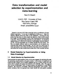
obtaining a boolean stream P , called the paper folding stream, in which top folds and valley folds are represented by 0 and 1, respectively. Imagine what happens if we do an extra fold. Then all existing folds remain, but between every two consecutive folds a new fold is created. These new folds are alternately top folds and valley folds. So the effect of folding once more is that the new sequence is the zip of 010101 · · · and the old sequence. Taking the limit we obtain P = zip(alt, P ), where for zip and alt we have the equations zip(x : σ, τ ) = x : zip(τ, σ), alt = 0 : 1 : alt. One may wonder whether P is already fully defined by these three equations for P , zip and alt. It is, by Theorem 5.1, since the equations form a proper stream specification Rs for which termination of Obs(Rs ) is easily proved by TTT2 or AProVE. Paper folding and many of its properties is folklore; we found this characterization of P independently. Turtle visualization of P is of particular interest, since the result is not just a visualization, but also the shape obtained if the ribbon is not fully unfolded, but only unfolded until the angles given as parameter of the turtle visualization. We only consider the case where the angles for 0 (top fold) and 1 (valley fold) are equal. In case this angle is 90 degrees, then the result is called the dragon curve; this curve touches itself, but does not intersect itself. Pictures are easily found on the Internet. When choosing turtle angles of less than 90 degrees, that is, the remaining paper fold is greater than 90 degrees, then the curve neither touches nor intersects itself. Doing this for 87 degrees and doing 15 folds, this yields the following turtle visualization of the first 215 − 1 = 32767 elements of the stream P:

18

HANS ZANTEMA

7. Data Independent Stream Functions The reason that in Theorem 5.1 we have to restrict to models satisfying S = {[t] | t ∈ Ts }, as we saw in Example 3, is in the fact that computations may be guarded by data elements in left-hand sides of equations. Next we show that we also get well-definedness for stream functions defined on all streams in case the left-hand sides of the equations do not contain data elements. Theorem 7.1. Let (Σd , Σs , Rd , Rs ) be a proper stream specification for which the TRS Obs(Rs ) ∪ Rd is terminating and the only subterms of left-hand sides of Rs of sort d are variables. Then the stream specification admits a unique model (S, ([f ])f ∈Σs ) satisfying S = Dω . Proof. (sketch) We have to prove that for any f ∈ Σs of type dn × sm → s the function [f ] : Dn × (Dω )m → Dω is uniquely defined. For doing so we introduce m fresh constants c1 , . . . , cm of sort s. Let k ∈ N and u1 , . . . , un ∈ D. Due to termination and orthogonality of Obs(Rs ) ∪ Rd , the term head(tailk (f (u1 , . . . , un , c1 , . . . , cm ))) has a unique normal form with respect to Obs(Rs ) ∪ Rd . Since it is of sort d, due to the shape of the rules it is a ground term of sort d over Σd ∪ {head, tail, c1 , . . . , cm }, that is, a ground term T composed from Σd and terms of the shape head(taili (cj )) for i ∈ N and j ∈ {1, . . . , m}. For this observation it is essential that left-hand sides do not contain non-variable terms of sort d: terms of the shape f (head(· · · ), · · · ) should be rewritten. Let N be the greatest number i for which T has a subterm of the shape head(taili (cj )). Let s1 , . . . , sm ∈ Dω . Define tj = sj (0) : sj (1) : · · · : sj (N ) : σ. Since the term head(tailk (f (u1 , . . . , un , c1 , . . . , cm ))) rewrites to T , head(tailk (f (u1 , . . . , un , t1 , . . . , tm ))) rewrites to T 0 obtained from T by replacing every subterm of the shape head(taili (cj )) by head(taili (tj )). Observe that head(taili (tj )) rewrites to sj (i) ∈ D. So ([f ](u1 , . . . , un , s1 , . . . , sm ))(k) has to be the Rd -normal form of the ground term over Σd obtained from T by replacing every subterm of the shape head(taili (cj )) by sj (i) ∈ D. Since this fixes ([f ](u1 , . . . , un , s1 , . . . , sm ))(k) for every k, this uniquely defines [f ]. Example 6. It is easy to see that for the standard stream functions zip, even and odd defined by even(x : σ) = x : odd(σ), odd(x : σ) = even(σ), zip(x : σ, τ ) = x : zip(τ, σ), there exists f : Dω → Dω for every data set D satisfying f (x : σ) = x : zip(f (even(σ)), f (odd(σ))), namely the identity. By Theorem 7.1 we can conclude it is the only one, since for Rd = ∅ and Rs consisting of the above four equations, the resulting TRS Obs(Rs ) consisting of the rules head(even(σ)) → head(σ) head(odd(σ)) → head(even(tail(σ))) tail(even(σ)) → odd(tail(σ)) tail(odd(σ)) → tail(even(tail(σ))) head(f (σ)) → head(σ) tail(f (σ)) → zip(f (even(tail(σ))), f (odd(tail(σ)))) and the rules for ’:’ and zip as in Example 2, is terminating as can be proved by AProVE [6] or TTT2 [10]. Other approaches seem to fail: the technique from [16] fails to prove that the identity is the only stream function satisfying the equation for f , while productivity of


19

stream specifications containing the rule for f cannot be proved to be productive by the technique from [4]. By essentially choosing Obs(Rs ) as the input and adding information about special contexts, the tool Circ [11] is able to prove that f is the identity.

8. More Transformations Preserving Semantics Unfolding the Fibonacci stream specification as given in the introduction yields the proper stream specification Rs consisting of the equations Fib = f (Fib) f (x : σ) = g(x, σ)

g(0, σ) = 0 : 1 : f (σ) g(1, σ) = 0 : f (σ).

However, the TRS Obs(Rs ) is not terminating since it allows the infinite reduction tail(Fib) → tail(f (Fib)) → tail(g(head(Fib), tail(Fib))) → · · · , | {z } so our method fails to prove well-definedness of Fib in a direct way. In Lemma 3.2 and Lemma 3.3 we already saw two ways to modify stream specifications while preserving their semantics. In this section we will extend these lemmas to more general semantics preserving transformations, in particular by making use of the equations E from the proof of Lemma 5.5 that hold in every model. As an example, we will apply such transformations to our original Fib specification. The observational variant of the resulting stream specification will be terminating, so proving well-definedness of the transformed Fib specification. But since the transformations are semantics preserving, this also proves well-definedness of the original Fib specification. In general we propose the following approach: in case for a stream specification the termination tools fail to prove termination of the observational variant, then try to apply semantics preserving transformations as discussed in Section 3 and this section until a transformed system has been found for which termination of the observational variant can be proved. If this succeeds, this not only proves well-definedness of the transformed specification, but also of the original one. In this approach we have a symbol tail in several variants of the specification, while in the construction of observational variant a fresh symbol tail is required. So in the observational variant two versions of tail occur: the original symbol tail and the symbol tail created by Obs. However, if the observational variant happens to be terminating after identifying these two versions of tail, then it is also terminating if they are distinguished, so identifying them will not yield wrong results. But it may happen that termination holds if the two versions of tail are distinguished, and does not hold if they are identified. This is the case for Example 2. Recall that mapping a stream specification (Σd , Σs , Rd , Rs ) to (Σd , Σ0s , Rd , Rs0 ) with Σs ⊆ Σ0s is said to preserve semantics if • (Σd , Σs , Rd , Rs ) is well-defined if and only if (Σd , Σ0s , Rd , Rs0 ) is well-defined, and • If (Σd , Σs , Rd , Rs ) is well-defined with corresponding model (S, [·]), and (S 0 , [·]0 ) is the model corresponding to (Σd , Σ0s , Rd , Rs0 ), then [t] = [t]0 for all ground terms of sort s over Σd ∪ Σs . For well-definedness we required the model to satisfy S = {[t] | t ∈ Ts }. For this section we need one more technical requirement: S should be closed under tail. In order not to

20

HANS ZANTEMA

change our definitions, throughout this section we assume the following extra assumptions to achieve this requirement: • the symbol tail is in Σs , and • the corresponding equation tail(x : σ) = σ is in Rs . Lemma 3.3 states that in keeping the same signature Σs , replacing Rs by Rs0 preserves semantics as long as convertibility with respect to Rs coincides with convertibility with respect to Rs0 . But as we are interested in preservation of semantics, this syntactical convertibility requirement may be weakened to a more semantic version: if Rs and Rs0 do not have the same convertibility relation, but allow the same models, the same can be concluded. So now for a set Rs of equations we will introduce a congruence ∼Rs being weaker than =Rs , but still preserving semantics. Recall the set E of equations   head(x : σ) = x tail(x : σ) = σ E=  σ = head(σ) : tail(σ) For a set Rs of equations of sort s we define the relation ∼Rs on terms over Σs ∪Σd ∪{head} inductively by • if ` = r is in Rs then ` ∼Rs r, • ∼Rs is reflexive, symmetric and transitive, • if C is a context and ρ is a substitution and t ∼Rs t0 , then C[tρ] ∼Rs C[t0 ρ], • if ` = r is in E then ` ∼Rs r, • if t, t0 are terms that may contain a fresh variable x of type d, and t[x := u] ∼Rs t0 [x := u] for every u ∈ D, then t ∼Rs t0 . Note that =Rs is defined by the first three items, so ∼Rs generalizes =Rs by the additional last two items. Lemma 8.1. Let (Σd , Σs , Rd , Rs ) and (Σd , Σs , Rd , Rs0 ) be stream specifications satisfying ` ∼Rs0 r for all ` = r in Rs , and ` ∼Rs r for all ` = r in Rs0 . Then transforming (Σd , Σs , Rd , Rs ) to (Σd , Σs , Rd , Rs0 ) preserves semantics. Proof. In an arbitrary model (S, [·]) for a stream specification we define [head](s) = s(0) for s ∈ S ⊆ Dω . By assuming the equation tail(x : σ) = σ we conclude ([tail](s))(i) = s(i + 1) for i ≥ 0. Combined with the definition of [:] we conclude that E holds in every model. In case an equation t[x := u] = t0 [x := u] holds in a model for every u ∈ D, then by definition the equation t = t0 holds in the model, too. Combining these observations we conclude by induction on the structure of ∼Rs that if a model satisfies Rs , and t ∼Rs t0 , then the model satisfies the equation t = t0 too. Applying this both for ∼Rs and ∼Rs0 , and using the conditions of the lemma we conclude that a model satisfies (Σd , Σs , Rd , Rs ) if and only if it satisfies (Σd , Σs , Rd , Rs0 ). From this the lemma follows. Example 7. Our Fib specification completed by the tail equation reads f (0 : σ) = 0 : 1 : f (σ) f (1 : σ) = 0 : f (σ)

Fib = f (Fib) tail(x : σ) = σ.


21

By Theorem 3.4 we know that unfolding this to f (x : σ) = g(x, σ) g(0, σ) = 0 : 1 : f (σ) g(1, σ) = 0 : f (σ)

Fib = f (Fib), tail(x : σ) = σ

preserves semantics. Moreover, by Lemma 3.2 we may add a constant c to the signature and add the equation c = tail(Fib), still preserving semantics. Let Rs consist of these equations, and let Rs0 consist of f (x : σ) = g(x, σ) g(0, σ) = 0 : 1 : f (σ) g(1, σ) = 0 : f (σ)

Fib = 0 : c c = 1 : f (c) tail(x : σ) = σ.

Now we will check the conditions of Lemma 8.1. For proving that ` ∼Rs0 r for all ` = r in Rs we only need to consider the equations c = tail(Fib) and Fib = f (Fib). We obtain c =Rs0 tail(0 : c) =Rs0 tail(Fib) and Fib =Rs0 0 : c =Rs0 0 : 1 : f (c) =Rs0 g(0, c) =Rs0 f (0 : c) =Rs0 f (Fib). For proving ` ∼Rs r for all ` = r in Rs0 we only need to consider the equations Fib = 0 : c and c = 1 : f (c). For this we need the congruence ∼Rs rather than =Rs . First observe head(g(0, σ)) ∼Rs head(0 : 1 : f (σ)) ∼Rs 0, and head(g(1, σ)) ∼Rs head(0 : f (σ)) ∼Rs 0, so by the last item of the definition of ∼Rs we obtain head(g(x, σ)) ∼Rs 0. Using this we get Fib ∼Rs head(Fib) : tail(Fib) ∼Rs head(Fib) : c ∼Rs head(f (Fib)) : c ∼Rs head(f (head(Fib) : tail(Fib))) : c ∼Rs head(g(head(Fib), tail(Fib))) : c ∼Rs 0 : c. Using Fib ∼Rs 0 : c, for the remaining equation we have c ∼Rs ∼Rs ∼Rs ∼Rs ∼Rs ∼Rs

tail(Fib) tail(f (Fib)) tail(f (0 : c)) tail(g(0, c)) tail(0 : 1 : f (c)) 1 : f (c).

So the requirements of Lemma 8.1 are fulfilled and we conclude that transforming Rs to Rs0 preserves semantics. By tools like AProVE or TTT2 one proves that Obs(Rs0 ) is terminating, so by Theorem 5.1 Rs0 is well-defined. Due to preservation of semantics the same holds for Rs , and for the original Fib specification.

22

HANS ZANTEMA

As a consequence, we can conclude incompleteness of Theorem 5.1: the stream specification Rs is well-defined but Obs(Rs ) is not terminating, due to the infinite reduction of Obs(Rs ) we saw before. The argument for the Fib example can be given in a more sloppy way as was done in [19] as follows. Identify ground terms with their interpretations in a model. The result of g always starts by 0, so we can write Fib = f (Fib) = g(· · · ) = 0 : c for some stream c. Using this equality Fib = 0 : c we obtain 0 : c = Fib = f (Fib) = f (0 : c) = 0 : 1 : f (c), so c = 1 : f (c). So any model for the original specification also satisfies Rs0 which is obtained by replacing the equation Fib = f (Fib) by the two equations Fib = 0 : c and c = 1 : f (c). As Rs0 satisfies our format and Obs(Rs0 ) is terminating we conclude well-definedness of Fib. For justifying the steps f (Fib) = g(· · · ) = 0 : c in this argument we need the last two items of the definition of ∼Rs : • for the step f (Fib) = g(· · · ) we need E to rewrite Fib to a term with ”:” on top, and • for the step g(· · · ) = 0 : c we need the case analysis on the data element in ”· · · ” as expressed by the last item in the definition of ∼Rs , exactly as we did in our detailed proof. Note that the sloppy argument only shows that the new equations in Rs0 are implied by original equations, and not the other way around. The following example shows that it is essential also to prove the other direction. Example 8. Consider the proper stream specification Rs consisting of f (x : σ, y : τ ) g(0, 0) g(0, 1) g(1, x)

= = = =

g(x, y) ones zeros zeros

zeros ones c tail(x : σ)

= = = =

0 : zeros 1 : ones f (c, c) σ

If [c] starts with 0, then [f (c, c)] = [g(0, 0)] = [ones] starts with 1, and if [c] starts with 1, then [f (c, c)] = [g(1, 1)] = [zeros] starts with 0, so Rs does not admit a model and is not well-defined. However, the proper stream specification Rs0 obtained from Rs by replacing c = f (c, c) by c = f (f (c, c), c) is well-defined, while this new equation satisfies c =Rs f (f (c, c), c). Well-definedness of Rs0 can be proved by proving termination of Obs(Rs00 ), where Rs00 is obtained from Rs0 by replacing the equation for c by c = zeros. The transformation from Rs0 to Rs00 satisfies the requirements of Lemma 8.1; for checking this one shows that f (f (0 : σ, 0 : σ), 0 : σ) ∼Rs0 f (g(0, 0), 0 : σ) ∼Rs0 f (1 : ones, 0 : σ) ∼Rs0 g(1, 0) ∼Rs0 zeros and f (f (1 : σ, 1 : σ), 1 : σ) ∼Rs0 f (g(1, 1), 1 : σ) ∼Rs0 f (0 : zeros, 1 : σ) ∼Rs0 g(0, 1) ∼Rs0 zeros by which from the last item of the definition of ∼Rs0 one concludes f (f (x : σ, x : σ), x : σ) ∼Rs0 zeros, hence c ∼Rs0 f (f (c, c), c) ∼Rs0 f (f (head(c) : tail(c), head(c) : tail(c)), head(c) : tail(c)) ∼Rs0 zeros.


23

Next we show how we can use the combination of Lemmas 3.2 and 8.1 and Theorem 5.1 to prove that the following stream specification admits exactly two models (S, [·]) with S = {[t] | t ∈ Ts }: f (0 : σ) = 0 : 1 : f (σ) f (1 : σ) = 1 : 0 : f (σ)

m = f (m) tail(x : σ) = σ.

Assume we have a model (S, [·]) of this specification. Then either [m](0) = 0 or [m](0) = 1. In the former case the equation m = 0 : tail(m) holds, in the latter case the equation m = 1 : tail(m) holds. First assume we are in the former case. Then we may add the equation m = 0 : tail(m). For this extended system we will prove well-definedness. Note that the specification is not orthogonal, but for applying Lemmas 3.2 and 8.1 and Theorem 3.4 this is not required. After applying Lemma 3.2 and Theorem 3.4 we arrive at the (non-proper) specification Rs consisting of f (x : σ) = g(x, σ) g(0, σ) = 0 : 1 : f (σ) g(1, σ) = 1 : 0 : f (σ)

m m c tail(x : σ)

= = = =

f (m) 0 : tail(m) tail(m) σ.

Now we transform this to the proper specification Rs0 consisting of f (x : σ) = g(x, σ) g(0, σ) = 0 : 1 : f (σ) g(1, σ) = 1 : 0 : f (σ)

m = 0:c c = 1 : f (c) tail(x : σ) = σ.

One easily checks that ` =Rs0 r for all equations ` = r in Rs and conversely, so by Lemma 8.1 (or even Lemma 3.3) one concludes that this transformation is semantics preserving. Since Obs(Rs0 ) is easily checked to be terminating, this shows that adding m = 0 : tail(m) to the original specification yields exactly one model with S = {[t] | t ∈ Ts }. By symmetry the same holds for the other case, where the equation m = 1 : tail(m) is added. Without a proof we mention that the two solutions for m are exactly the Thue-Morse stream morse from Example 1 and its inverse. We conclude this section by an elaboration of the Kolakoski stream. Example 9. The Kolakoski stream Kol is the unique fix point of g defined by g(0 : σ) g(1 : σ) f (0 : σ) f (1 : σ)

= = = =

1 : 1 : f (σ) 1 : f (σ) 0 : 0 : g(σ) 0 : g(σ).

So both for f and g its result on a stream is defined as follows. If a 1 is read, then a single symbol is produced, and if a 0 read, then two copies of a symbol are produced. This producing is done in such a way that the produced elements are alternately 0’s and 1’s, for f starting with 0 and for g starting with 1. Due to this procedure in some presentations instead of 0 the number 2 is written. Of course we have to prove that g has a unique fix point Kol. Similar to what we saw for Fib, the fix point equation Kol = g(Kol) causes non-termination in the observational variant so we cannot apply our approach directly. In order to prove well-definedness, we follow the same lines as we did for Fib, with the difference that now we do not start by unfolding, but postpone unfolding to the end. Start by the four equations for f and g, and the equations Kol = g(Kol) and tail(x : σ) = σ. According to Lemma 3.2 addition of

24

HANS ZANTEMA

the equation K = tail(tail(Kol)) is semantics preserving. So let Rs consist of all of these equations for f, g, Kol, tail, K. We will transform this to Rs0 consisting of the equations for f, g, tail, and the two equations Kol = 1 : 0 : K, K = 0 : g(K). Applying unfolding (Theorem 3.4) to Rs0 yields a proper stream specification for which TTT2 and AProVE succeed in proving termination of the observational variant, so by Lemma 8.1 it remains to show that ` ∼Rs0 r for all ` = r in Rs , and ` ∼Rs r for all ` = r in Rs0 . For doing so, first we show that head(g(0 : σ)) ∼Rs 1 and head(g(1 : σ)) ∼Rs 1, so head(g(x : σ)) ∼Rs 1, and hence head(g(σ)) ∼Rs head(g(head(σ) : tail(σ))) ∼Rs 1. Similarly we obtain head(f (σ)) ∼Rs 0. Using this we derive Kol ∼Rs head(Kol) : tail(Kol) ∼Rs head(g(Kol)) : tail(Kol) ∼Rs 1 : tail(Kol), and head(tail(Kol)) ∼Rs head(tail(g(Kol))) ∼Rs head(tail(g(1 : tail(Kol)))) ∼Rs head(tail(1 : f (tail(Kol)))) ∼Rs head(f (tail(Kol))) ∼Rs 0 from which Kol ∼Rs 1 : 0 : K follows. Moreover, we obtain K ∼Rs ∼Rs ∼Rs ∼Rs ∼Rs ∼Rs ∼Rs

tail(tail(Kol)) tail(tail(g(Kol))) tail(tail(g(1 : 0 : K))) tail(tail(1 : f (0 : K))) tail(f (0 : K)) tail(0 : 0 : g(K)) 0 : g(K).

For the other direction we have g(Kol) ∼Rs0 g(1 : 0 : K) ∼Rs0 1 : f (0 : K) ∼Rs0 1 : 0 : 0 : g(K) ∼Rs0 1 : 0 : K ∼Rs0 Kol and K ∼Rs0 tail(tail(1 : 0 : K)) ∼Rs0 tail(tail(Kol)), concluding the proof. Although this stream Kol has a very simple and regular definition, the stream seems to behave remarkably irregular. In contrast to earlier streams we saw, turtle visualizations of Kol show up hardly any regular pattern: they seem to behave just like randomly generated boolean streams. For instance, by choosing the angle to be 90 degrees both for 0 and 1, taking the first 50000 elements of Kol yields the following turtle visualization:


25

9. Conclusions and Further Research We presented a technique by which well-definedness of stream specifications like Example 3 can be proved fully automatically, where a tool like Circ [12, 11] fails, and the productivity tool [4] fails to prove productivity. The main idea is to prove well-definedness by proving termination of a transformed system Obs(Rs ), in this way exploiting the power of present termination provers. We observed that productivity of the stream specification cannot be concluded from termination of Obs(Rs ). Intuitively, productivity is closely related to termination; we leave as a challenge to further relate termination with productivity of stream specifications. A first step in this direction was made in [21]. There it was proved that productivity of a stream specification is equivalent to balanced outermost termination of the specification extended by an extra rule x : σ → overflow. Here an infinite reduction is called balanced outermost if only outermost redexes are reduced, and in the choice of them some fairness condition holds. As there are powerful techniques to prove outermost termination automatically [5], this can be used to prove productivity fully automatically. Unfortunately, as soon as binary operations like zip come in, typically the notions outermost termination and balanced outermost termination do not coincide: for many productive stream specifications the extension by the overflow rule is not outermost terminating, by which this approach fails. Instead in [20] some basic criteria for productivity have been investigated together with relationship with context-sensitive termination. Combined with a number of transformations and corresponding heuristics, this yields a powerful technique for proving productivity automatically, supported by an implementation. This approach exploits the power of present termination provers for proving productivity, just like we do in this paper for proving well-definedness. We offer an implementation for computing Obs(Rs ) automatically, by which proving well-definedness can be done fully automatically in case the approach applies directly. For cases for which the approach does not apply directly, in Section 3 and Section 8 we developed techniques to transform stream specifications in such a way that semantics and welldefinedness is preserved, and often our approach applies to the transformed specifications. Among these techniques only unfolding (Theorem 3.4) is supported by our implementation. For the other techniques some heuristics will be required. For the Fibonacci stream (Example 7) and the Kolakoski stream (Example 9) the following heuristics turned out to be successful: • Identify a non-productive constant c. In both mentioned examples this is the stream to be defined, for which the equation is of the shape c = f (c). • Determine the first element d of the stream represented by c. • Introduce a fresh constant c0 , and introduce the equation c = d : c0 . • Using both the original equations and this new equation c = d : c0 try to find a sound equation c0 = t in which t is a term containing c0 , but not c. • Replace the original equation c = · · · by the two new equations c = d : c0 and c0 = t, and check whether this transformation is semantics preserving. • In case this approach fails, try the generalization in which the first n elements d1 , . . . , dn of the stream represented by c are determined for some small value n, and the equation c = d1 : d2 : · · · : dn : c0 is introduced for a fresh constant c0 . Another approach of using the techniques of Section 3 and Section 8 is proving welldefinedness of a stream specification by proving productivity of all ground terms in a

26

HANS ZANTEMA

transformed specification, e.g., by the approach of [20]. Since productivity implies welldefinedness and the transformation preserves semantics, this implies well-definedness of the original specification. In Section 8 we used the technical assumption that the model is closed under tail. This was forced by assuming the equation tail(x : σ) = σ. We conjecture that for the validity of the approach this is not essential. More precisely, we conjecture that a stream specification (Σd , Σs , Rd , Rs ) with tail 6∈ Σs is well-defined if and only if the extended specification (Σd , Σs ∪ {tail}, Rd , Rs ∪ {tail(x : σ) = σ}) is well-defined. This looks trivial as tail does not occur in the original specification, so is not expected to influence anything. However, giving a formal proof causes problems. The reason is that the model for (Σd , Σs , Rd , Rs ) may not be closed under [tail]. In fact we can even prove that in the model (S, [·]) for the Fib example satisfying S = {[t] | t ∈ Ts }, the tail of Fib is not contained in S. A problem is how to lift [f ] defined on S to the larger model that is closed under tail. For the particular Fib example a solution can be given, but for the general setting we failed. This paper purely focuses on streams over a fixed data set D; in all examples even D consists of the booleans. It is expected that the approach can be generalized to other infinite data types like infinite binary trees. A suitable format for this more general kind of infinite data structures has been given in [20]. In such a setting destructors can be defined as inverses of the constructors, just like in this paper we introduced (head, tail) as the inverse of ’:’. Similar to what we did in this paper for streams, in this more general setting a specification consisting of equations on terms over constructors and user defined symbols will be transformed to an observational variant, being a rewrite system over destructors and the user defined symbols. Just like we did in this paper for the special case of streams, this rewrite system serves for observing data. It is orthogonal by construction, and welldefinedness can be concluded from termination. Although the agenda for this approach for other infinite data structures is similar to what we did in this paper, this has not been elaborated in detail. References [1] J.-P. Allouche and J. Shallit. Automatic Sequences: Theory, Applications, Generalizations. Cambridge University Press, 2003. [2] T. Arts and J. Giesl. Termination of term rewriting using dependency pairs. Theoretical Computer Science, 236:133–178, 2000. [3] F. Baader and T. Nipkow. Term Rewriting and All That. Cambridge University Press, 1998. [4] J. Endrullis, C. Grabmayer, and D. Hendriks. Data-oblivious stream productivity. In Proceedings of the 11th International Conference on Logic for Programming, Artificial Intelligence, and Reasoning (LPAR’08), volume 5330 of Lecture Notes in Computer Science, pages 79–96. Springer, 2008. webinterface tool: http://fspc282.few.vu.nl/productivity/. [5] J. Endrullis and D. Hendriks. From outermost to context-sensitive rewriting. In R. Treinen, editor, Proceedings of the 20th Conference on Rewriting Techniques and Applications (RTA), volume 5595 of Lecture Notes in Computer Science, pages 305–319. Springer, 2009. [6] J. Giesl, P. Schneider-Kamp, and R. Thiemann. AProVE 1.2: Automatic termination proofs in the dependency pair framework. In Proceedings of the 3rd International Joint Conference on Automated Reasoning (IJCAR ’06), volume 4130 of Lecture Notes in Computer Science, pages 281–286. Springer, 2006. Tool available at http://aprove.informatik.rwth-aachen.de/. [7] J. Giesl, R. Thiemann, and P. Schneider-Kamp. The dependency pair framework: Combining techniques for automated termination proofs. In Franz Baader and Andrei Voronkov, editors, Proceedings


[8]

[9]

[10]

[11]

[12] [13]

[14]

[15] [16] [17]

[18]

[19]

[20]

[21]

27

of the 11th International Conference on Logic for Programming, Artificial Intelligence, and Reasoning (LPAR’04), volume 3452 of Lecture Notes in Artificial Intelligence, pages 301–331, Montevideo, Uruguay, 2005. Springer. J. Goguen, K. Lin, and G. Rosu. Circular coinductive rewriting. In Proceedings, 15th International Conference on Automated Software Engineering (ASE’00). Institute of Electrical and Electronics Engineers Computer Society, 2000. Grenoble, France, 11-15 September 2000, webinterface tool CIRC: http://fsl.cs.uiuc.edu/index.php/Special:CircOnline. R. Hinze. Functional pearl: streams and unique fixed points. In J. Hook and P. Thiemann, editors, Proceeding of the 13th ACM SIGPLAN international conference on Functional programming, ICFP 2008, pages 189–200. ACM, 2008. M. Korp, C. Sternagel, H. Zankl, and A. Middeldorp. Tyrolean termination tool 2. In R. Treinen, editor, Proceedings of the 20th Conference on Rewriting Techniques and Applications (RTA), Lecture Notes in Computer Science. Springer, 2009. Tool available at http://colo6-c703.uibk.ac.at/ttt2/. D. Lucanu, E.-I. Goriac, G. Caltais, and G. Rosu. CIRC: A behavioral verification tool based on circular coinduction. In Proceedings of the 3rd Conference on Algebra and Coalgebra in Computer Science (CALCO’09), volume 5728 of Lecture Notes in Computer Science, pages 433–442. Springer, 2009. D. Lucanu and G. Rosu. CIRC: A circular coinductive prover. In CALCO’07, volume 4624 of Lecture Notes in Computer Science, pages 372 – 378, 2007. D. Lucanu and G. Rosu. Circular coinduction: A proof theoretical foundation. In Proceedings of the 3rd Conference on Algebra and Coalgebra in Computer Science (CALCO’09), volume 5728 of Lecture Notes in Computer Science, pages 127–144. Springer, 2009. C. Marche and H. Zantema. The termination competition. In F. Baader, editor, Proceedings of the 18th Conference on Rewriting Techniques and Applications (RTA), volume 4533 of Lecture Notes in Computer Science, pages 303–313. Springer, 2007. G. Ro¸su. Equality of streams is a Π02 -complete problem. In Proceedings of the 11th ACM SIGPLAN International Conference on Functional Programming (ICFP’06). ACM, 2006. J.J.M.M. Rutten. A coinductive calculus of streams. Mathematical Structures in Computer Science, 15:93–147, 2005. J. G. Simonsen. The Π02 -completeness of most of the properties of rewriting systems you care about (and productivity). In R. Treinen, editor, Proceedings of the 20th Conference on Rewriting Techniques and Applications (RTA), Lecture Notes in Computer Science. Springer, 2009. H. Zantema. A tool proving well-definedness of streams using termination tools. In Proceedings of the 3rd Conference on Algebra and Coalgebra in Computer Science (CALCO’09), volume 5728 of Lecture Notes in Computer Science, pages 449–456. Springer, 2009. H. Zantema. Well-definedness of streams by termination. In R. Treinen, editor, Proceedings of the 20th Conference on Rewriting Techniques and Applications (RTA), volume 5595 of Lecture Notes in Computer Science, pages 164–178. Springer, 2009. H. Zantema and M. Raffelsieper. Proving productivity in infinite data structures. In C. Lynch, editor, Proceedings of the 21st Conference on Rewriting Techniques and Applications (RTA), Leibniz International Proceedings in Informatics. Schloss Dagstuhl Publishing, 2010. H. Zantema and M. Raffelsieper. Stream productivity by outermost termination. In Proceedings of the 9th International Workshop in Reduction Strategies in Rewriting and Programming (WRS 09), volume 15 of Electronic Proceedings in Theoretical Computer Science, 2010.

This work is licensed under the Creative Commons Attribution-NoDerivs License. To view a copy of this license, visit http://creativecommons.org/licenses/by-nd/2.0/ or send a letter to Creative Commons, 171 Second St, Suite 300, San Francisco, CA 94105, USA, or Eisenacher Strasse 2, 10777 Berlin, Germany