and multivariate analysis, degrees of freedom are a function of sample size, number ... or a parameter are called the degrees of freedom {dfi. (HyperStat Online, n.d.). For example,a ..... sciences (2nd ed.), Belmont ... com/computer/sas/df.hnnl.
RESEARCH NOTE
What Are Degrees of Freedom? Shanta Pandey and Charlotte Lyn Bright
A
S we were teaching a multivariate statistics course for doctoral students, one of the students in the class asked,"What are degrees of freedom? I know it is not good to lose degrees of freedom, but what are they?" Other students in the class waited for a clear-cut response. As we tried to give a textbook answer, we were not satisfied and we did not get the sense that our students understood. We looked through our statistics books to determine whether we could find a more clear way to explain this term to social work students.The wide variety of language used to define degrees ojfrecdom is enough to confuse any social worker! Definitions range from the broad, "Degrees of freedom are the number of values in a distribution that are free to vary for any particular statistic" (Healey, 1990, p. 214), to the technical; Statisticians start with the number of terms in the sum [of squares], then subtract the number of mean values that were calculated along the way. The result is called the degrees of freedom, for reasons that reside, believe it or not. in the theory of thermodynamics. (Norman & Streiiier, 2003, p. 43) Authors who have tried to be more specific have defined degrees of freedom in relation to sample size (Trochim,2005;Weinbach & Grinne]],2004), cell size (Salkind, 2004), the mmiber of relationships in the data (Walker, 1940),and the difference in dimensionahties of the parameter spaces (Good, 1973).The most common definition includes the number or pieces of information that are free to vary (Healey, 1990; Jaccard & Becker, 1990; Pagano, 2004; Warner, 2008; Wonnacott & Wonnacott, 1990). These specifications do not seem to augment students' understanding of this term. Hence, degrees of freedom are conceptually difficult but are important to report to understand statistical analysis. For example, without degrees of freedom, we are unable to calculate or to understand any
CCCCode: 107O-S3O9/O8 (3.00 O2008 National Association of Sotial Workers
underlying population variability. Also, in a bivariate and multivariate analysis, degrees of freedom are a function of sample size, number of variables, and number of parameters to be estimated; therefore, degrees of freedom are also associated with statistical power. This research note is intended to comprehensively define degrees of freedom, to explain how they are calculated, and to give examples of the different types of degrees of freedom in some commonly used analyses. DEGREES OF FREEDOM DEFINED
In any statistical analysis the goal is to understand how the variables (or parameters to be estimated) and observations are linked. Hence, degrees of freedom are a function of both sample size (N) (Trochim, 2005) and the number of independent variables (k) in one's model (Toothaker & Miller, 1996; Walker, 1940; Yu, 1997).The degrees of fi^edom are equal to the number of independent observations {N),or the number of subjects in the data, minus the number of parameters (k) estimated (Toothaker & Miller, 1996; Walker, 1940). A parameter (for example, slope) to be estimated is related to the value of an independent variable and included in a statistical equation (an additional parameter is estimated for an intercept iu a general linear model). A researcher may estimate parameters using different amounts or pieces of information,and the number of independent pieces of information he or she uses to estimate a statistic or a parameter are called the degrees of freedom {dfi (HyperStat Online, n.d.). For example,a researcher records income of N number of individuals from a community. Here he or she has Nindependent pieces of information (that is, N points of incomes) and one variable called income (t); in subsequent analysis of this data set, degrees of freedom are asociated with both Nand k. For instance, if this researcher wants to calculate sample variance to understand the extent to which incomes vary in this community, the degrees of freedom equal N - fc.The relationship between sample size and degrees of freedom is
119
positive; as sample size increases so do the degrees of freedom. On the other hand, the relationship between the degrees of freedom and number of parameters to be estimated is negative. In other words, the degrees of freedom decrease as the number of parameters to be estimated increases. That is why some statisticians define degrees of freedom as the number of independent values that are left after the researcher has applied all the restrictions (Rosenthal, 2001; Runyon & Haber, 1991); therefore, degrees of freedom vary from one statistical test to another (Salkind, 2004). For the purpose of clarification, let us look at some examples. A Single Observation with One Parameter to Be Estimated If a researcher has measured income (k = 1) for one observation {N = 1) from a community, the mean sample income is the same as the value of this observation. With this value, tbe researcher has some idea ot the mean income of this community but does not know anything about the population spread or variability (Wonnacott & Wonnacott, 1990). Also, the researcher has only one independent observation (income) with a parameter that he or she needs to estimate. The degrees of freedom here are equal to N - fc.Thus, there is no degree of freedom in this example (1 - 1 = 0). In other words, the data point has no freedom to vary, and the analysis is limited to the presentation of the value of this data point (Wonnacott & Wonnacott, 1990; Yu, 1997). For us to understand data variability, N must be larger than 1. Multiple Observations (N) with One Parameter to Be Estimated Suppose there are N observations for income. To examine the variability in income, we need to estimate only one parameter (that is, sample variance) for income (k), leaving the degrees of freedom of N — k. Because we know that we have only one parameter to estimate, we may say that we have a total of N — 1 degrees of freedom. Therefore, all univariate sample characteristics that are computed with the sum of squares including the standard deviation and variance have N— 1 degrees of freedom (Warner, 2008). Degrees of freedom vary from one statistical test to another as we move from univariate to bivariate and mtiltivariate statistical analysis, depending on the nature of restrictions applied even when
120
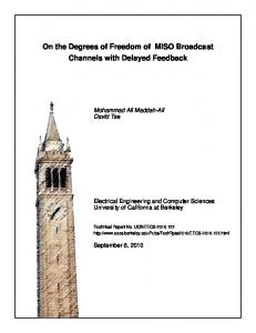
sample size remains unchanged. In the examples that follow, we explain how degrees of freedom are calculated in some of the commonly used bivariate and muJtivariate analyses. 1Wo Samples with One Parameter (or t Test) Suppose that the researcher has two samples, men and women, or n, + n^ observations. Here, one can use an independent samples t test to analyze whether the mean incomes of these two groups are different. In the comparison of income variability between these two independent means (or k number of means), the researcher will have n^ + n.,-2 degrees of freedom. The total degrees of freedom are the sum of the number of cases in group 1 and group 2 minus the number of groups. As a case in point, see the SAS and SPSS outputs of a t test comparing the literacy rate (LITERACY, dependent variable) of poor and rich countries (GNPSPLIT, independent variable) in Table l.AU in all, SAS output has four different values of degrees offreedom(two of which are also given by SPSS).We review each of them in the following paragraphs. The first value for degrees of freedom under t tests is 100 (reported by both SAS and SPSS).The two groups of countries (rich and poor) are assumed to have equal variances in their literacy rate, the dependent variable. This first value of degrees of freedom is calculated as M^ + n^-2 (the sum of the sample size of each group compared in the f test minus the number of groups being compared), that is.64 + 3 8 - 2 = 100. For the test of equality of variance, both SAS and SPSS use the F test. SAS uses two different values of degrees of freedom and reports folded F statistics. The numerator degrees of freedom are calculated as n — 1, that is 64 — 1 = 63. The denominator degrees of freedom are calculated as n^ - 1 or 38 - 1 = 37.These degrees of freedom are used in testing the assumption that the variances in the two groups (rich and poor countries, in our example) are not significantly different.These two values are included in the calculations computed within the statistical program and are reported on SAS output as shown in Table 1. SPSS, however, computes Levene's weighted F statistic (seeTable 1) and uses k-\ and N - kdegrees offreedom,where k stands for the number of groups being compared and N stands for the total number of observations in the sample; therefore, the degrees of freedom associated with the Levene's F statistic
Social Work Research VOLUME J I , NUMBER Z
JUNE ZOO8
GNPSPLiT 0 (poor) 1 [rich)
46.563 88.974
00 00
>^
lA
^3
I 13
1a LITERACY
LITERACY Equal variances assumed Equal variances not assumed
LITERACT
14,266
T
o
o tt; Q IT
1 u 'O c
UJ
rj
1
.3
-TJ (N rS oS
cv r^ fS -«•
Q
00
p
S
Q
C-
lA
I. 2 Q
w
t
^
Z^ ^ r-i — -^ fS
o q 5 p
96.9
'^
100
lA
— n-1
# 5" — m
E renc
.000
Levene's Test for Equality of Variances
25.6471 18.0712
lU
a.
— 00
c