Aug 16, 2014 - (Dated: August 19, 2014). Considering the .... arXiv:1408.3712v1 [quant-ph] 16 Aug 2014 .... α := ân/âαnand δ2(α) ⡠δ(Re(α))δ(Im(α)) [16].
What can quantum optics say about complexity theory? Saleh Rahimi-Keshari, Austin P. Lund, and Timothy C. Ralph Centre for Quantum Computation and Communication Technology, School of Mathematics and Physics, University of Queensland, St Lucia, Queensland 4072, Australia (Dated: August 19, 2014)
arXiv:1408.3712v1 [quant-ph] 16 Aug 2014
Considering the problem of sampling from the output photon-counting probability distribution of a linearoptical network for input Gaussian states, we obtain new results that are of interest from both quantum theory and the complexity theory point of view. We derive a general formula for calculating the output probabilities. By considering input thermal states, we show that the output probabilities are proportional to permanents of positive definite Hermitian matrices. It is believed that approximating permanents of complex matrices in general is a #P-hard problem. However, we show that these permanents can be approximated with an algorithm within the third level of the polynomial hierarchy, as there exists an efficient classical algorithm for sampling from the output probability distribution. On the other hand, considering input squeezed-vacuum states, we show the output probabilities are proportional to a quantity which is, for at least a specific configuration, #P-hard to approximate.
Introduction.—Boson Sampling is an intermediate model of quantum computation that seeks to generate random samples from a probability distribution of photon (or in general Boson) counting events at the output of an M -mode linearoptical network consisting of passive optical elements, for an input with N of the modes containing single-photons and the rest in the vacuum states [1]. There is great interest in this particular computational problem as this task, despite its simple physical implementation, can be shown to be a problem that cannot be efficiently simulated classically. This has led to several proof of principle experiments realizing small-scale Boson Sampling [2–5] and investigations of its characterization [6, 7] and implementation [8].
formula we show that probabilities of single-photon counting for input thermal states are proportional to permanents of positive-definite Hermitian matrices. However, as thermal states are a statistical mixture of coherent states, we show that sampling from the output probability distribution can be efficiently simulated on a classical computer. Inverting the arguments from [1, 12] implies that approximating permanents of positive-definite Hermitian matrices to within a multiplicative error is not #P-hard; in fact, there must be an algorithm for achieving this in the third level of the polynomial hierarchy. To the best of our knowledge this result was not previously known.
A key observation that leads to the proof of the classical hardness of Boson Sampling is that the photon counting probabilities are proportional to the modulus-squared of permanents of complex matrices, which in the case of single-photon detections, are sub-matrices of the unitary matrix describing the linear-optical network [1]. The permanent of a matrix is a quantity which is calculated in a similar manner to a matrix determinant but without the alternating of addition and subtraction and instead only adding terms. Computing permanents is a #P-hard problem [9, 10]. It was shown that, as approximating those probabilities to within a multiplicative constant is a #P-hard problem [11], Boson Sampling cannot be simulated classically, unless the polynomial hierarchy collapses to the third level; a situation believed to be highly unlikely.
In addition, we consider squeezed-vacuum states as input to a linear-optical network. We obtain the probabilities of detecting single-photons at the output proportional to modulussquared of a quantity ON , which is obtained by summing up (N − 1)!! complex terms with N being the number of the detected single-photons. It was recently shown that a specific case of this problem is equivalent to a randomized version of the Boson Sampling problem that cannot be efficiently simulated using a classical computer [13]. This implies that, following the results from [1, 12], at least for this specific problem even approximating |ON |2 to within a multiplicative error is #P-hard. However, this would be surprising if this problem was the only case of the general problem of Boson Sampling with squeezed-vacuum states, for which approximating |ON |2 is a #P-hard problem. Such considerations may help complexity theorist to identify other #P-hard problems.
In this paper, we invert this argument by using the demonstrable existence of an efficient classical algorithm for sampling from the output probability distribution of a particular quantum optics experiment to prove that approximating the permanent of a certain class of complex matrices to within a multiplicative factor is not #P-hard. We consider the problem of sampling from the photon-counting probability distribution at the output of a linear-optical network for input Gaussian states, which is referred to as Gaussian Boson Sampling. We derive a general formula for the probabilities of detecting single-photons at the output of the network. Using this
Photon-counting probability distribution.—In the Gaussian Boson Sampling problem, we consider the photon-counting probability distribution at the output of an M -mode linearoptical network for an input multimode Gaussian quantum state ρin , which is a product state of the individual states {ρs } in each mode; see Figure 1. In analogy with the original Boson Sampling in which the number of input single-photons N is much less than the number of the modes, we consider the case where the mean-photon number of the input Gaussian state is much less than M such that the probability of detecting more than one photon at each output mode is negligible.
2 𝑈 𝜌1
1
𝜌2
2
𝜌3
3
LinearOptical Network
𝝆in
𝑝(𝒏)
𝜌𝑀
M
FIG. 1: In Gaussian Boson Sampling problem for given a product Gaussian input state, ρin = ⊗M s=1 ρs , and a unitary matrix describing the network, one samples from the output probability distribution p(n).
Thus, we are interested in the output probabilities of detecting N single-photons, p(n) = Tr[Uρin U † |ni hn|],
(1)
P where n = (n1 , n2 , n3 , . . . , nM ), ns ∈ {0, 1}, s ns = N , and the unitary operation U is describing the action of the linear-optical network. A linear-optical network can be also uniquely represented by a unitary matrix U that relates the creation operators of the output modes ˆb†k to those of the input modes a ˆ†j , ˆb† j
=
Ua ˆ†j U †
=
M X
Ujk a ˆ†k .
(2)
k=0
First let us consider coherent states as a subclass of Gaussian states. For a multimode input coherent state |αi, where α = (α1 , α2 , α3 , . . . , αM ), by using the relation (2) one can simply show that the output state is also a multimode coherent state U
M Y
|αi = D(U a ˆ†j U † , αj ) |0i j=1 D(ˆ a†j , αj )
M Y
= D(ˆ a†k , βk ) |0i k=1
where = −α ¯j a ˆj ) is the displacement operator for mode a ˆj , and the output amplitudes are M X
αj Ujk .
(3)
j
Using this equation the probability distribution (1) is then given by p(n) = e
−I
M Y k=1
2nk
|βk |
,
where 1 1 − , 2(Vps + 1) 2(Vxs + 1) 1 1 µs = + , Vxs + 1 Vps + 1 λs =
and for the vacuum state Vx = Vp = 1. Notice that the parameter λ is between zero (for no squeezing) and infinity (for infinite squeezing), and µ is between zero (for infinite variances) and one (for pure states). The Q function of the output state using Eq. (3) can be calculated as 1 1 hα| U † ρin U |αi = M hη| ρin |ηi πM π M M X Y ¯js . αj U = Qs
Qout (α) =
s=1
= |βi ,
exp(αj a ˆ†j
βk =
PM PM where I = k |βk |2 = j |αj |2 . This probability distribution can be efficiently calculated using a classical computer. This implies that there exists an efficient classical algorithm for Boson Sampling with coherent states. Note, however, coherent states are useful resources for efficiently characterizing linear-optical networks that is indispensable for classical verification of Boson Sampling in practice [14]. In deriving a general formula for calculating the probability distribution (1), without loss of generality, we make two assumptions about input Gaussian states for Gaussian Boson Sampling. First, we assume the input states have zero first order moments. This is because any displacement operations before the linear-optical network is equivalent to some displacement operations at the output, which will not change the correlations between output states [15]. Second, we assume the covariance matrices of the Gaussian states ρs are diagonal with the variance in the x-quadrature Vxs being larger than or equal to the variance in the p-quadrature Vps . The reason is that, in general, any local phase-shift operation before the linear-optical network can be absorbed into the unitary operation describing the network. We use the Q function to represent each input Gaussian state ρs p � � µ2s − 4λ2s exp λs (αs2 + α ¯ s2 ) − µs |αs |2 , (5) Qs (αs ) = π
(4)
(6)
j=1
¯ i is an M -mode coherent state. where |ηi = U † |αi = |αU By using the expressions for input Q function (5), the output Q function can be written in this compact form � � � � K −D C ~ ~† , Qout (α) = M exp α (7) ¯ 0 α C π QM p ~ :=(α1 , . . . , αM , α with α ¯1, . . . , α ¯ M), K= s=1 µ2s −4λ2s , and cij =
M X s=1
λs Ujs Uis ,
dij =
M X s=1
¯is , µs Ujs U
3 being the elements of M ×M matrices C and D. Now by using this Q function, the probability distribution (1) is then given by Z p(n) = (π)M d2MαPnn (α)Qout (α), (8) C2M
where Pnn (α) =
l=1
M Y
2
e|αs | ∂αnss ∂αn¯ ss δ 2 (αs ).
(9)
s=1
is the P function of the number state |ni hn|, � ns ∈ �{0, 1}, with ∂αn := ∂ n /∂αn and δ 2 (α) ≡ δ Re(α) δ Im(α) [16]. Integration by parts yields p(n) = K
M Y s=1
¯ ∂αnss ∂αn¯ss eF (α,α)
,
(10)
� ¯ =α ~ F (α, α)
� ˜ C D ~ †, ¯ 0 α C
(11)
˜ = 1 − D, 1 being the M × M identity matrix. In the with D above expression, we have to take 2N derivatives with respect to independent variables {αs , α ¯ s |ns 6= 0} at α = 0; hence, that expression can be written as ∞ X
L(2N ; F, r),
(12)
r=1
where L(2N ; F, r), in analogy with distributing distinguishable balls into indistinguishable boxes, can be understood as a sum over all possible ways to distribute 2N derivatives (balls) among r functions (boxes), ∂ i1 F, . . . , ∂ ir F , such that P r ¯ is a second-order s=1 is = 2N and is 6= 0. As F (α, α) ¯ and ∂ is F |α=0 = 0 for is 6= 2, only polynomial in α and α, L(2N ; F, N ) for is = 2 is nonzero. Therefore, we obtain the desired formula for calculating the probabilities of N singlephoton detections as p(n) = K
(2N −1)!! N X Y i
i i 2N where {X2l−1 }2N αs |ns =1}. l=1 ={αs |ns =1} and {X2l }l=1 ={¯ Notice that the number of terms in the sum scales as N !. Considering the definition of permanent [1], it can be seen by inspection that ! M � � Y ˜ N ×N . p(n) = µs Per [D] (15) s=1
αs =0
where
p(n) = K
To avoid this trivial case, we either consider the situation where the input thermal states have different temperatures µ1 6= µ2 6= · · · = 6 µM , or some of the inputs ρs are vacuum states, such that the matrix D is not diagonal in general. In this situation, the formula (13) becomes ! N! N M i h Y XY ∂2 T ˜α ¯ , (14) α D p(n) = µs i i ∂X2l−1 ∂X2l s=1 i
∂2F
i i ∂X2l−1 ∂X2l l=1
,
(13)
where the sum is over (2N − 1)!! possible ways of distributing 2N balls (∂Xli where {Xli }2N ¯ s |ns 6= 0}) into l=1 = {αs , α N boxes (F ’s) such that each box contains two balls. In the following, by using this new formula, we consider two cases of thermal states and squeezed-vacuum states as inputs. Boson Sampling with thermal states.—If one subjects M thermal states with the same temperatures, i.e., µs = 2/(Vs + 1) = µ and λs = 0 for all s, to a linear-optical network, the matrixPD in the output Q function (7) will be diagonal, M ¯is = µδij . In this case the output Q dij = µ s=1 Ujs U function is identical to the input Q function and no correlation is created.
Thus, the probabilities of having N simultaneous singlephoton detections at the output are proportional to permanents ˜ denoted by of N ×N sub-matrices of the Hermitian matrix D, ˜ N ×N , which are expected to be #P-hard to compute [10]. [D] The sub-matrices are obtained by removing M − N rows and the same M − N columns corresponding to those output modes from which no photon was detected. Notice that ˜ = U µU ˜ † , where the elements of matrix µ ˜ are we have D ˜ and [D] ˜ N ×N have positive eigen(1 − µj )δij ≥ 0; hence, D values and they are positive-definite Hermitian matrices. Aaronson and Arkhipov [1] have shown that if there is a polynomial-time classical algorithm for exact Boson Sampling with single-photon inputs, then one could use an algorithm within the third level of the polynomial hierarchy to approximate the probability (even if it is exponentially small) of detecting a particular configuration of output photons to within a multiplicative constant [11]. This would therefore estimate modulus-squared of the matrix permanent from the sub-matrix of the linear optical unitary U that corresponds to the input and output locations of the photons. However, on the other hand it was shown that this estimation problem is #Phard, and an algorithm for this problem can solve all the problems in the entire polynomial hierarchy [1]. Therefore, the polynomial hierarchy of complexity classes would collapse to the third level, if there exists a classical algorithm that can efficiently simulate Boson Sampling; a situation believed to be highly implausible. However, as we illustrate, Boson Sampling with thermal states does have a classical algorithm that can efficiently sample the output probability distribution. We know that each input thermal state can be expressed as a Gaussian statistical mixture of coherent states due to the Galauber-Sudarshan representation [17, 18] Z ρth,j = d2αj Pj (αj ) |αj i hαj | , (16) C2
where Pj (αj ) is a Gaussian P function for the thermal state to input mode j. By choosing a random set of coherent states with amplitudes {αj }M j=1 from the probability distributions
4 {Pj (αj )}M j=1 as an input, one can efficiently find the amplitudes of output coherent states {βk }M k=1 and the probability distribution from (4), hence classically simulate the exact Boson Sampling. According to the result from [1], this implies that approximating permanent of positive-definite Hermitian matrices to within a multiplicative error must not be a #P-hard problem and can be done using an algorithm within the third level of the polynomial hierarchy, otherwise the polynomial hierarchy would collapse. This result, which is obtained from quantum optical considerations, is of particular interest from the complexity theory perspective. Notice that also based on the above argument, Boson Sampling with any classical states, i.e., quantum states with positive-definite P functions, can be efficiently simulated with a classical algorithm. Boson Sampling with squeezed-vacuum states.—Here we consider squeezed-vacuum states whose variances in the xquadratures and the p-quadratures are Vxs = e2rs and Vps = e−2rs respectively, where rs is the squeezing parameter for ˜ = 0, input mode s. In this case, we µs = 1 for all s, D Qhave M λs = (tanh rs )/2 and K = s=1 (cosh rs )−1 . The parameters {rs } are chosen such that probabilities of detecting more than one photon at each output mode is small. ¯ = F1 (α) + F1 (α), ¯ As the function (11) becomes F (α, α) F1 (α) = αCαT , we have ∂ 2 F = 0, for any i and j. (17) ∂αi ∂ α ¯ j α=0 Thus, by using the formula (13) the probability distribution for detecting N single-photons at the output is given by 2 ! (N −1)!! N/2 M Y X Y ∂ 2 F1 (α) 1 , (18) p(n) = i i cosh r ∂X ∂X s 2l−1 2l s=1 i l=1 where {Xli }N l=1 = {αs |ns = 1}. One can immediately see from this distribution that, independent of what the linearoptical network is, the probability of detecting an odd number of single-photons at the output is always zero as expected from squeezed-vacuum inputs. The probabilities (18) are proportional to a quantity (N −1)!! N/2
ON =
X Y i
l=1
∂ 2 F1 (α) , i i ∂X2l−1 ∂X2l
(19)
which depends on the off-diagonal elements of the matrix C and the number of detected single-photons. Notice that quantity ON is not permanent, but it is a sum of (N − 1)!! complex numbers. Considering that the matrix C is symmetric, cij = cji , we have ∂αi ∂αj F1 (α) = 2cij , with i 6= j. Hence, the above quantity can be written as X X X ON = (ci1 i2 (ci3 i4 . . . (ci2k−1 i2k . . . ciN −1 iN ). . .)) i1 6=i2
i3 6=i4
i2k−1 6=i2k
× 2N/2 , where i1 = 1, il 6= i1 , . . . , il−1 for 2 ≤ l ≤ N .
(20)
For a particular case of Boson Sampling with squeezedvacuum states, it has been shown that sampling cannot be simulated classically [13]. Consider an M -mode linear-optical network, which consists of M/2 beam splitters with a π/2phase shifter at one of the input ports and an M/2-mode linear-optical network that only acts on half of the output modes of the beam splitters. By feeding this M -mode network with M squeezed-vacuum states, the beam splitters generate M/2 two-mode entangled (two-mode squeezed-vacuum) states. Then conditioning on detecting N/2 single-photons from one particular configuration of the output modes of beam splitters, N/2 single-photons in the corresponding other modes are subjected to the M/2-mode network, and the problem reduces to the original Boson Sampling. This implies that sampling from the single-photon-counting probability distribution at the output of the M -mode network cannot be simulated classically, and thus following Aaronson and Arkhipov results [1], for at least this type of configuration approximating |ON |2 to within a multiplicative error is a #P-hard problem. This would surprising if this was the only configuration for which approximating |ON |2 was #P-hard, as the squeezedvacuum states are highly non-classical with a highly singular P function and the output is almost always an entangled state [15]. This result may be of interest from the complexity theory to identify other classically hard problems than computing permanent. Conclusion.—We have obtained new results that are interesting from quantum complexity theory perspective, by considering the problem of sampling from the single-photoncounting probability distribution at the output of a linearoptical network for Gaussian input states. We have shown that for input thermal states the output probabilities are proportional to permanents of positive definite Hermitian matrices, and sampling from the output probability distribution can be done using an efficient classical algorithm. This implies that permanents of positive definite Hermitian matrices, despite having complex number entries, can be approximated in the third level of the polynomial hierarchy. Similarly, one can show that the output probabilities for all other classical input states can be approximated in the third level of the polynomial hierarchy as well, since Boson Sampling with these states can be efficiently simulated using a classical computer. Moreover, considering squeezed-vacuum inputs, we have shown that the output probabilities are proportional to a new quantity, different from the modulus-squared of permanents. However, its approximation to within a multiplicative error is #P-hard for at least some specific configurations of the experiment. We believe these results show that the consideration of problems in quantum optics can help to classify and identify new problems in complexity theory. Acknowledgement.—We thank Howard Wiseman for discussions. This research was conducted by the Australian Research Council Centre of Excellence for Quantum Computation and Communication Technology (Project number CE11000102).
5
[1] S. Aaronson and A. Arkhipov, Theory of Computing 9, 143 (2013). [2] M. A. Broome, A. Fedrizzi, S. Rahimi-Keshari, J. Dove, S. Aaronson, T. C. Ralph, and A. G. White, Science 339, 794 (2013). [3] J. B. Spring, B. J. Metcalf, P. C. Humphreys, W. S. Kolthammer, X. Jin, M. Barbieri, A. Datta, N. Thomas-Peter, N. K. Langford, D. Kundys, J. C. Gates, B. J. Smith, P. G. R. Smith, and I. A. Walmsley, Science 339, 798 (2013). [4] M. Tillmann, B. Daki´c, R. Heilmann, S. Nolte, A. Szameit, and P. Walther, Nature Photonics 7, 540 (2013). [5] A. Crespi, R. Osellame, R. Ramponi, D. J. Brod, E. F. Galv˜ao, N. Spagnolo, C. Vitelli, E. Maiorino, P. Mataloni, and F. Sciarrino, Nature Photonics 7, 545 (2013). [6] N. Spagnolo, C. Vitelli, M. Bentivegna, D. J. Brod, A. Crespi, F. Flamini, S. Giacomini, G. Milani, R. Ramponi, P. Mataloni, R. Osellame, E. F. Galv˜ao, and F. Sciarrino, Nature Photonics 8, 615 (2014). [7] M. C. Tichy, K. Mayer, A. Buchleitner, and K. Mølmer, Phys.
Rev. Lett. 113, 020502 (2014). [8] K. R. Motes, J. P. Dowling, and P. P. Rohde, Phys. Rev. A 88, 063822 (2013). [9] L. Valiant, Theor. Comput. Sci. 8, 189 (1979). [10] S. Aaronson, Proc. Roy. Soc. London A 467, 3393 (2011). [11] p˜ approximates p to within a multiplicative factor if p/g ≤ p˜ ≤ gp for g ≥ 1+1/h(N ) where h(N ) is a polynomial function in the size of the problem N (number of detected single-photons). [12] L. J. Stockmeyer. The complexity of approximate counting. In Proc. ACM STOC, pages 118-126, (1983). [13] A. P. Lund, A. Laing, S. Rahimi-Keshari, T. Rudolph, J. L O’Brien, and T. C. Ralph, arXiv:1305.4346 (2013). [14] S. Rahimi-Keshari, M. A. Broome, R. Fickler, A. Fedrizzi, T. C. Ralph, and A. G. White, Optics Express 21, 13450 (2013). [15] Z. Jiang, M. D. Lang, and C. M. Caves, Phys. Rev. A 88, 044301 (2013). [16] L. Mandel and E. Wolf, Optical Coherence and Quantum Optics (Cambridge University Press, New York, 1995). [17] R. J. Glauber, Phys. Rev. Lett. 10, 84 (1963). [18] E. C. G. Sudarshan, Phys. Rev. Lett. 10, 277 (1963).