WHAT COST US CLOUD COMPUTING? A Case Study on How to Decide for or against IaaS based Virtual Labs Nane Kratzke L¨ubeck University of Applied Sciences M¨onkhofer Weg 239 23562 L¨ubeck Germany
[email protected]
Keywords:
cloud, computing, cost, estimation, IaaS, decision, making, model, average, peak, load, ratio, at p, Weinman, case study
Abstract:
Coud computing is characterized by ex ante cost intransparency making it difficult – from a decision point of view – to decide for or against a cloud based approach before a system enters its operational phase. This contribution develops a four step decision making model and describe its application by a performed use case analysis of the higher education domain which might be interesting for colleges, universities or other IT training facilities planning to implement cloud based training facilities. The developed four step decision making model of general IaaSa applicability can be used to decide whether a IaaS cloud based system approach is more cost efficient than a dedicated approach. a This
1
contribution follows the IaaS, PaaS and SaaS definition of NIST (Mell and Grance, 2011).
INTRODUCTION
Cloud computing is one of the latest developments within the business information systems domain and describes a new delivery model for IT services based on the Internet, and it typically involves the provision of dynamically scalable and often virtualized resources. A performed a literature review showed that most of the overall cost efficiency is deduced by capacity efficiency which is intensively proclaimed as a key benefit by cloud service providers (see (Kratzke, 2011a) and (Kratzke, 2011b)). The simple fact that only the used capacity of a cloud-based service has to be paid inveigles to postulate the overall cost effectiveness of cloud-based approaches. Almost every analyzed publication repeats this more or less unreflected – even Talukader et al. (Talukader et al., 2010). This paper does not denial this postulation in general but advocates a more critical view like (Weinmann, 2011) or (Mazhelis et al., 2011) do. According to (Truong and Dustdar, 2010) or (Kratzke, 2012) cloud computing is also characterized by an ex ante cost intransparency. This very important weakness (from an IT management and decision making point of view) is even little reflected in literature so
far. To answer the question whether a cloud-based approach is more cost efficient than a dedicated approach it has to be answered the question what costs will be generated per month before a cloud based approach enters operation (Walker et al., 2010). This is very difficult to answer ex ante because it is influenced by a bunch of interdependent parameters. But for profound decision making exactly this question has to be answered before a system is established in a dedicated or cloud based manner. Research Methodology. Especially the work of (Weinmann, 2011) is very interesting from this decision making point of view because it shows how to decide for or against a cloud based approach very pragmatically. This contribution is about using the work of Weinman to build up a simple decision making model for or against cloud based approaches. This decision making model has been applied in a presented case study covering the higher education domain. We want to find out whether it is more economical for practical courses covering web technologies to provide classical dedicated educational labs or to use IaaS in order to provide our students virtual labs for their practical courses. The analysed case study was a college lecture for computer science students covering primarily web
technologies which was held at the L¨ubeck University of Applied Sciences in 2011. During the practical courses of this lecture students formed groups of 5 or 6 persons in order to build up a website for a scientific conference on robotic sailing1 (project 1) or establish a google map based automatic sailbot tracking service (project 2) for the same conference. All groups were assigned cloud service provider accounts from Amazon Web Services. The groups were asked to use these accounts in order to fulfill their projects in a complete cloud based manner. Both projects were developed according to the timetable shown in figure 1.
=
Migration
M CW 25
CW 21
M
CW 23
CW 20
CW 22
CW 19
Presentation
CW 18
CW 15
=
CW 17
CW 14
CW 16
CW 13
Project
P
P CW 24
24x7 Training
Figure 1: Project phases
Outline. This contribution has the following outline. The decision making model is described in section 2. The case study is analysed in section 3. This contribution sums up some findings of general as well as educational interest and ends with a summary, conclusion and outlook in section 4.
2
(Weinmann, 2011) is stressing the following interesting fact which is a crucial input for pragmatic decision making for or against cloud based system implementations especially on a IaaS level of cloud computing: A pay-per-use solution obviously makes sense if the unit cost of cloud services is lower than dedicated, owned capacity. [...] [...] a pure cloud solution also makes sense even if its unit cost is higher, as long as the peak-to-average ratio of the demand curve is higher than the cost differential between on-demand and dedicated capacity. In other words, even if cloud services cost, say, twice as much, a pure cloud solution makes sense for those demand curves where the peak-toaverage ratio is two-to-one or higher. (Weinmann, 2011) According to Weinman the peak-to-average ratio is the essential indicator whether a cloud based approach is economical reasonable or not. So it is Robotic Sailing http://www.wrsc2011.org
Conference
2011,
uc := (it1 , it2 , ..., itn ) t1 < t2 ∧ ... ∧ tn−1 < tn
(1)
Let us now define the peak usage peak as the maximum number of parallel operated server instances for a given analytical timeframe [TStart , TEnd ]. T must be an even multiple of t. peak(TStart , TEnd , uc) := max(itk , ..., itl ) t1 ≤ tk ∧ tl ≤ tn TStart ≤ tk ∧ tl ≤ TEnd
(2)
In the same way we can define the average usage avg for a given analytical timeframe [TStart , TEnd ]:
DECISION MAKING MODEL
1 World
not necessary to estimate costs per month of a cloud based solution exactly. It is sufficient to proof that cloud based costs are smaller then a dedicated system implementation. And this can be figured out by analysing the peak usage as well as the average usage of a system. Let us operationalize this by defining a usage characteristic. A usage characteristic is a time sorted tuple. Each element of the tuple state how many server instances are operated within a specified atomic timeframe t. This atomic timeframe is typically set by a cloud service provider. It is the smallest possible usage reporting granularity of a cloud service provider. For example Amazon Web Services has an atomic timeframe of t = 1h.
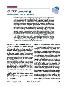
see
∑lz=k itz TEnd − TStart tk ≥ TStart ∧ il ≤ TEnd
avg(TStart , TEnd , uc) :=
(3)
So we can define the peak-to-avg ratio pta of a given usage characteristic uc (see equation 1) within a given analytical timeframe [TStart , TEnd ] in the following way: pta(TStart , TEnd , uc) :=
peak(TStart , TEnd , uc) avg(TStart , TEnd , uc)
(4)
In the following we will also use the average to peak ratio at p which is defined as the inverse of the pta: at p(TStart , TEnd , uc) :=
1 pta(TStart , TEnd , uc)
(5)
According to (Weinmann, 2011) we have to compare the costs of a classical dedicated approach with the costs of a cloud based approach. On the IaaS level it is common to be billed per service usage with a granularity of the atomic timeframe t level. Which
would be in case of Amazon Web Service that you are billed for a server instance per complete (or partial) hour usage. Let us name our dedicated costs per atomic timeframe d and our cloud costs per atomic timeframe c. Cloud costs c can be easily figured out because they are provided as pricing by their cloud service providers2 . Dedicated costs per atomic timeframe d are a little more complex to calculate. Nevertheless for estimations we can assume, that they can be defined via their amortizations. If a dedicated instance can be procured for p value units3 their dedicated costs per atomic timeframe can be calculated as follows4 : dAT F (p) =
p AT F
p (6) 3 · 365 · 24h p d5year (p) = 5 · 365 · 24h Typical amortization timeframes are a 3 year or a 5 year hardware regeneration interval (see equation 6). So a 500 $ server would have the following dedicated costs per atomic timeframe of 1h over a amortization interval of 3 years. d3year (p) =
500$ $ ≈ 0.019 (7) 3 · 365 · 24h h According to (Weinmann, 2011) the peak-to-average ratio pta should be greater than the relation between the variable costs per atomic timeframe c and the dedicated costs per atomic timeframe dAT F which can be expressed in the following form: c pta(TStart , TEnd , uc) > dAT F (p) ⇔ pta(TStart , TEnd , uc)dAT F (p) > c (8) dAT F (p) ⇔c< at p(TStart , TEnd , uc) In other words equation 4 provides a clear decision criteria to decide for or against a cloud based approach. By knowing your average to peak ratio at p,
your hardware procurement costs per instance p as well as your hardware amortization timeframes AT F (which is typically 3 or 5 years) it is possible to calculate a maximum of cloud costs per atomic timeframe cMAX until a cloud based approach is economical (see equation 9). Whenever a cloud service provider can realize instance pricings below cMAX we decide for a cloud based approach5 – in all other cases we should realize the system in a dedicated approach6 .
cMAX :=
dAT F (p) at p(TStart , TEnd , uc)
(9)
The at p function generates values between ]0.0...1.0[. Equation 9 shows us that low at p values – that means high peak to average relations (peaky usage scenarios) – will result into very high cMAX values. On the other side: High at p values – that means very low peak to average ratios (constant usage scenarios) – result into decreasing cMAX values. In the absolutely worst case of at p = 1.0 (absolutely constant usage) the dedicated costs become the maximum costs which means that the cloud service provider has to provide resources cheaper than the dedicated ones (which is very very unlikely).
d3year (500$) =
2 E.g. Amazon Web Services publishes these cloud costs per atomic timeframe here: http://aws.amazon.com/de/ec2/#pricing 3 E.g. US Dollars $ or Euro e 4 Be aware – this assumption do not account typical additional operational efforts like administration, cooling or electricity. Nevertheless we do not want to calculate exact costs we only want to know whether a cloud based approach is more economical than a dedicated one. In this case it is OK to give the dedicated side an advantage by not accounting aspects like administration, cooling, electricity, etc. although these costs are included in the variable costs on the cloud service provider side.
3
ANALYSED CASE STUDY
Table 1 shows all costs per group within the analysed timeframe. In total the L¨ubeck University of Applied Sciences had to spend 847.01$ in providing a (virtually) unlimited amount of server instances to 49 students organized in 9 groups within a timeframe of 13 calendar weeks. This sounds impressive but says in fact nothing about how cost efficient this performed cloud based approach was. Could we had reached the same results with a classical dedicated approach? Group WRSC 1 WRSC 2 WRSC 3 WRSC 4 GM 1 GM 2 GM 3 GM 4 GM 5
Size 5 6 4 6 6 6 6 5 5
Project WRSC Website WRSC Website WRSC Website WRSC Website Sailbot Tracking Sailbot Tracking Sailbot Tracking Sailbot Tracking Sailbot Tracking
Costs in $ 88.39$ 265.37$ 88.14$ 162.88$ 41.17$ 57.58$ 57.46$ 37.42$ 48.58$
Table 1: Group Overview
5 Only 6 Also
from an economical point of view. only from an economical point of view.
14
15
16
17
18
19
20
21
22
23
24
25
1.0 0.8 0.6 0.4 0.0
0 13
0.2
Avg to Max Box Usage Ratio
1500 1000
Processing Hours
500
50 30 20 0
10
Used Server Boxes
40
Average Box Usage Maximum Box Usage in an hour
(C) Average Box to Maximum Box Ratio according to Weinman
(B) Accumulated Processing Hours per Week
2000
(A) Maximum and Average Box Usage
13
14
15
16
17
Calendar Week
18
19
20
21
22
23
24
25
Calendar Week
14
16
18
20
22
24
Calendar Week
Figure 2: Analysed Box Usage
3.1
Usage Analysis
As we have found out in our analyzed use case – main cost driver was server/box usage. Thats why a detailed box usage analysis has been performed and is shown in figure 2. Figure 2(A) shows the maximum (according to equation 3) and average box usage (according to equation 2) per calendar week measured within the analysed timeframe (calendar week 13 - 25). Figure 2(B) shows the total sum of all processing hours generated by all used server boxes/instances per calendar week (this is the usage characteristic shown in equation 1 aggregated to calendar weeks). Figure 2(C) shows the average to peak load ratio (according to equation 5) per calendar week. Within the initial training phase (calendar week 13 - 21) the usage characteristic shows an extremely high maximum box usage but an astonishing low average usage. This characterizes an extreme peak load situation and results in extreme low at p ratios (see equation 5 and figure 2(C)). According to equation 8 or the definition of cMAX (equation 9) this shows a very ideal cloud computing (peaky) situation. So training phases seems to be very economical interesting cloud computing use cases. Within the project phase (calendar week 13 - 15) the usage characteristic shows dramatically reduced maximum as well as average box usages. Nevertheless the at p ratios (see equation 5 and figure 2(C)) stay in a very comfortable situation for cloud computing approaches. So we still have a peaky usage situation but on a dramatical lower level. So also development phases seems to be very economical interesting cloud computing use cases. The 24x7 phase (calendar week 21 - 24) shows raised maximum as well as average box usages (see figure 2(A). Also the at p ratios are raising within this phase – nevertheless the peaky usage remains but less distinctive. The 24x7 phase can be clearly seen in the accumulated processing hours (see figure 2(B)) which shows a clear peak in calendar weeks 22 - 24. We have stated already in section 3 that 24x7 seems to be
expensive and we can harden this conclusion by our usage analysis. This might surprise some readers. The migration phase (calendar week 25) was characterized by transferring the best solutions for the website and sailbot tracking service into the operational environment. Within this phase the systems run in a steady load scenario as can be seen in figure 2(A) (almost the same average box as well as maximum usage) and in figure 2(C) (an at p ratio near 1.0). According to equation 9 this shows an extreme uncomfortable situation for cloud computing situations – so steady loads seem to be no economical interesting cloud computing use cases.
3.2
Economical decision analysis
As we have seen in sections 3 and 3.1 we can identify different phases which are more cloud compatible than others from an ecomomical point of view. Training and development phases show very low at p ratios (see figure 2(C)) and therefore indicate peaky usage characteristics of resources which advantages cloud computing realizations7 (check equation 9). Other phases with less peaky usage characteristics (like our 24x7 or migration phase) disadvantage cloud computing realizations. So we have identified pro and cons for a cloud based realization of our educational labs. But how to decide? Now we are going to apply our decision model presented in section 2. Step 1: Determine the at p Ratio First of all we have to calculate our overall average to peak load ratio at p. According to equation 3 we have to define our timeframe basis (TEnd −TStart ). Our analysis timeframe covered the calendar weeks 13 25. So an intuitive timeframe for average building would be 13 weeks – but this implicates a continual usage of an educational lab over a complete year which is very uncommon. But in the university or college business educational labs are typically used one time per semester. In most cases an educational lab 7 From
an economical point of view.
1.74 ≈ 0.035 49 (11) 0.87 at p52w = ≈ 0.018 49 Step 2: Determine your dedicated costs First of all we have to find out how much would cost us a dedicated server. At the L¨ubeck University of Applied Sciences our procurement office could purchase the smallest possible server version8 for about 3055$. Equation 6 told us to calculate our dedicated costs per atomic timeframe (1h) in the following way for a 5 year amortization interval: at p26w =
3055$ $ ≈ 0.0697 (12) 5 · 365 · 24h h Step 3: Determine your maximal economical cloud costs Equation 9 told us to calculate our cMAX costs in the following way:
AWS Instance Type Micro Small (Standard) Large (Standard) XL (Standard) XL (High Memory) 2x XL (High Memory) 4x XL (High Memory) Medium (High CPU) XL (High CPU)
ECU