What-if Simulation Modeling in Business Intelligence - Semantic Scholar

International Journal of Data Warehousing and Mining, X(X), X-X, Oct-Dec 2008 1

What-if Simulation Modeling in Business Intelligence Matteo Golfarelli1 [email protected]

Stefano Rizzi1 [email protected]

DEIS - University of Bologna, Italy1 ABSTRACT Optimizing decisions has become a vital factor for companies. In order to be able to evaluate beforehand the impact of a decision, managers need reliable previsional systems. Though data warehouses enable analysis of past data, they are not capable of giving anticipations of future trends. What-if analysis fills this gap by enabling users to simulate and inspect the behavior of a complex system under some given hypotheses. A crucial issue in the design of what-if applications is to find an adequate formalism to conceptually express the underlying simulation model. In this paper we report on how, within the framework of a comprehensive design methodology, this can be accomplished by extending UML 2 with a set of stereotypes. Our proposal is centered on the use of activity diagrams enriched with object flows, aimed at expressing functional, dynamic, and static aspects in an integrated fashion. The paper is completed by examples taken from a real case study in the commercial area.

Keywords: What-if analysis, Business intelligence, Data warehouse, UML, Simulation.

1. Introduction Market conditions increasingly force companies to reduce waste and optimize decisions. This has become not only a critical, but a vital factor for companies. In this direction, business intelligence (BI) provides a set of tools and techniques that enable a company to transform its business data into timely and accurate information for the decisional process. BI platforms are used by decision makers to get a comprehensive knowledge of the business and of the factors that affect it, as well as to define and support their business strategies. The goal is to enable data-based decisions aimed at gaining competitive advantage, improving operative performance, responding more quickly to changes, increasing profitability and creating added value for a company (Rizzi, 2009a). As summarized by the so-called BI pyramid shown in Figure 1, BI platforms make it possible for companies to extract and process

their own business data and then transform those data into information useful for the decision-making process. The information obtained in this way is then contextualized and enhanced by the decision-makers’ own skills and experience, generating knowledge that is used to make conscious and well-informed decisions (Golfarelli & Rizzi, in press). The BI pyramid demonstrates that data warehouses, that have been playing a lead role within BI platforms in supporting the decision process over the last decade, are no more than the starting point for the application of more advanced techniques that aim at building a bridge to the real decision-making process. This is because data warehouses are aimed at enabling analysis of past data, but they are not capable of giving anticipations of future trends. Indeed, in order to be able to evaluate beforehand the impact of a strategic or tactical move, decision makers need reliable previsional systems. So, almost at the top of the BI pyramid, what-if analysis comes into play.

Copyright © 2008, Idea Group Inc. Copying or distributing in print or electronic forms without written permission of Idea Group Inc. is prohibited.

2 International Journal of Data Warehousing and Mining, X(X), X-X, Oct-Dec 2008

Figure 1. The business intelligence pyramid What-if analysis is a data-intensive simulation whose goal is to inspect the behavior of a complex system (i.e., the enterprise business or a part of it) under some given hypotheses called s c e n a r i o s . More pragmatically, what-if analysis measures how changes in a set of independent variables impact on a set of dependent variables with reference to a simulation model offering a simplified representation of the business, designed to display significant features of the business and tuned according to the historical enterprise data (Kellern et al., 1999). Example 1. A simple example of what-if query in the marketing domain is: How would my profits change if I run a 3×2 (pay 2, take 3) promotion for one week on all audio products on sale? Answering this query requires a simulation model to be built. This model, that must be capable of expressing the complex relationships between the business variables that determine the impact of promotions on product sales, is then run against the historical sale data in order to determine a reliable forecast for future sales. Among the killer applications for what-if analysis, it is worth mentioning profitability analysis in commerce, hazard analysis in finance, promotion analysis in marketing, and effectiveness analysis in production planning (Rizzi, 2009b). Less traditional, yet interesting applications described in the literature are urban and regional planning supported by spatial databases, index selection in relational databases, and ETL maintenance in data warehousing systems.

Surprisingly, though a few commercial tools are already capable of performing forecasting and what-if analysis, very few attempts have been made so far outside the simulation community to address methodological and modeling issues in this field (Golfarelli et al., 2006). On the other hand, facing a what-if project without the support of a design methodology is very time-consuming, and does not adequately protect designers and customers against the risk of failure. From this point of view, a crucial issue is to find an adequate formalism to conceptually express simulation models. Such formalism, by providing a set of diagrams that can be discussed and agreed upon with the users, could facilitate the transition from the requirements informally expressed by users to their implementation on the chosen platform. Besides, as stated by Balci (1995), it could positively affect the accuracy in formulating simulation problems and help the designer to detect errors as early as possible in the lifecycle of the project. Unfortunately, no suggestion to this end is given in the literature, and commercial tools do not offer any general modeling support. In this paper we show how, in the light of our experience with real case studies, an effective conceptual description of the simulation model for a what-if application in the context of BI can be accomplished by extending UML 2 with a set of stereotypes. As concerns static aspects we adopt as a reference the multidimensional model, used to describe both the source historical data and the prediction; the YAM2 (Abelló et al., 2006) UML extension for modeling multidimensional cubes is adopted to this end. From the functional and dynamic point of view, our proposal is centered on the use of activity diagrams enriched with object flows. In particular, while control flows allow sequential, concurrent, and alternative computations to be effectively represented, object flows are used to describe how business variables and cubes are transformed during simulation. The approach to simulation modeling proposed integrates and completes the design methodology presented by Golfarelli et al. (2006).



The paper is structured as follows. In the second section we survey the literature on modeling and design for what-if analysis. In the third section we outline the methodological framework that provides the context for our proposal. The fourth section enunciates a wish list for a conceptual formalism to support simulation modeling. The fifth section discusses how we employed UML 2 for simulation modeling. The sixth section proposes some examples taken from a case study concerning branch profitability and explains how we built the simulation model. Finally, the seventh section draws the conclusion.

2. Related Works and Tools There are a number of papers related to what-if analysis in the literature. In several cases, they just describe its applications in different fields such as e-commerce (Bhargava et al., 1997) hazard analysis (Baybutt, 2003), spatial databases (Klosterman, 1999; Lee & Gahegan, 2000), and index selection for relational databases (Chaudhuri & Narasayya, 1998). Other papers, such as the one by Fossett et al. (1991), are focused on the design of simulation experiments and the validation of simulation models. In (1999), Armstrong & Brodie survey a set of alternative approaches to forecasting, and give useful guidelines for selecting the best ones according to the availability and reliability of knowledge. In the literature about simulation, different formalisms for describing simulation models are used, ranging from colored Petri nets (Lee et al., 2006) to event graphs (Kotz et al., 1994) and flow charts (Atkinson & Shorrocks, 1981). The common trait of these formalisms is that they mainly represent the dynamic aspects of the simulation, almost completely neglecting the functional (how are data transformed during the simulation?) and static (what data are involved and how are they structured?) aspects that are so relevant for data-intensive simulations like those at the core of what-if analysis in BI. A few related works can be found in the database literature. Dang & Embury (2004) use constraint formulae to create hypothetical

scenarios for what-if analysis, while Koutsoukis et al. (1999) explore the relationships between what-if analysis and multidimensional modeling. Balmin et al. (2000) present the S E S A M E system for formulating and efficiently evaluating what-if queries on data warehouses; here, scenarios are defined as ordered sets of hypothetical modifications on multidimensional data. In all these papers, no emphasis is placed on modeling and design issues. In the context of data warehousing, there are relevant similarities between simulation modeling for what-if analysis and the modeling of ETL (Extraction, Transformation and Loading) applications; in fact, both ETL and what-if analysis can be seen as a combination of elemental processes each transforming an input data flow into an output. Vassiliadis et al. (2002) propose an ad hoc graphical formalism for conceptual modeling of ETL processes. While such proposal is not based on any standard formalisms, other proposals extend UML by explicitly modeling the typical ETL mechanisms. For example, Trujillo & LujanMora (2003) represent ETL processes by a class diagram where each operation (e.g., conversion, log, loader, merge) is modeled as a stereotyped class. All these proposals cannot be considered as feasible alternatives to ours, since the expressiveness they introduce is specifically oriented to ETL modeling. On the other hand, they strengthen our claim that extending UML is a promising direction for achieving a better support to the design activities in the area of BI. Finally, we mention two relevant approaches for UML-based multidimensional modeling (Abelló et al., 2006; , Lujan-Mora et al., 2006). Both define a UML profile for multidimensional modeling based on a set of specific stereotypes, and represent cubes at three different abstraction levels. However, the approach by Abelló et al. (2006) is preferred to the one by Lujan-Mora et al. (2006) for the purpose of this work since it allows for easily modeling different aggregation levels over the base cube, which is essential in simulation modeling for what-if analysis. Recently, what-if analysis has been gaining wide attention from vendors of business intelligence tools. For instance, both SAP



SEM-BPS (Strategic Enterprise Management Business Planning and Simulation) and SAS Forecast Server enable users to make assumptions on the enterprise state or future behavior, as well as to analyze the effects of such assumptions by relying on a wide set of forecasting models. Also Microsoft Analysis Services provides some limited support for what-if analysis. Other commercial tools that can be used for what-if analysis to some extent are Applix TM1, Powersim Studio and QlikView. Also spreadsheets and OLAP tools are often used to support what-if analysis. Spreadsheets offer an interactive and flexible environment for specifying scenarios, but lack seamless integration with the bulk of historical data. Conversely, OLAP tools lack the analytical capabilities of spreadsheets and are not optimized for scenario evaluation.

regression adopted for forecasting and the number of past years to be considered for regression. Distinguishing source variables among business variables is important since it enables the user to understand which are the “levers” that she can independently adjust to drive the simulation; also non-source business variables are involved in scenarios, where they can be used to store simulation results. Each scenario may give rise to different simulations, one for each assignment of values to the source variables and to the scenario parameters.

3. Methodological Framework As summarized in Figure 2, a what-if application is centered on a simulation model. The simulation model establishes a set of complex relationships between some business variables corresponding to significant entities in the business domain (e.g., products, branches, customers, costs, revenues, etc.). In order to simplify the specification of the simulation model and encourage its understanding by users, we functionally decompose it into scenarios, each describing one or more alternative ways to construct a p r e d i c t i o n of interest for the user. The prediction typically takes the form of a multidimensional cube, meant as a set of cells of a given type, whose dimensions and measures correspond to business variables, to be interactively explored by the user by means of an OLAP front-end. A scenario is characterized by a subset of business variables, called source variables, and by a set of additional parameters, called scenario parameters, whose value the user has to enter in order to execute the simulation model and obtain the prediction. While business variables are related to the business domain, scenario parameters convey information technically related to the simulation, such as the type of

Figure 2. What-if analysis at a glance Example 2. In the promotion domain of Example 1, the source variables for the scenario are the type of promotion, its duration, and the product category it is applied to; possible scenario parameters are the forecasting algorithm and its tuning parameters. The specific simulation expressed by the what-if query reported in the text is determined by giving values “3× 2”, “one week” and “audio”, respectively, to the three source variables. The prediction is a sales cube with dimensions W e e k and Product and measures Revenue, Cost and Profit, which the user could effectively analyze by means of any OLAP front-end. Designing a what-if application requires a methodological framework; the one we consider, presented by Golfarelli et al. (2006) and sketched in Figure 3, relies on the seven phases sketched in the following: 1. Goal analysis aims at determining which business phenomena are to be simulated, and how they will be characterized. The goals are expressed by (i) identifying the set of business variables users want to



Figure 3. A methodology for what-if analysis application design

2.

3.

4.

5.

6.

7.

monitor and their granularity; and (ii) outlining the relevant scenarios in terms of source variables users want to control. Business modeling builds a simplified model of the application domain in order to help the designer understand the business phenomenon, enable her to refine scenarios, and give her some preliminary indications about which aspects can be neglected or simplified for simulation. Data source analysis aims at understanding what information is available to drive the simulation, how it is structured and how it has been physically deployed, with particular regard to the cube(s) that store historical data. Multidimensional modeling structurally describes the prediction by taking into account the static part of the business model produced at phase 2 and respecting the requirements expressed at phase 1. Very often, the structure of the prediction is a coarse-grain view of the historical cube(s). Simulation modeling defines, based on the business model, the simulation model allowing the prediction to be constructed, for each given scenario, from the source data available. Data design and implementation, during which the cube type of the prediction and the simulation model are implemented on the chosen platform, to create a prototype for testing. Validation evaluates, together with the users, how faithful the simulation model is to the real business model and how reliable the

prediction is. If the approximation introduced by the simulation model is considered to be unacceptable, phases 4 to 7 are iterated to produce a new prototype. The five analysis/modeling phases (1 to 5) require a supporting formalism. Standard UML can be used for phases 1 (use case diagrams), 2 (a class diagram coupled with activity and state diagrams) and 3 (class, component and deployment diagrams), while any formalism for conceptual modeling of multidimensional databases can be effectively adopted for phase 4 (e.g., (Abelló et al., 2006) or (Lujan-Mora et al., 2006)). On the other hand, finding in the literature a suitable formalism to give broad conceptual support to phase 5 is much harder.

4. A Wish List for Simulation Phase 5, simulation modeling, is the core phase of design. In the light of our experience with real case studies of what-if analysis in the BI context, we enunciate a wish list for a conceptual formalism to support it: # 1 The formalism should be capable of coherently expressing the simulation model according to three perspectives: functional, that describes how business variables are transformed and derived from each other during simulation; dynamic, required to define the simulation workflow in terms of sequential, concurrent and alternative tasks; static, to explicitly represent how business variables are aggregated during simulation.



#2 It should provide constructs for expressing the specific concepts of what-if analysis, such as business variables, scenario parameters, predictions, etc. # 3 It should support hierarchical decomposition, in order to provide multiple views of the simulation model at different levels of abstraction. #4 It should be extensible so that designers can effectively model the peculiarities of the specific application domain they are describing. # 5 It should be easy to understand, to encourage the dialogue between designers and final users. # 6 It should rely on a standard notation to minimize the learning effort. UML perfectly fits requirements #4 and #6, and requirement #5 to some extent. In particular, it is well known that the stereotyping mechanism allows UML to be easily extended. As to requirements #1 and #3, the UML diagrams that best achieve integration of functional, dynamic and static aspects while allowing hierarchical decomposition are activity diagrams. Within UML 2, activity diagrams take a new semantics inspired by Petri nets, which makes them more flexible and precise than in UML 1 (OMG, 2008). Their most relevant features for the purpose of this work are summarized below: • An activity is a graph of activity nodes (that can be action, control or object nodes) connected by activity edges (either control flows or object flows). • An action node represents a task within an activity; it can be decorated by the rake symbol to denote that the action is described by a more detailed activity diagram. • A control node manages the control flow within an activity; control nodes for modeling decision points, fork and synchronization points are provided. • An object node denotes that one or more instances of a given class are available within an activity, possibly in a given state. Input and output objects for activities are denoted by overlapping them to the activity borderline.

Control flows connect action nodes and control nodes; they are used to denote the flow of control within the activity. • Object flows connect action nodes to object nodes and vice versa; they are used to denote that objects are produced or consumed by tasks. • Selection and transformation behaviors can be applied to object nodes and flows to express selection and projection queries on object flows. Though activity diagrams are a nice starting point for simulation modeling since they already support advanced functional and dynamic modeling, some extensions are required in order to attain the desired expressiveness as suggested by requirement #2. In particular, it is necessary to define an extension allowing basic multidimensional modeling of objects in order to express how simulation activities are performed on data at different levels of aggregation. With regard to this we recall that, as stated by OMG (2008), it is expected that the UML 2 Diagram Interchange specification will support a form of integration between activity and class diagrams, by allowing an object node to be linked to a class diagram that shows the classifier for that object and its relations to other elements. In this way, while activities provide a functional view of processes, associated class diagrams can be used to show static details. This argument has a relevant weight in our approach, since we associate activity diagrams with class diagrams to basically model the structure of cubes and their relationships with business variables. •

5. Expressing Simulation Models in UML 2 In our proposal, the core of simulation modeling is a set of UML 2 diagrams organized as follows: 1. A use case diagram that reports a what-if analysis use case including one or more scenario use cases. 2. One or more class diagrams that statically represent scenarios and multidimensional cubes. A scenario is a class whose attributes are scenario parameters; it is related via an



aggregation to the business variables that act as source variables for the scenario. Cubes are represented in terms of their dimensions, levels and measures. 3. An activity diagram (called s c e n a r i o diagram) for each scenario use case. Each scenario diagram is hierarchically exploded into activity diagrams at increasing level of detail. All activity diagrams represent, as object nodes, the business variables, the scenario parameters and the cubes that are produced and consumed by tasks.

5.1. Static Modeling

its source variables) name: base class: icon: description: tagged values:

business variable class B classes of this stereotype represent business variables isNumerical (type Boolean, indicates whether the business variable can be used as a measure) i s D i s c r e t e (type Boolean, indicates whether the business variable can be used as a dimensions)

Representation of cubes is supported by YAM2 (Abelló et al., 2006), a UML extension for conceptual multidimensional modeling. YAM2 name: scenario parameter models concepts at three different detail levels: icon: SP upper, intermediate, and lower. At the upper base class: attribute level, stars are described in terms of facts and description: attributes of this stereotype dimensions. At the intermediate level, a fact is represent parameters that model exploded into cells at different aggregation user settings concerning granularities, and the aggregation levels for scenarios each dimension are shown. Finally, at the lower constraints: a scenario parameter attribute level, measures of cells and descriptors of belongs to a scenario class levels are represented. In our approach, the intermediate and lower levels are considered. The intermediate level is 5.1. Dynamic Modeling used to model, through the «cell» stereotype As already mentioned, activity diagrams at (represented by the C icon), the aggregation different levels of detail are used to granularities at which data are processed by dynamically model how simulation is carried activities, and to show the combinations of out. The main features of this representation are dimension levels («level» stereotype, summarized below: represented by the L icon) that define those • The rake symbol denotes the actions that granularities. The lower level allows single will be further detailed in subdiagrams. measures of cells to be described as attributes • Object nodes that represent cubes of class of cells, and their type to be separately modeled cells are named as Cube of through the «KindOfMeasure» stereotype. . The state in the object node is In order to effectively use YAM2 for used to express the current state of the simulation modeling, three additional cubes being processed. stereotypes are introduced for modeling, • Other object nodes represent business respectively, scenarios, business variables and variables and scenario parameters used by scenario parameters: activities. name: scenario • The «datastore» stereotype is used to base class: class represent an object node that stores nonicon: S transient information, such as a cube storing description: classes of this stereotype historical data. represent scenarios • Selection operations on cubes are constraints: a s c e n a r i o class is an represented by decorating object flows with aggregation of b u s i n e s s a selection behavior («selection» variable classes (that represent its source Copyright © 2007, Idea variables) Group Inc. Copying or distributing in print or electronic forms without written permission of Idea Group Inc. is prohibited.


stereotype). Projection operations on cubes (i.e., restricting the set of measures to be processed) are represented by decorating object flows with a transformation behavior («transformation» stereotype). Based on the characteristics of each specific application domain, some ad hoc stereotypes can be defined to model recurrent types of actions. The action stereotypes we defined based on our experience are listed below: name: olap base class: action description: actions of this stereotype transform cubes by applying OLAP operators; mainly, they aggregate, select and project cube cells constraints: at least one input and one output object flow must connect an olap action to Cube of object nodes name: base class: description: constraints:

name: base class: description:

constraints:

name: base class: description:

regression action actions of this stereotype carry out regression to extrapolate future data from past data at least one input object flow and one output object flow must connect a regression action to Cube of object nodes apportion action actions of this stereotype apportion values of aggregate cube cells among a set of finer cube cells according to a given driver at least one input object flow and one output object flow must connect a regression action to Cube of object nodes user input action actions of this stereotype allow manual input of data

constraints:

at least one output object flow must exit a user input action

6. A Case Study Orogel S.p.A. is a large Italian company in the area of deep-frozen food. It has a number of branches scattered on the national territory, each typically entrusted with selling and/or distribution of products. Its data warehouse includes a number of data marts, one of which dedicated to commercial analysis and centered on a sales cube with dimensions M o n t h , Product, Customer, and Branch. The managers of Orogel are willing to carry out an in-depth analysis on the profitability (i.e., the net revenue) of branches. More precisely, they wish to know if, and to what extent, it is convenient for a given branch to invest on either selling or distribution, with particular regard to the possibility of taking new customers or new products. Thus, the four scenarios chosen for prototyping are: (i) analyze profitability during next 12 months in case one or more new products were taken/dropped by a branch; and (ii) analyze profitability during next 12 months in case one or more new customers were taken/dropped by a branch. Decision makers ask for analyzing profitability at different levels of detail; the finest granularity required for the prediction is the same of the sales cube. The main issue in simulation modeling is to achieve a good compromise between reliability and complexity. To this end, in constructing the simulation model we adopted a two-step approach that consists in first forecasting past data, then “stirring” the forecasted data according to the event (new product or new customer) expressed by the scenarios. We mainly adopted statistical techniques for both the forecasting and the stirring steps; in particular, linear regression is employed to forecast unit prices, quantities and costs starting from historical data taken from the commercial data mart and from the profit and loss account during a past period taken as a reference. Based on the decision makers’ experience, and aimed at avoiding irrelevant statistical fluctuations



Sales decision support Monthly reporting on revenues Sales manager OLAP analysis of budget variance

Management controller

What -if analysis of profitability General manager

«include»

«include»

«include»«include»

Add product

Remove product

Sales agent

Branch manager

Add customer

Remove customer

Figure 4. Use-case diagram «KindOfMeasure»

Cost

{isNumerical}

YearlyQuantity C

«KindOfMeasure»

Quantity B

quantitySold:Quantity

{isNumerical}

EconomicCategory {isDiscrete} BL

Year {isDiscrete}

Branch {isDiscrete}

BL

Product {isDiscrete}

BL

Customer {isDiscrete}

BL

Sale

unitPrice*quantitySoldfixedCosts- variableCosts

B

Month {isDiscrete}

BL

BL

C

quantitySold:Quantity unitPrice:Price fixedCosts:Cost variableCosts:Cost /netRevenue:Revenue

CostElement {isDiscrete} BL

Profit&LossAccount C costValue:Cost

Figure 5. Multidimensional class diagram while capturing significant trends, we adopted different granularities for forecasting the different measures of the prediction cube (Golfarelli, 2006).

6.1. Representing the Simulation Model: Static Aspects The four what-if use cases (one for each scenario) are part of a use case diagram that, as suggested by List et al. (2000), expresses how the different organization roles take advantage of BI in the context of sales analysis. Figure 4

shows a part of the use-case diagram for our case study. For space reasons, in this paper we will discuss only the Add product use case. The class diagram shown in Figure 5 gives a (partial) specification of the multidimensional structure of the cubes involved. Sale is the base cell of the sales cube; its measures are q u a n t i t y S o l d , u n i t P r i c e , fixedCosts, variableCosts and netRevenue (the latter is derived from the others), while the dimensions are Product, Customer, Month and Branch. Aggregations from one level to another



referenceBranch toBranch

AddProduct

S

SPregressionLength:Integer SPforecastTechnique:String

UnitPriceScaling Branch {isDiscrete}

B

QtyScaling B

BL Product {isDiscrete}

BL

Figure 6. Scenario class diagram What -if analysis of profitability

stored in the data warehouse

«datastore»

Scenario management

Cube of Sale [forecast]

Cube of Sale [history] stored in

Stir product

Forecast

«datastore»

«datastore»

Cube of Profit&LossAccount [history]

Cube of Sale [prediction]

Figure 7. Scenario diagram Scenario management

UnitPriceScaling

«userInput»

Input parameters

«userInput»

Input source variables

Product

Branch

AddProduct QtyScaling

Figure 8. Activity diagram for Scenario management represent roll-up hierarchies (e.g., products roll up to economic categories). Both dimension levels and measure types are further stereotyped as business variables. YearlyQuantity is a cell derived from Sale by aggregating by EconomicCategory, Year and

Branch and projecting on quantitySold; it will be used in activity diagrams to model aggregated data for regression. Finally, the Profit&LossAccount base cell stores the costs by Year, CostElement and Branch.



Figure 6 reports an additional class diagram that statically represents the AddProduct scenario in terms of its parameters and source variables: • forecastTechnique and regressionLength are scenario parameters. The first one specifies if forecast should be based on regression (which means that trends for the future are extrapolated from past data) or on judgment (which means that trends for the future are manually entered by users). The second one stores the number of past years to be used as input for regression. • Among source variables, AddProduct.addedProduct is the specific product that users may decide to add to a branch, while AddProduct.toBranch is the specific branch that product is added to. AddProduct.referenceBranch is a branch, that already sells AddProduct.addedProduct, and that users choose as a reference for estimating quantities and unit prices for selling A d d P r o d u c t . a d d e d P r o d u c t in A d d P r o d u c t . t o B r a n c h . Finally, UnitPriceScaling and QtyScaling store the percentage change in unit price and quantity sold that users expect in AddProduct.toBranch with reference to AddProduct.referenceBranch.

6.2. Representing the Simulation Model: Dynamic Aspects The Add product use case is expanded in the scenario diagram reported in Figure 7, that provides a high-level overview of the whole simulation process. The S c e n a r i o management action is aimed at entering values for the scenario parameters and the source variables. The cube storing historical sales data is represented as an object node called Cube of Sale , with state [history] and stereotyped as «datastore». The Forecast action takes this cube and the cube storing the profit and loss account, and produces in output a Cube of Sale with state [forecast] storing the sales trends for next year. This cube is then transformed by the Stir product action, that simulated the addition of a product to a branch,

to produce the final prediction in the form of a Cube of Sale with state [prediction]. The action nodes of the context diagram are exploded into a set of hierarchical activity diagrams whose level of abstraction may be pushed down to describing tasks that can be regarded as atomic. Some of them are reported here in a simplified form and briefly discussed below: • Activity Scenario management (Figure 8) enables users to set all source variables and scenario parameters. This is represented by decorating actions with the « u s e r input» stereotype. • Activity Forecast (Figure 9) is aimed at extrapolating sale data for the next twelve months, represented by the Cube of Sale object node with state [forecast]. This is done separately for each single measure of the Sale cell. In particular, forecasting general costs requires to extrapolate the future fixed and variable costs from the past profit and loss accounts, and scale variable costs based on the forecasted quantities. Input and output objects nodes for Forecast are emphasized by placing them on the activity borderline. The «selection» and «transformation» stereotypes are used to express, respectively, that only the sales data of the last few years have to be selected (as defined by the regressionLength scenario parameter) and which measure(s) from cube cells are to be processed. States [ g c F o r e c a s t ] , [qtyForecast] and [upForecast] denote forecast cubes where only cost, quantity and price measures have been calculated, respectively. These three cubes are then joined together through the Drill-across action. • The quantity forecast granularity suggested by users is Y e a r , Branch, EconomicCategory. The forecast for next year (Figure 10) can be done, depending on the value taken by the forecastTechnique scenario parameter, either by judgment (the yearly quantities for next year are directly entered by the user) or by regression (based on the yearly quantities sold during the last regressionLength years, stored in a Cube of YearlyQuantity with state [history]). In



«datastore»

Cube of Sale [history]

Forecast «selection» last AddProduct.regressionLength years



«transformation» Sale.fixedCosts, Sale.variableCosts

«transformation» Sale.quantitySold

«datastore»

«transformation» Sale.unitPrice

Forecast quantity

Cube of Profit&LossAccount [history] Forecast general costs

general costs for next 12 months


Cube of Sale [qtyForecast]


Cube of Sale [gcForecast]

Forecast unit price

quantitiesfor next 12 months


unit prices for next 12 months

Cube of Sale [upForecast]


Figure 9. Activity diagram for Forecast

•

both cases, the total quantities by branch and economic category are stored in a Cube of YearlyQuantity with state [forecast]. This cube is then apportioned on the single months, products and customers proportionally to the quantities sold during the last 12 months. Note the use of names to express specific roles of object flows within actions. For instance, the time span object flow in input to Quantity regression carries the temporal span used for regression; the driver object flow in input to Quantity apportion denotes the flow carrying the cube whose cells provide the historical data used as a driver to proportionally distribute yearly quantities among months, products and customers. Finally, Figure 11 explodes the S t i r product activity, that simulates the effects of adding a new product

(AddProduct.addedProduct) to a branch (AddProduct.toBranch) by reproducing the sales of that product in a different branch (AddProduct.referenceBranch) where that product is already sold. First, the past sales of the product are scaled according to the user-specified percentages stored in the q t y S c a l i n g and unitPriceScaling source variables (action Scale quantities and unit prices ), and they are ascribed to the AddProduct.toBranch branch. This action produces a Cube of Sale object node with state [ a d d e d P r o d u c t ] . Then, cannibalizationi on forecasted sales for the other products (Cube of Sale with state [forecast]) is simulated by applying a product correlation matrix (Cube of C o r r e l a t i o n ) built by judgmental techniques, i.e., by user input. Finally, fixed costs are properly redistributed on the



«datastore»


Forecast quantity

Cube of Sale [history] [AddProduct.forecastTechnique ='regression']

«selection» last 12 months

«olap»

Group by Year, Branch, Econ.Cat.

«transformation» AddProduct.regressionLength

Cube of YearlyQuantity [history]

«length»

AddProduct

«history» «regression»

Quantity regression


quantities for next year «userInput»

Cube of YearlyQuantity [forecast]

Input yearly quantities

«apportion»

Quantity apportion by Month, Product, Customer

«driver»

quantitiesfor next 12 months


Figure 10. Activity diagram for Forecast quantity single forecasted sales, changing the state of the Cube of Sale object node from [cannibalized] to [prediction].

6.3. Building the Simulation Model In this section we give an overview of the approach we pursued to build the UML simulation model for Orogel. The starting points are the use case diagram, the business model and the multidimensional model obtained, respectively, from phases 1, 2 and 4 of the methodology outlined in the third section. For simplicity, we assume that the multidimensional model is already coded in YAM2. 1. The class diagram is created first, by extending the multidimensional model that describes the prediction with the static specification of scenarios, source variables and scenario parameters. 2. For each scenario reported in the use case diagram, a high-level scenario diagram is

created. This diagram should show the macro-phases of simulation, the main data sources and the prediction. The object nodes should be named consistently with the classes diagram. 3. Each activity in each scenario diagram is iteratively exploded and refined into additional activity diagrams. As new, more detailed activities emerge, business variables and scenario parameters from the class diagram may be included in activity diagrams. Relevant aggregation levels for processing business variables within activities may be identified, in which case they are increasingly reported on the class diagram. Refinement goes on until the activities are found that are elemental enough to be understood by an executive designer/programmer. We chose to build activity diagrams in a topdown fashion since, in our experience, this approach provides a stronger thread for



Stir product QtyScaling

«selection» Sale.Product=AddProduct.addedProduct AND Sale.Branch=AddProduct.referenceBranch

«scalingfactor» «userInput»

«scale»

Input correlations

Scale quantities and unit prices

Cube of Correlation

Cube of Sale [addedProduct]

Cannibalize

Cube of Sale [forecast] «scalingfactor»

UnitPriceScaling



Cube of Sale [cannibalized]

Distribute fixed costs

«datastore»

Cube of Sale [prediction]

Figure 11. Activity diagram for Stir product reasoning with users, especially in the very common case that, in the beginning, users have little or no idea about how the basic laws that rule their business world should be coded. In order to validate the simulation model, we used 2003 and 2004 data to forecast the profitability for 2005. A comparison with the actual data for 2005 yielded an average error of about 18% on the total profitability of the single branches, which decision makers judged to be very promising. The error on the total profitability for 2005 was significantly lower (about 7%) due to a compensation effect.

7. Conclusion To sum up, our approach to simulation modeling fulfills the wish list proposed in the fourth section as follows: (#1) Static, functional and dynamic aspects are modeled in an integrated fashion by combining use case, class and activity diagrams; (#2) Specific constructs of what-if analysis are modeled through the UML stereotyping mechanism; (#3) Multiple

levels of abstraction are provided by both activity diagrams, through hierarchical decomposition, and class diagrams, through the three detail levels provided by YAM2; (#4) Extensibility is provided by applying the stereotyping mechanism; (#5) Though completely understanding the implications of a UML diagram is not always easy for business users, the precision and methodological rigor encouraged by UML let them more fruitfully interact with designers, thus allowing solutions to simulation problems to emerge easily and clearly during analysis even when, in the beginning, users have little or no idea about how the basic laws that rule their business world should be coded; (#6) UML is a standard. In practice, the approach proved successful in making the design process fast, wellstructured and transparent. A critical evaluation of the proposed approach against its possible alternatives unveils that the decisive factor is the choice of adopting UML as the modeling language rather than devising an ad hoc formalism. Indeed, adopting UML poses some



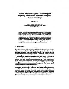
Figure 12. Scenario management window for defining hypotheses on general costs constraints in the syntax of diagrams (for instance, the difficulty of directly showing on activity diagrams the aggregation level at which cells are processed); on the other hand it brings some undoubted advantages to the designer, namely, the fact of relying on a standard and widespread formalism. Besides, using hierarchical decomposition of activity diagrams to break down the complexity of modeling increases the scalability of the approach. The simulation model designed has been prototyped in C#. Oracle 9i is the platform chosen for hosting the predictions and as a repository for business variables and model parameters. Business Objects is used for OLAP analysis of predictions. A screenshot of the GUI used to input business variables and scenario parameters is reported in Figure 12; in particular, the form used to formulate hypotheses about general costs is shown. We conclude by remarking that the proposed formalism is oriented to support simulation modeling at the conceptual level, which in our opinion will play a crucial role in reducing the overall effort for design and in simplifying its reuse and maintenance. Devising a formalism capable of adequately expressing the simulation model at the logical level, so that it can be directly translated into an implementation, is a subject for our future work.

REFERENCES Abelló, A., Samos, J., & Saltor F. (2006). YAM2: a multidimensional conceptual model extending UML. Information Systems, 31(6), 541-567. Armstrong, S., & Brodie, R. (1999). Forecasting for marketing. In G. Hooley and M. Hussey (Eds.), Quantitative methods in marketing (pp. 92-119). Int. Thompson Business Press. Atkinson, W. D., & Shorrocks, B. (1981). Competition on a Divided and Ephemeral Resource: A Simulation Model. Journal of Animal Ecology, 50, 461-471. Baybutt, P. (2003). Major hazards analysis – An improved process hazard analysis method. Process Safety Progress, 22(1), 21-26. Balci, O. (1995). Principles and Techniques of Simulation Validation, Verification, and Testing. In Proceedings Winter Simulation Conference (pp. 147-154). Arlington, USA. Balmin, A., Papadimitriou, T., & Papakonstantinou, Y. (2000). Hypothetical Queries in an OLAP Environment. In Proceedings Conference on Very Large Data Bases (pp. 242-253). Cairo, Egypt. Bhargava, H. K., Krishnan, R., & Muller, R. (1997). Electronic Commerce in Decision Technologies: A Business Cycle Analysis. International Journal of Electronic Commerce, 1(4), 109-127. Chaudhuri, S., & Narasayya, V. (1998). AutoAdmin what-if index analysis utility. SIGMOD Records, 27(2), 367-378. Dang, L., & Embury, S. M. (2004). What-If Analysis with Constraint Databases. In Proceedings British National Conference on Databases. Edinburgh, Scotland. Fossett, C., Harrison, D., & Weintrob, H. (1991). An assessment procedure for simulation models: a case study. Operations Research, 39(5), 710-723.



Golfarelli, M., Rizzi, S., & Proli, A. (2006). Designing What-if Analysis: Towards a Methodology. In Proceedings International Workshop on Data Warehousing and OLAP (pp. 51-58). Arlington, USA. Golfarelli, M., & Rizzi, S. (in press). Data warehouse design: Modern principles & methodology. McGraw-Hill Professional. Kellner, M., Madachy, R., & Raffo, D. (1999). Software process simulation modeling: Why? What? How? Journal of Systems and Software, 46(2-3), 91-105. Klosterman, R. (1999). The What if? collaborative support system. Environment and Planning, B: Planning and Design, 26, 393-408. Kotz, D., Toh, S. B., & Radhakrishnan, S. (1994). A Detailed Simulation Model of the HP 97560 Disk Drive (Tech. Rep.). Hanover, USA: Dartmouth College. Koutsoukis, N. S., Mitra, G., & Lucas, C. (1999). Adapting on-line analytical processing for decision modelling: the interaction of information and decision technologies. Decision Support Systems, 26(1), 1-30. Lee, C., Huang, H. C., Liu, B., & Xu, Z. (2006). Development of timed colour Petri net simulation models for air cargo terminal operations. Computers and Industrial Engineering, 51(1), 102-110. Lee, I., & Gahegan, M. (2000). What-if Analysis for Point Data Sets Using Generalised Voronoi Diagrams. In Proceedings International Conference on GeoComputation. Greenwich, UK. List, B., Schiefer, J., & Tjoa, A. M. (2000). ProcessOriented Requirement Analysis Supporting the Data Warehouse Design Process – A Use Case Driven Approach. Proceedings 11th International Conference Database and Expert Systems Applications (pp. 593-603). London, UK. Lujan-Mora, S., Trujillo, J., & Song, I.-Y. (2006). A UML profile for multidimensional modeling in data warehouses. Data & and Knowledge Engineering, 59(3), 725-769. OMG, (2008). UML: Superstructure, version 2.0. Retrieved December 10, 2008, from http:// www.omg.org. Rizzi, S. (2009a). Business Intelligence. In L. Liu and T. Özsu (Eds.), Encyclopedia of Database Systems. Springer. Rizzi, S. (2009b). What-if analysis. In L. Liu and T. Özsu (Eds.), Encyclopedia of Database Systems. Springer. Trujillo, J., & Lujan-Mora, S. (2003). A UML based approach for modelling ETL processes in data warehouses. In Proceedings International Conference on Conceptual Modeling (pp. 307-320). Chicago, USA. Vassiliadis, P., Simitsis, A., & Skiadopoulos, S. (2002). Conceptual modeling for ETL processes. In Proceedings International Workshop on Data Warehousing and OLAP (pp. 14-21). McLean, USA.

i

Cannibalization is the process by which a new product gains sales by diverting sales from existing products, which may deeply impact the overall profitability.


What-if Simulation Modeling in Business Intelligence - Semantic Scholar

What-if Simulation Modeling in Business Intelligence - Semantic Scholar

Suggest Documents

modeling business - Semantic Scholar

Business Process Intelligence - Semantic Scholar

Business Intelligence in Blogs: Understanding ... - Semantic Scholar

Business Intelligence in Collaborative Networks - Semantic Scholar

Simulation Modeling in Botanical Epidemiology ... - Semantic Scholar

Simulation Modeling in Botanical Epidemiology ... - Semantic Scholar

Perspectives in Modeling: Simulation, Database ... - Semantic Scholar

Business Intelligence Modeling in Launch Operations - Intelligent ...

Business Intelligence Modeling in Launch Operations - Intelligent

Modeling Business Strategy - Semantic Scholar

Business Intelligence and the Web - Semantic Scholar

Behavioural Business Intelligence Framework ... - Semantic Scholar

Business Process Intelligence : Discovering and ... - Semantic Scholar

Usability evaluation for Business Intelligence ... - Semantic Scholar

Situational Business Intelligence 1. Introduction - Semantic Scholar

Real-time Business Intelligence System ... - Semantic Scholar

9 Collaborative Business Intelligence - Semantic Scholar

Towards business intelligence systems success - Semantic Scholar

SOLAP technology: Merging business intelligence ... - Semantic Scholar

Real-time Business Intelligence System ... - Semantic Scholar

Modeling, Simulation, and Optimization of ... - Semantic Scholar

Modeling and Simulation Approaches for ... - Semantic Scholar

fundamentals of simulation modeling - Semantic Scholar

Three-dimensional Modeling, Simulation and ... - Semantic Scholar