sites of interest to a nearby rock site that is considered a "reference" motion. ... study show that surface-rock sites can have a site response of their own, which ...
Bulletin of the Seismological Society of America, Vol. 86, No. 6, pp, 1733-1748, December 1996
What Is a Reference Site? by Jamison H. Steidl, Alexei G. Tumarkin, and Ralph J. Archuleta
Abstract
Many methods for estimating site response compare ground motions at sites of interest to a nearby rock site that is considered a "reference" motion. The critical assumption in these methods is that the surface-rock-site record (reference) is equivalent to the input motion at the base of the soil layers. Data collected in this study show that surface-rock sites can have a site response of their own, which could lead to an underestimation of the seismic hazard when these sites are used as reference sites. Data were collected from local and regional earthquakes on digital recorders, both at the surface and in boreholes, at two rock sites and one basin site in the San Jacinto mountains, southern California. The two rock sites, Keenwild and Pifion Flat, are located on granitic bedrock of the southern California peninsular ranges batholith. The basin site, Garner Valley, is an ancestral lake bed with watersaturated sediments, on top of a section of decomposed granite, which overlies the competent bedrock. Ground motion is recorded simultaneously at the surface and in the bedrock at all three sites. When the surface-rock sites are used as the reference site, i.e., the surface-rock motion is used as the input to the basin, the computed amplification underestimates the actual amplification at the basin site for frequencies above 2 to 5 Hz. This underestimation, by a factor of 2 to 4 depending on frequency and site, results from the rock sites having a site response of their own above the 2to 5-Hz frequencies. The near-surface weathering and cracking of the bedrock affects the recorded ground motions at frequencies of engineering interest, even at sites that appear to be located on competent crystalline rock. The bedrock borehole ground motion can be used as the reference motion, but the effect of the downgoing wave field and the resulting destructive interference must be considered. This destructive interference may produce pseudo-resonances in the spectral amplification estimates. If one is careful, the bedrock borehole ground motion can be considered a good reference site for seismic hazard analysis even at distances as large as 20 km from the soil site.
Introduction It has long been known that each soil type responds differently when subjected to ground motion from earthquakes. Usually, the younger, softer soils amplify ground motion relative to older, more competent soils or bedrock. One of the goals of engineering seismology has been to try to quantitatively measure this amplification of ground motion throughout metropolitan regions in earthquake-prone areas. These measurements can then be used to help distinguish regions where the seismic hazard is greatest due to amplification from the surface geology and subsurface structure. The varied damage patterns seen over small distances in the wake of large earthquakes is easily understood when we look at the variation over small distances in recorded ground motion. As an example, two stations located only 120 m from each other on identical soil, with fiat topogra-
phy, show a distinct variability in their records of ground motion from the same M4.7 Landers, California, aftershock (Fig. la). A second example shows ground motion recorded at two rock sites located 150 m from each other for the same event (Fig. lb). These examples were recorded during the 1992 Landers, California, aftershock sequence in the epicentral region of the Landers mainsbock (Steidl, 1993). Although these sites appear to have a common long-period signal, the variability at higher frequencies is clear. A common factor in many of the methods for estimating amplification of ground motion at a particular site due to its near-surface geology is to use a nearby bedrock site as the reference motion. The critical assumption in these methods is that the surface-rock-site record (reference) is equivalent to the input motion at the base of the soil layers. Here we define a reference as a site that has a fiat transfer function
1733
1734
J.H. Steidl, A. G. Tumarkin, and R. J. Archuleta
a) Assumption: Surface Bedrock Site = Input to Base of Soil Site
UCSB Dense Array M4.3 Landers Aftershoek, 7 July 1992
Two Soil Sensors
~ ] I I Scale0.075g
622Ea~t-I~est
619East-West
'tilt' 'r
~
~
-
-
622North-S0uth
8
I0
12 14 Time [s]
"Reference" Site?
Soil Sites
~
SI9 North-South
16
g
10
12 14 Time [s]
,
16
P~t~~~o~rce I
\
\
Figure 2. Schematic diagram showing the common assumption that surface bedrock sites are considered the reference motion to nearby soil sites.
b) UCS[I Dense Array M4.3 Landers Aftershoek, 7 July 1992
TwoRockSensors
t
623North-South
6
8
10
12
Time Is]
14
16
621East-West
621 North-South
8
10
12
14
16
1~
Time [s]
Figure 1. Variation of ground motion seen in three-component data recorded from an M4.3 aftershock following the 1992 M7.3 Landers, California, earthquake at the UCSB dense array of portable accelerometers. (a) Two soil sites separated by 120 m. (b) Two rock sites separated by 150 m.
with an amplitude of one, i.e., a half-space response; it behaves like the bedrock below the soil layers, with the exception of the free-surface effect. Given that the input motion below the soil layers is not usually known, for practical reasons, seismologists will use the nearby rock site and make this assumption. Figure 2 is a schematic diagram that illustrates this assumption. How similar is the motion at the base of the soil layers and the bedrock outcrop 1 km away or 5 km away? Previous studies have shown variability in surface ground motion over small distances at both soil and rock sites (Cranswick, 1988; Menke et al., 1990; Vernon et al., 1991; Schneider et al., 1992; Steidl, 1993). This variability, especially at rock sites, suggests that this basic assumption may break down above a site-dependent frequency. We define site response here in three ways. First, we
use a theoretical definition, by which an input motion at the base of a soil column is propagated up through the soils to estimate the site response. The filter that must be applied to the incident wave to obtain the surface motion is the theoretical site response and is used extensively in engineering seismology and seismic hazard analysis. Second, we use a practical definition, the modifications to motions on rock at the surface needed to get motions on soil at the surface. This estimate, usually in the form of spectral ratios of soil to rock, is widely used by seismologists. Third is a borehole definition, the difference between motions recorded in a bedrock borehole and motions recorded at the surface. Each of these site-response estimates is used in this study. In an attempt to understand the variability in our reference sites, we will compare data from a series of borehole sensors located along the San Jacinto fault zone in southern California with the hope of addressing some of the following questions. Is this variability only at the surface or does it exist at depth? How much of the variability seen at closely spaced rock sites is due to weathering of the rock at the surface? How similar are borehole rock records compared to surface rock records? How similar are borehole recordings separated by 5 km or even 20 km? Is the bedrock borehole recording a better reference for site-response studies? The results will be presented by first showing the empirical estimation of site response at the Garner Valley site. A borehole sensor located below the soil column in competent granitic rock is used as the denominator in Fourier spectral ratio estimates of amplification. We will also compare this empirical estimate with theoretical calculations of the site response at Garner valley, which are derived from available geotechnical data. The empirical site-response estimate will then be used to compare with estimates that use other nearby surface rock sites as the denominator in the Fourier spectral ratios. This will help in understanding the differences between borehole rock and surface-rock ground
1735
What Is a Reference Site?
117"30' 34" 30' . . . . . . . . .
117"20' I .........
117"10' , .....
117"00' 116"50' "M..~t..~'\ . . . . . . . , .....
116"40' 116" 30' 'N'', ..............
",x
\,
116"20' ,,,,,
~
116"10' 116"00' ..... "M . . . . . . . . 34'30'
\
/
J ~4-20,
34" 20'
34" 10'
°%
34"0ff
34" 00'
I
33" 50'
33"50'
@
33" 40'
33" 40'
"5
33"30'
/
-
33" 20'
33"20'
\\
33"10'
33"00' ' 117"30'
33"30'
,,I
117" 20'
1 1 T 10'
.........
117" 00'
emi
I ....
, , , , , I , , , , , , , , , I , , , , ,
116" 50'
116' 40'
33" 10'
' '
116" 30'
odd 7/89 - 12/94
116" 20'
116" 10'
33'
00'
116" 00'
Magnitude
krn ,
,
0
5O
o Q
1 2 3 4 5
Figure 3. Map showing the locations of GVDA, KNW, PFO, and BVDA (diamonds). Also shown in the seismicity (shaded circles) recorded at GVDA from July 1989 to December 1994. motion and the use of these sites as reference sites. We will also use other borehole rock sites to examine the variability between nearby borehole rock recordings of ground motion and the usefulness of the borehole rock motion as a reference site. The Study Area The San Jacinto fault zone is historically the most active strike-slip fault system in southern California. The extent of ruptures along the San Jacinto and the rates of displacement have been studied previously by Sharp (1967), Thatcher et al. (1975), Sanders and Kanamori (1984), and Rockwell et al. (1990). The Anza segment of the San Jacinto fault has a 25-kin-long zone that has not ruptured since at least 1890 (Sanders and Kanamori, 1984). The high level of microseismicity along the Anza segment has provided the motivation
for the installation of a seismic network, borehole sensors, and numerous studies. This high level of microseismicity along the Anza segment can be seen in Figure 3, with events recorded at the Garner Valley downhole array (GVDA) plotted as shaded circles. These events cover the time span from the installation of GVDA in July 1989 to December 1994. Also shown are the locations of GVDA, Keenwild (KNW), and Pifion Flat (PFO) borehole instruments. The 10 mm/yr slip rate on the San Jacinto fault (Sharp, 1967; Rockwell et al., 1990) and the absence of a large earthquake on a 25-km zone of the Anza segment since at least 1890 lead to a relatively high probability for a magnitude 6.5 or larger event in the near future. The comparison of data from GVDA, PFO, and KNW is crucial to answering the questions regarding the nature of reference sites. Our approach is to use data recorded on bore-
1736
J.H. Steidl, A. G. Tumarkin, and R. J. Archuleta
hole instruments located along the Anza segment of the San Jacinto fault zone to answer these questions. Analysis of data from the three different borehole sites provides important information on how the input base motion of the bedrock changes over both small and moderate distances.
GARNER VALLEY DOWNHOLE ACCELERO~R 3 3 ° 40.127' - ! 16 ° 40.427' []
2O
Data The data used in this study are ground-motion records (velocity time histories and acceleration time histories) from instruments located along the San Jacinto fault zone in southern California. Borehole instruments have been monitored using digital recorders at all three sites, GVDA, PFO, and KNW, over the past three years. The data are unique in that ground-motion measurements are made at the surface and directly below in bedrock boreholes at three different locations along the San Jacinto fault (Fig. 3). Two of these sites, the Garner Valley downhole array (GVDA) and the Keenwild (KNW) borehole, are approximately 5 km away from each other. The Pifion Flat borehole is approximately 20 km from the GVDA site. Garner Valley Downhole Array The GVDA site is a soft soil to a depth of 19 to 25 m (water saturated below 1 to 3 m depending on the season) over a thick layer of weathered granite, with a gradual transition to competent bedrock at 90 to 110 m in depth. At the GVDA site, ground motion is measured at both a downhole array and a surface array. GVDA has been in operation since July of 1989, with 801 events recorded by the end of December 1994 (Fig. 3). The borehole ground-motion sensors are dual-gain three-component force-balanced accelerometers (modification of the Kinemetrics FBA-23DH). These borehole sensors are located at depths of 6, 15, 22, 50, and 220 m below the surface (Fig. 4). Recordings of ground motion at different locations in the soil column above a bedrock borehole sensor allows for examination of the effects of the soil structure on the upgoing and downgoing wave field. A detailed description of GVDA and preliminary data analysis can be found in Archuleta e t al. (1992). Keenwild and Pifion Flat Boreholes The USGS-owned KNW and PFO borehole sensors are located at a depth of 300 m below the surface, in competent bedrock of the southern California peninsular ranges batholith. The sensors are Mark products L22D electromagnetic borehole seismometers with a natural frequency of 2 Hz. The amplitude response to velocity above the natural frequency is flat out to 70 Hz. These sites were installed in late summer 1986, and the GEOS recorders were removed from the sites in 1989, unfortunately before data could be collected at both the KNW and GVDA sites simultaneously for comparison. A more detailed description of the borehole installations is described in Fletcher et al. (1990) and Aster and Shearer (1991a, 1991b). Data from the KNW and PFO 300-m borehole sensors,
ARRAY
Dual-Gain Three-Component A c c e l e r o m c t e r
i
4O
6O
80
~'100 e~ 120
140
T 200
220 240
Figure 4. Schematic of the borehole sensors deployed at different depths within the soil column at GVDA. The major interfaces in the subsurface structure are also shown.
which are still functioning, have been recorded on RefTek portable digital data acquisition systems (DAS). The DAS's are six-channel recorders with 16-bit recording capacity on all six channels. The DAS's recorded three channels of data from the borehole sensors and three channels of data from three-component FBA's at the surface, at a sampling rate of 200 samples per second. Examples of Waveforms at GVDA, KNW, and PFO Figures 5a and 5b show an example of the data collected following the 1992 M6.1 Joshua Tree, California, earthquake. The surface ground velocity is plotted for all three components at KNW, PFO, and GVDA for an M4.7 Joshua Tree aftershock (Fig. 5a, Table 1). Note the scale for the GVDA records is three times greater than for the KNW and PFO records. This is due to amplification in the near-surface ancestral lake deposits at the GVDA site (Fig. 4). Figure 5b shows an example of the borehole velocity records for the same event. The scale used is the same for KNW, PFO, and GVDA in this case because the instruments are located in similar bedrock.
1737
What Is a Reference Site ?
a)
02~0.0~ -
L
0 2~-
0.2KNW-z
0.0 - ~
KNW-h2
-0.5
t
GVDA-h2
-02
-W
I
I I I I i
5
10
[ E [ m
15 20
25
Time[s]
b)
o.2
IT
01;
~-0.1~ 0.21
0.2
+-,
I 1
KNW-sv
o.2-
01+ A t ,
+z
0.o+,l -0.1 -0.2
h
I , II
5
01
o0-
Gv0a-sv-0.1 -0.2
I,I,
10 15 20
t i
25
Time Is]
Near-Surface Velocity Structure at GVDA, ~ , and PFO The near-surface velocities at all three sites have been documented using various techniques (Gibbs, 1989; Fletcher et al., 1990; Pecker and Mohammadioun, 1991). The P- and S-wave velocity profiles are shown in Figures 6a and 6b, respectively. Suspension logging in the upper 50 m at GVDA (Fig. 6c; Agbabian Associates, personal comm.) done in November of 1994 is consistent with the downhole logging done by the USGS (Gibbs, 1989) and with velocity measurements on core samples of the upper 19 m (Pecker and
Figure 5. (a) Examples of waveforms recorded at GVDA, KNW, and PFO on surface instruments from an M4.7 Joshua Tree aftershock, 6 May 1992. Thirty seconds of particle velocity on three components of ground motion is shown. The KNW and PFO scale is the same. Note the scale is different for the GVDA waveforms due to the amplification of ground motion. (b) Examples of waveforms recorded at GVDA (220 m in depth), KNW (300 m in depth), and PFO (300 m in depth) on borehole instruments from an M4.7 Joshua Tree aftershock, 6 May 1992. Thirty seconds of particle velocity on three components of ground motion is shown. Note that the scale is the same for all three borehole stations.
Mohammadioun, 1991). While both the KNW and PFO sites are considered very competent rock sites (small to(0), Hough et al., 1988), it is important to note that each of these sites has a layer of decomposed granite at the surface with velocity profiles that do get slower in the near surface. Methods Complex Representation of Horizontal Motion In order to construct an accurate representation of the horizontal motion, we treat the horizontal time histories as
1738
J . H . Steidl, A. G. Tumarkin, and R. J. Archuleta
Table 1 Events Used in GVDA Empirical Site-Response Analysis Trigger Time
89336231650 89356030327 90289130127 91140150058 91140150414 92073074717 92114022537 92114045030 92117095552 92125011609 92125161957 92127023850 92139154425 92181140846 92181141347 92181160150 92182212302 92187041848 92206181443 92207043207 93115163030 93132054921 93233014647 93265223602 94112023315 94284231444 94311183223 94313022907
Mag.
Peak Acc.
Lat. (N)
Long. (W)
EDist
Depth
HDist
Azimuth
4.2 3.4 2.6 3.7 3.5 2.7 4.6 6.1 3.6 4.1 4.9 4.7 4.9 5.6 5.4 4.7 4.8 3.1 5.0 4.9 2.3 2.6 5.1 2.4 2.5 2.8 3.8 3.7
87.6 (S00-V) 37.9 (S00-T) 27.2 (S00-T) 9.9 (S00-L) 14.5 (S00-L) 11.8 (S00-V) 12.0 (S00-L) 97.8 (S00-L) 9.5 (S00-L) 10.4 (S2E-L) 26.5 (S00-L) 20.2 (S00-L) 61.7 (S00-L) 23.5 (S00-L) 21.3 (S1E-T) 17.9 (S00-L) 14.5 (S00-V) 17.3 (S 1W-V) 18.3 (S00-L) 10.7 (S00-T) 5.7 (S00-V) 9.1 (S00-L) 11.3 (S00-L) 4.1 (S00-V) 12.0 (S00-V) 25.1 (S1W-V) 80.2 (S3E-V) 26.5 (S3E-T)
33 38.74 33 37.44 33 41.63 33 46.88 33 46.74 33 48.00 33 57.42 33 57.67 33 56.58 33 56.37 33 56.50 33 56.59 33 57.08 34 6.27 34 6.49 33 52.53 34 7.82 33 40.59 33 54.11 33 56.23 33 38.64 33 37.55 34 1.76 33 41.01 33 39.84 33 40.41 33 42.06 33 40.78
116 44.50 116 41.27 116 44.22 116 56.08 116 56.01 116 46.77 116 19.03 116 19.05 116 21.57 116 20.44 116 18.25 116 18.88 116 20.27 116 24.19 116 24.23 116 16.02 116 44.02 116 42.27 116 17.04 116 18.33 116 43.05 116 37.42 116 19.27 116 43.35 116 45.85 116 43.29 116 45.83 116 47.84
6.2 5.4 6.6 27.2 27.0 17.6 45.9 46.2 42.0 42.9 45.6 45.0 44.1 54.5 54.8 44.0 51.6 2.2 44.3 45.2 4.9 6.6 51.6 4.9 8.5 4.4 9.3 11.6
14.47 14.08 18.00 12.77 12.39 15.74 11.93 12.38 6.61 5.97 12.54 7.31 7.10 10.35 9.88 1.80 12.47 17.83 9.08 5.85 12.32 3.74 9.05 15.01 13.29 14.85 14.98 17.17
15.8 15.1 19.2 30.1 29.7 23.6 47.4 47.8 42.5 43.3 47.3 45.6 44.7 55.4 55.6 44.0 53.1 18.0 45.2 45.6 13.3 7.6 52.4 15.8 15.8 15.5 17.6 20.7
251.4 198.4 291.4 293.3 292.9 320.9 51.0 50.6 48.8 50.8 53.5 52.6 49.9 31.8 31.5 63.0 352.5 283.7 59.1 53.9 240.9 131.1 44.3 286.5 267.0 275.5 289.5 275.0
GVDA location 33° 40.127' N 116° 40.427' W. Earthquake locations, origin times, and magnitudes from USGS/Pasadena (SCSN). Epicentral distance (E-Dist), hypocentral distance (H-Dist), and depth units are in km. Peak acceleration units are in cm/sec sec.
a t w o - d i m e n s i o n a l signal by f o r m i n g a c o m p l e x time series:
AH(t) = Ax(t) + iAy(t),
(1)
[Ax(t), A~t), Az(t)l
(2)
where
Spectral Ratio Estimates o f Site R e s p o n s e M a n y previous studies since Borcherdt (1970) h a v e used the spectral ratio approach to estimate site response, which we briefly describe here. A s e i s m o g r a m m a y be calculated as the c o n v o l u t i o n o f the source, path, site effect, and instrument response as
Aijff) = Si(f )Pij(f)Gj(f)Ij(f), represent, the two horizontal (X, Y) and the vertical (Z) c o m ponents o f the accelerogram. A l t h o u g h the specific technique is n e w (Lu et aI., 1992; T u m a r k i n and Archuleta, 1992), the idea is essentially the s a m e as the concept o f spectral m a x i m i z a t i o n introduced by Shoja-Taheri and B o l t (1977). The amplitude spectrum o f the c o m p l e x time series AH(t) provides the total amplitude of horizontal m o t i o n at a g i v e n frequency, preserving the phase b e t w e e n components. This m e t h o d calculates only one fast-Fourier transform (FFT) with no need to consider the orientation of the c o m ponents. This m e t h o d is used in recent studies by Steidl (1993) and Steidl et al. (1995). All o f the site-response estimates in this article use this c o m p l e x representation of horizontal motion.
(3)
where St(f) is the source term of the ith event, Po(f) is the path term b e t w e e n the j t h station and the ith event, G f f ) is the site term for the j t h station, a n d / j ( f ) is the instrument response term for the j t h station. The spectral ratio is obtained by dividing the Fourier s p e c t r u m o f the acceleration at t h e j t h station by the spectrum at the kth reference station as follows:
Ai/(f) = Si(f)P~J(f)Q/(f)Is(f) = @(f) Aik(f) Si(f)Pik(f)Gk(f)Ik(f) Gk(f) "
(4)
Since the spectral ratio is taken for a single event, the source term Si(f) is the s a m e for both the j t h and kth stations (as-
1739
W h a t Is a R e f e r e n c e Site? a)
b) P - W a v e V e l o c i t y (m/s) 2000 ' I~''
I
'
1
Shear W a v e V e l o c i t y (m/s)
4000 I
I
I
I
6000 I
'
1000
: .......... ,I
I
2000
3000
I
I
:!-2Y22522--2~___ ', 50
........................ [---]
..... U2--2~22L-i }
100
---4
IO0
i
,,
150
150
200
.s
20G
14
~'~ g,-. 250
I
25C
I I
i i
300
,,
[
I
I
,
,
,
I
,
,
30C
,
14 ,
I
,
,
,
I
,
,
iq
c)
Velocity (m/~) ''~i
....
I ....
I ....
I'''
?T
Figure 6. (a) P-wave velocity structure at GVDA,KNW, and PFO. (b) S-wave velocity structure at GVDA, KNW, and PFO. (c) The upper 50-m P- and S-wave velocity structure at GVDA from November 1994 suspension logging done by Agbabian Associates.
suming that they are at the same azimuth with respect to the source). In addition, the instrument response must be removed from the data first. If the separation between stations j and k is much less than their hypocentral distances from the source, it is probably a good assumption that the path terms will cancel. If this is not the case, a path correction
can be made that corrects for geometrical spreading factor by multiplying the data by its hypocentral distance or S - P time. The window used in S-wave site-response spectral ratios is a subjective choice made at the time of analysis. Larger events have longer durations of S-wave energy. In Steidl e t
1740
J.H. Steidl, A. G. Tumarkin, and R. J. Archuleta
aL (1995), a window of 10 sec starting 2 sec before the S
wave was extracted, and the spectral ratio was calculated. A second window was also chosen to look at whole record site amplification, which consisted of 40 sec of the record, starting 1 sec before the beginning of the P wave. It was found that the two windows gave very similar results; the only difference was the longer windows had slightly better resolution at longer periods (Steidl et al., 1995). Once the choice of window is made, it is best to use as much data as possibly. The single-event estimates of the spectral ratios should be combined with ratios from other events by taking the logarithmic average of all events at each station. In this study, we choose a whole record estimate that uses 20 sec of ground motion beginning 1 sec before the first P-wave arrival. For each event, we calculate the spectrum of the surface and borehole horizontal records from a 20-see window to which we have applied a 5% Hanning taper. We then divide the surface spectrum by the borehole spectrum to produce a single-event estimate of site response. In the case, where one site is divided by a different site, the distance correction is made. Coherence Calculations Theory predicts the first mode of destructive interference between upgoing (incident) and downgoing (surface reflection) waves will occur at the specific frequency F: C
F 4(Db
-
Da)'
(5)
where C is the average velocity between two sensors located at depths Db and Da. The destructive interference that occurs at frequency F should produce a hole in the coherence (y2) between the signals at instruments D b and D a, at that frequency. We define the coherence here as
from 7- to 60-kin hypocentral distance from the GVDA site (Fig. 3). The log average of the 28 surface-to-220-m spectral ratios is calculated. The resulting site-response estimate is smooth due to the averaging over many events. No smoothing is done on the spectra or spectral ratios. Figure 7 shows this empirical estimate of site response at GVDA (solid curve). We can see that the near-surface water-saturated alluvium and decomposed granite produce an amplification of at least a factor of 5 from 1 to 10 Hz. Larger amplifications due to resonances in the layered structure of the sediments can be seen in the peaks at 1.8, 3.0, and 11.0 Hz, with smaller peaks at 6.0 and 8.0 Hz. We now compare the empirical estimate of site response with theoretical calculations (Fig. 7). We calculate synthetic seismograms at the borehole and surface of GVDA and compute the spectral ratios using the same method as the empirical spectral ratios. The synthetic seismograms are calculated in a one-dimensional layered medium (Table 2) from a double-couple point source using the reflectivity code AXITRA (Coutant, 1989), which is based on the discrete wavenumber method (Bouchon, 1981). The synthetics include P - S V and S H motions. The source time function is not critical because the source contribution is canceled when considering the spectral ratios. However, we use an oblique source (steeply dipping, primarily strike slip) at 17.6-km hypocentral distance, a realistic source mechanism for this tectonic region, which generates both P - S V and S H motion at the GVDA site. We have examined different source mechanisms and found that this choice does not significantly affect the spectral ratios as expected. The available geotechnicat information on GVDA near surface and deeper structure was used in compiling Table 2 and for input to the one-dimensional theoretical calculations (Hough and Anderson, 1988; Gibbs, 1989; Fletcher et al., 1990; Archuleta et al., 1992; Pecker
IS12(f)l2 ~22 - Sl l (f)S22q)'
Empirical and Theoretical Estimates of GVDA Site Response
(6)
where Sll(f ) and 822(f) are the Fourier transforms of the autocorrelation of signals 1 and 2, respectively (signals at instruments D b and Da), and $12(f) is the Fourier transform of the cross-correlation of signals 1 and 2. This is the magnitude-squared coherence as defined in much of the engineering literature and is used later in this article.
fl 101: 8 & 6 g 4
]'
{ :
-
i
',,--.j j Theoretie~ (Dotted) Empi~ca[ (Solid) Average of 28 eventS,
Results
r, zo B)
No Smoothing
Site Response at GVDA We examine 28 events in the GVDA data base (Table 1) to produce an empirical site-response estimate that uses only data with signal-to-noise ratios above 10 between 0.4 and 50 Hz, with the exception of the event with the smallest signal (93265223602, Table 1), where the signal-to-noise ratio drops to 3 below 1 Hz. These events occur from December of 1989 to November of 1994. The locations range
iili
100 100
101
Frequency (Hz) Figure 7. Comparison between the empirical, 28event average (solid curve) and theoretical (dotted) estimates of site response at GVDA.
1741
What Is a Reference Site?
Table 2 Geotechnical Model Used in Theoretical Site-Response Estimate Depth to Top of Layer (m)
P-Wave Velocity (m/sec)
S-Wave Velocity (m/sec)
Density (kg/m3)
Qp
Qs
0 1 2 4 6 8 11.5 15 19 65 89 3000 5000
400 450 450 1250 1550 1550 1550 1550 1950 2460 5850 5850 6000
90 130 165 190 190 200 200 260 500 1310 3150 3400 3500
1950 1950 2000 2000 2000 2000 2000 2050 2200 2400 2800 2800 2800
10 10 10 30 30 30 30 30 50 50 500 500 500
10 10 10 30 30 30 30 30 50 50 500 500 500
and Mohammadioun, 1993; Agbabian Associates, personal comm., 1994). The theoretical spectral ratio is shown in Figure 7 as the dotted curve. The theoretical site-response estimate compares well with the empirical, although the theoretical estimate uses a simplified model of the structure that borehole logging has shown to be much more complicated. Specifically, the true structure has more of a gradient between layers, which is not accounted for in the one-dimensional layered model. Scattering from local inhomogeneities and three-dimensional basin effects are also not accounted for in this simple model. The sharply peaked theoretical curves are due to the discreet layers used in the theoretical calculations, which would be smoothed out and broadened by allowing for gradual changes in the velocity and shear modulus (Davis, 1995). GVDA is the ideal case for estimating site response, having a recording of the bedrock motion below the site of interest. However, that recording will contain downgoing reflected waves from the surface and other interfaces that can interfere with the upgoing incident wave field. Destructive interference between these waves at specific frequencies can produce a notch in the frequency spectrum of the borehole recording, as was shown in Shearer and Orcutt (1987). This can lead to problems when using shallow borehole data as the reference for estimating amplification at the surface since the notch in the borehole spectrum would produce peaks in the spectral ratios that could be misinterpreted as site-response peaks. If we examine the coherence between the GVDA surface instrument and its borehole instruments, we can see the effect of destructive interference (Figs. 8a through 8c). The estimate of site response that considers the coherence and can alert us to problems caused by destructive interference is the crossspectrum technique (Bendat and Piersol, 1980; Safak, 1991; Field et al., 1992; Steidl, 1993). The difference between the traditional spectral ratio estimate and cross -spectrum estimate is caused by the decrease in coherence between the surface
and borehole signals. The cross-spectrum estimate is simply the product of the spectral ratio estimate and the coherence. Since the coherence, by definition, always lies between zero and one, it is easy to see that when the coherence between the surface and borehole instruments drops, the cross-spectrum estimate deviates from the spectral ratio. In Figures 8a through 8c, we show the coherence vs. frequency and the two estimates of site response for the GVDA site, from the M6.1 Joshua Tree mainshock data. The three curves in each of these figures are calculated from a 40-sec whole record window that has been divided into 19 overlapping (50%) 4-sec subwindows. The curves are calculated for the subwindows and then log averaged. Figure 8a uses data from the surface and 15-m borehole instruments at GVDA. The first notch in the coherence occurs at very nearly the frequency (3 Hz) predicted by equation (5), using an average velocity in the upper 15 m of approximately 180 m/sec (Table 2). If we examine the two estimates of site response in Figure 8a, we can see an amplification of approximately 7.5 at 3 Hz when using spectral ratios, instead of approximately 5.5 when using the cross-spectrum estimate. Unfortunately, the surface reflection is not the only thing that causes the coherence to drop. Reflections from other interfaces and scattering from local inhomogeneities can also contribute to a drop in coherence. In the 0-m/22-m and 0-m/220-m site-response functions at GVDA (Figs. 8b and 8c, respectively), we can see that the coherence functions become increasingly complex with increasing sensor separation. In the case of the 22 m to surface coherence (Fig. 8b), the frequency of the first notch is consistent with equation (5), using velocities from Table 2. In the case of the 220 m to surface coherence, the first notch is at a slightly higher frequency than would be predicted from equation (5), suggesting that our velocity model is slow or that reflections from closer interfaces are making things more complex. If we consider a reflection from the soil/weathered granite interface (located at - 1 9 m in depth), using equation (5) we can match the frequency of the notch seen in the 220 m to surface coherence. This suggests that the impedence contrast at that boundary produces a significant reflection and that most of the energy that passes into the shallow soil layer is trapped and/or attenuated there. It is a good idea to check your empirical site-response estimates with a simple theoretical calculation of site response, if the geotechnical information is available. This can help avoid interpreting peaks in the surface-to-borehole spectral ratios that are due to the destructive interference as site-response peaks. Site Response from Co-recorded Events at KNW, and PFO, and GVDA If a hard-rock surface site were a true reference site, then its ground motion should be identical to the ground motion in the borehole below it, with the exception of the free-surface effect and reflections. At sufficiently low frequencies, the Fourier spectra seen at the surface and in the borehole are identical because the wavelengths are signifi-
1742
J.H. Steidl, A. G. Tumarkin, and R. J. Archuleta
a)
b) 1.0if-- i
Magnitude Squared Coherence Between 22 meter and Surface
Magnitude Squared Coherence Between 15 meter and Surface GVDA - M6.1 Joshua Tree Mainshock
1.0~. r.~
, , ,
°.sb
~0.6
~0.4b ~
~0.4b u
,~I joshuaTr,~ ~,ho1,: '
,~"
0.2~0.0/I
I
I
t
I
I
I
I
I
I
r
i
i
I
r
~
~
0.0 tr
~
I
~
I
r
i
i
i
I
i
I
~
r
I
,
i
~
I
i
Amplification: Cross Spectral and Power Spectral Ratios
Amplification: Cross Spectral and Power Spectral Ratios
81-,,,, [ ,'.1
i
[-
Cross-SpectralRatio (dotted)
i,
r,
'A''
i,,,,
I~
.~j
i,,,
'--t
Cross-SpectralRatio (dotted) -~ PowerSpectralRatlo (solid)
f 0
5
10
15
Frequency (Hz)
0
20
5
10
Frequency' (Hz)
15
20
c) N
0,0F,
Magnitude Squared Coherence Between 220 meter and Surface GVDA - M6.1 Joshua Tree Mainshock
'l
i
i
"tA I
,t/l"~,/
'l V l
1
i
i
Amplification: Cross Spectral and Power Spectral Ratios l
0
II
Cross-SpectTalRatio (dotted) . j
10
5
15
20
Frequency (Hz)
Figure 8. Magnitude-squared coherence vs. frequency and cross-spectrum and spectral ratio estimates of site response vs. frequency. Data from the Mr.1 Joshua Tree, California, mainshock recorded at GVDA. (a) Surface to 15-m coherence and site response. (b) Surface to 22-m coherence and site response. (c) Surface to 220 m coherence and site response.
cantly larger then the separation between sensors. The frequency at which the two spectra deviate depends on the depth of the borehole sensor and the near-surface velocity structure. Highly attenuating near-surface materials tend to reduce contributions from reflections in the downgoing wave field at high frequencies. At sufficiently high frequencies, the Fourier spectrum of the borehole ground motion could be as much as a factor of 2 less than the surface spectrum (due to the free-surface effect). In the next set of figures, we will examine the Fourier spectrum of the horizontal motion at both the borehole and surface at PFO, KNW, and GVDA. This first example is from an M5.1 Landers aftershock (21 August 1993). If we look at the Fourier spectrum of horizontal motion at the surface and 300 m directly below
the PFO surface instrument (Fig. 9a), we can see that there is a surface amplification in addition to the effect of the free surface. The borehole and surface spectra deviate at frequencies above 2 to 5 Hz. Below 2 Hz, the spectrum seen at the surface and in the borehole are identical because the wavelengths are larger than the separation between sensors. The amplification seen above 5 Hz is due to the low impedence (caused by weathering) in addition to the free-surface effect. At frequencies above 5 Hz, the wavelength of the energy is small enough to begin to notice the change in velocity structure in the upper 100 m (Figs. 6a and 6b). Even though the PFO surface instrument might be considered an excellent reference site, for frequencies above 5 Hz, the interpretation of site amplification results that use this instru-
1743
What Is a Reference Site?
b)
a)
Coml~arisonof ~rfaee and Borehole Spectra: DIW
CompariSonof Surface and Borehole Spectra: PFO
10-1 sn
@ 10-2
~ 10.3
10-4 4
8100
3
6 8101
4
3
4
4
6 8100
2
4
Frequency (Hz)
6
8101
3
4
Frequency (Hz)
c) CompariSon of Surface and Borehole Spectra: {~VDA
I0o e 10-1
~10 10-3
10-4 4
6
8100
2
4
6
8101
3
4
Frequency (Hz)
Figure 9.
Comparison of surface and borehole spectra at three sites, PFO, KNW, and GVDA. Whole record amplitude spectrum of horizontal ground motion plotted vs. frequency. (a) PFO 300-m borehole (solid) and surface (dotted) spectra. (b) KNW 300-m borehole (solid) and surface (dotted) spectra. (c) GVDA 220-m borehole (solid) and surface (dotted) spectra.
ment as a reference would be incorrect. Above 5 Hz, this reference site has a site response of its own. The Fourier spectrum of the KNW surface site behaves in much the same way as station PFO. Comparing the Fourier spectrum of horizontal motion at the surface KNW instrument and at 300 m directly below the surface (Fig. 9b), we can see the frequency where the two-spectra deviate is above 2 and 5 Hz, although it appears to be more abrupt in this case. Above 2 to 5 Hz, we can see that this rock site has a response of its own due to the weathering and the fractured nature of the rock in the near surface. It is not unexpected that KNW and PFO behave similarly because they have very similar velocity structures (Figs. 6a and 6b) and are installed on similar rock types. The GVDA site has a significantly different velocity
structure from stations PFO and KNW in the upper 100 m (Figs. 6a through 6c, Table 2). The ancestral lake sediments and weathered granite layers are thick enough to produce a very noticeable effect in the Fourier spectrum of the surface instrument recordings (Fig. 9c). The frequency at which the surface and borehole spectra deviate in this case is above 0.5 to 1.0 Hz. The large amplification seen between 1 and 10 Hz at the GVDA site is not unexpected considering GVDA has a --19-m-thick layer of water-saturated sediments with an average velocity of 220 m/sec. For the time period in which all three sites, GVDA, KNW, and PFO, operated simultaneously, a subset of eight commonly recorded events were selected from the 28 best events at GVDA listed in Table 1. These eight events, listed in Table 3, consist of local earthquakes at different azimuths
1744
J. H. Steidl, A. G. Tumarkin, and R. J. Archuleta
a)
b) Om/3OOmSpectral Ratio at KNW
Om/3OOm Spectral Ratio at PFO
o 101
:2
101
"-d
.-&
100
~-i00
10-1 4 4
8100
6
8101
8100
2
4
6
8101
2
4
Frequency (Hz)
Frequency (Hz)
c) Om/220m Spectral Ratio at GVDA
102 o
101 & ~.I0 0 10-1
4
6
2
8100
4
6
8101 Frequency (Hz)
2
4
Figure 10.
Surface/borehole spectral ratios from the eight events in Table 2 at three sites, PFO, KNW, and GVDA, showing variability in individual estimates of site response. Whole record spectra with no smoothing used in ratios. (a) Eight spectral ratios at PFO. (b) Eight spectral ratios at KNW. (c) Eight spectral ratios at GVDA.
Table 3 Co-recorded Events at GVDA, KNW, and PFO Trigger Time
Mag.
Peak Acc.
Lat. (N)
Long. (W)
EDist
Depth
HDist
Azimuth
92125011609 92125161957 92127023850 93115163030 93132054921 93233014647 93265223602 94112023315
4.1 4.9 4.7 2.3 2.6 5.1 2.4 2.5
10.4 (S2E-L) 26.5 (S00-L) 20.2 (S00-L) 5.7 (S00-V) 9.1 (S00-L) 11.3 (S00-L) 4.1 (S00-V) 12.0 (S00-V)
33 56.37 33 56.50 33 56.59 33 38.64 33 37.55 34 1.76 33 41.01 33 39.84
116 20.44 116 18.25 116 18.88 116 43.05 116 37.42 116 19.27 116 43.35 116 45.85
42.9 45.6 45.0 4.9 6.6 51.6 4.9 8.5
5.97 12.54 7.31 12.32 3.74 9.05 15.01 13.29
43.3 47.3 45.6 13.3 7.6 52.4 15.8 15.8
50.8 53.5 52.6 240.9 131.1 44.3 286.5 267.0
1745
What Is a Reference Site?
and more regional Joshua Tree and Landers aftershocks. The surface-to-bedrock borehole spectral ratios for these events at PFO and KNW are calculated as described in the Methods section, the same way as the GVDA spectral ratios discussed previously. The surface-to-300-m spectral ratios at PFO for the eight commonly recorded events are plotted together in Figure 10a. The variation inherent to individual spectral ratios and the large uncertainty with any single site-response estimate is clear in this figure. The general character of the surfacerock site response at PFO is a gradual amplification of highfrequency energy starting at the frequency of 2 to 5 Hz and a clear amplification (larger than what could be attributed to the free-surface effect) at frequencies greater than 5 Hz. This trend is also shown in the log-averaged spectral ratio of these eight events plotted in Figure 11 as the dotted curve. Although we corrected for the response of the L22-D borehole instrument at PFO, the low-frequency variation is due to the lack of energy in the signal from the smaller events in Table 3. The surface-to-300-m spectral ratios at KNW for the eight commonly recorded events are plotted together in Figure 10b. There is a great deal of variability in any one estimate at KNW, just as seen at PFO. The surface-rock site response at KNW also shows amplification of high-frequency energy above 2 to 5 Hz. The log-averaged spectral ratio of the eight events at KNW is plotted in Figure 11 as the solid curve. The surface-to-220-m spectral ratios at GVDA for the eight commonly recorded events are plotted together in Figure 10c. The variability in the individual estimates at GVDA is less than seen at PFO or KNW. This may be because the surface-rock sites have more inherent variability than the soil site. The log-averaged GVDA site-response estimate from the eight events plotted in Figure 11 as the dashed curve is very similar to that determined previously from the 28 events (Fig. 7). Figure 11 shows that using the PFO or KNW surfacerock sites to estimate site response at GVDA, we would underestimate the amplification at GVDA above 2 to 5 Hz, by a factor of 2 to 4 depending on frequency. To better illustrate how using a surface-rock site as a reference site could underestimate amplification, we use the M5.1 Landers aftershock (93233014647, Tables 1 and 3) to estimate site response at GVDA four different ways. Figures 12a through 12d show the log-averaged GVDA spectral ratio (empirical estimate, Fig. 7) as a solid curve, which is considered our best estimate of the site response at GVDA and is the target site response we are trying to match. In each of these four figures, we also plot as a dotted curve the single-event estimate of GVDA site response, choosing a different reference site for each figure. The target site response is smoother because it represents our best estimate from the average of the 28 events in Table 1 and not a single event. In Figure 12a, we plot the target GVDA site response (solid curve) and the site response determined by dividing the GVDA surface site with the KNW surface-rock site for a single earthquake (dotted curve). We can see that using the
KNW, PFO, & OVDASurface/Borehole Spectral Ratios
101
r.¢2
10o
6
8100
2
4
6
8101
2
Frequency (Hz) Figure 11. Average of the eight surface/borehole spectral ratios shown in Figure l0 (Table 2) at KNW (solid curve), PFO (dotted curve), and GVDA(dashed curve).
nearby rock site KNW as the reference for GVDA gives a result that underestimates the site response above 2 Hz, by a factor of 2 to 4 depending on frequency. In Figure 12b, we plot the site response determined by dividing the GVDA surface ground motion by the borehole ground motion at KNW for this same event (dotted curve). The target GVDA site response is also plotted (solid curve). When we use the nearby bedrock borehole ground motion from KNW as the reference, we now have site-response estimates that match, suggesting that the KNW and GVDA borehole ground motion is quite similar. In Figure 12c, we compare the use of the PFO surfacerock site, approximately 20 km away, to estimate the site response at GVDA (dotted curve) with the target GVDA site response (solid curve). Similar to what is seen in Figure 12a, we again have a Site-response prediction that underestimates the amplification of high frequencies at GVDA, in this case starting at 4 Hz, by as much as 2 to 4 depending on frequency. We use the bedrock borehole ground motion at PFO as the reference and show the result in Figure 12d (dotted curve). The bedrock borehole at a distance of 20 km gives a result consistent with the target GVDA site response (solid curve), again suggesting that the ground motion at the two boreholes is similar. Another example of surface-rock site response is found in a data set from the Borrego valley downhole array (BVDA) operated by Agbabian Associates for Kajima Corporation and the Japan Nuclear Power Engineering Corporation. The location of BVDA, shown in Figure 3, was chosen to compliment that of GVDA. The BVDA site consists of surface and borehole instruments in a dry alluvial setting instead of wet like that of GVDA. The Borrego valley is also a much larger feature on the topographic map. At a distance of 3 km from the surface site at BVDA is a surface-rock site. In Figure 13, we plot the site response determined from the average spectral ratio of five events. The solid curve is the surface-soil site
1746
J. H. Steidl, A. G. Tumarkin, and R. J. Archuleta
a)
b) S0il Site/Surface Rock Site 5 km Away
80il Site/Bedr0ck B0reh01e Site 5 km Away
101 o
0
,0'
-~ I0 0 OA
I0 0 10-1 8100
2
4
6
8101
2
6
8100
2
Frequency (nz)
4
6
8101
2
4
Frequency (Hz)
c) Soil Site/Surface Rock Site E0 km Away
102
I01 o
o
80il Site/Bedrock B0reh01e Site 20 km Away
101
-~ i0 0 ~,~10 0 10-1 10-1 8100
2
4
6 8101
2
4
Frequency (Hz)
6 8100
2
4
6 8101
2
Frequency (Hz)
Figure 12. (a) Comparison of average GVDA 0-m/GVDA 220-m spectral ratio (solid curve) (Fig. 9, Table 1) with GVDA 0-m/KNW 0-m spectral ratio (dotted curve). KNW 0 m when used as reference site underestimates site response at high frequencies. (b) Comparison of average GVDA 0-m/GVDA 220-m spectral ratio (solid curve) (Fig. 9, Table 1) with GVDA 0-m/KNW 300-m spectral ratio (dotted curve). KNW 300-m when used as reference site matches GVDA 0-m/GVDA 220-m average site response. (c) Comparison of average GVDA 0-m/GVDA 220-m spectral ratio (solid curve) (Fig. 9, Table 1) with GVDA 0-m spectral ratio (dotted curve). PFO 0 m when used as reference site underestimates site response at high frequencies. (d) Comparison of average GVDA 0-m/GVDA 220-m spectral ratio (solid curve) (Fig. 9, Table 1) with GVDA 0-m/PFO 300-m spectral ratio (dotted curve). PFO 300 m when used as reference site matches GVDA 0-m/GVDA 220-m average site response.
divided by a bedrock borehole at 238 m in depth. The dotted curve is the surface-soil site divided by the surface-rock site 3 km away. The surface-rock site at BVDA also underestimates the site response when compared with the bedrock borehole by a factor of 2 to 3 depending on frequency. The five events used in this figure are from the U.S/Japan GVDA/ BVDA data exchange program for 1993/1994.
Discussion Although data from these sites were collected and examined prior to this experiment, the emphasis was not on the understanding of what is reference motion. The site response shown in this study and that shown in Aster and Shearer (1992b) are similar, both showing high-frequency
1747
What Is a Reference Site ?
Soil Site/Surface Rock Site 3 km Away
101
r_fA
i
i0 0
,, lt~h-0mfllVDA ~urfaee r0ek (d0tted}-5 event average BVDh-Om/BVDAbedrock borehole (solid)-5 event average
68
2
4
68
2
100
101 Frequency (Hz)
Figure 13. Comparison of average BVDA 0-m/ BVDA 238-m spectral ratio (solid curve) with BVDA 0-m/BVDA surface rock spectral ratio (dotted curve). BVDA surface rock when used as reference site underestimates site response at high frequencies. Surface Rock Site Response at BVDL KNW, and PF0
o
i01
100
6
8100
2
4
6
8101
2
Frequency (Hz) Figure 14. Rock site response. Surface-rock-tobedrock borehole spectral ratios at BVDA (solid), KNW (dotted), and PFO (dashed). Surface-rock sites show amplification at frequencies above 2 to 5 Hz.
amplification at the surface of PFO and KNW. In this experiment, the use of bedrock borehole instruments at the same location as surface-rock instruments provides new insight to the classification of reference sites for site-specific seismic hazard assessment. Having the bedrock borehole data, we can clearly see site response in data from what previously would be considered good reference sites. In Figures 9a and 9b, the Fourier spectra of horizontal ground motion at the surface-rock site and bedrock borehole for PFO (Fig. 9a) and KNW (Fig. 9b) clearly demonstrate the amplification at high frequencies in the surface-rock site ground motion. Figures 12a and 12c show how this "rock
site response" can affect an estimate of the site response at a nearby soil site, while using the bedrock borehole data (Fig. 12b and 12d) does not significantly alter the site-response estimate. This result suggests that nearby borehole ground motion is similar, at least within 20 km. In Figure 13, we have another example of the nearby surface-rock site under estimating the Borrego valley soil response when compared to the bedrock borehole located directly below the soil site. It is clear that we must not assume that instruments located on what seems to be competent crystalline bedrock will be good reference sites with a fiat amplitude response in the frequencies of engineering interest. Each surface site, whether it is soil or rock, has its own site response associated with it. In Figure 14, we plot the surface-rock site response for the three sites BVDA (solid), KNW (dotted), and PFO (dashed). The amplification of high frequencies at these rock sites shows up as the gradual increase in the spectral ratio of these surface-rock sites when divided by their respective bedrock borehole instrument. Numerical techniques for modeling the wave propagation through a soil column make certain assumptions about the elastic properties of the soil column and the input motion. The uncertainties in the properties of the soil, especially under dynamic strain, make predictions of the expected ground motion difficult even with the correct input motion. Many researchers who use these numerical techniques will take a nearby surface-rock site record as the input motion to these numerical computations (dividing by 2 for the free-surface effect). This study shows that we must be careful in choosing the input ground motion for these numerical techniques, as many rock sites may have a site response of their own at frequencies of engineering interest. Using the correct input for these techniques is important because the results are used in licensing and design of critical structures and lifeline systems. The ideal case for doing hazard analysis based at least in part on seismic data would be to have bedrock borehole instruments below each site. Obviously, this would be costly, and in some places, like parts of the Los Angeles basin, for example, the depth of the basin sediment is too great. It is encouraging, however, that bedrock borehole data at distances even as great as 20 km, and possibly greater distances, can still provide a useful reference motion for siteresponse studies. Conclusions The common assumption that a nearby rock site represents the reference motion to a soil site has to be questioned. This assumption does not seem to hold in the case of KNW, PFO, and BVDA. Spectral ratio estimates of amplification that use these surface-rock sites underestimate the amplification by a factor of 2 to 4, at frequencies above 2 to 5 Hz. This is because the surface-rock sites have a site response at these frequencies, instead of the assumed flat response behavior associated with a reference site. The rock site response is most likely due to the weathered and fractured
1748
J.H. Steidl, A. G. Tumarkin, and R. J. Archuleta
nature of the near surface that causes the velocity to drop. Even sites located on what appears to be competent crystalline rock show this high-frequency amplification when compared to borehole data at the same site. These results suggest that one must be very careful in the choice of a reference site for site-specific hazard analysis and that the nonreference site techniques be examined in more detail. When using the bedrock borehole as a reference, the effect of the downgoing wave field (reflections) and the resulting destructive interference must be considered. This destrucfive interference may produce pseudo-resonances in the spectral amplification estimates. If one is careful, the bedrock borehole ground motion can be considered a good reference site for seismic hazard analysis, even at distances as large as 20 km from the soil site.
Acknowledgments The authors wish to thank Joe Fletcher of the USGS for letting us record data from the borehole instruments at KNW and PFO. We also thank Frank Vernon and Adam Edelman for there assistance with the KNW and PFO sites. We thank Leonard Hale and his staff at the Lake Hemet Municipal Water District (LHMWD) and the Lake Hemet Campground for allowing the use of the land at GVDA and for all of their support throughout this experiment. The Southern California Earthquake Centers portable broadband instrument center provided the RefTek data acquisition systems for the PFO and KNW sites. We greatly benefitted from discussions with Bob Nigbor and Rob Stellar of Agbabian Associates. This article was improved by reviews from Rick Aster, Dave Boore, Michael Fehler, and Joe Fletcher. Support for this work was provided by the Office of the Nuclear Regulatory Commission, Contract No. NRC-04-92-050, in cooperation with the French Commissariat ~t l'Energie Atomique. Contribution No. 0197-47EQ of the Institute for Crustal Studies, University of California, Santa Barabara.
References Archuleta, R. J., S. H. Seale, P. V. Sangas, L. M. Baker, and S. T. Swain (1992). Garner Valley downhole array of accelerometers: instrumentation and preliminary data analysis, Bull. Seism. Soc. Am. 82, 15921621 (Correction, Bull. Seism. Soc. Am. 83, 2039). Aster, R. C. and P. Shearer (1991a). High-frequency borehole seismograms recorded in the San Jacinto fault zone, southern California. Part 1. Polarizations, Bull. Seism. Soc. Am. 81, 1057-1080. Aster, R. C. and P. Shearer (199 la). High-frequency borehole seismograms recorded in the San Jacinto fault zone, southern California. Part 2. Attenuation and site effects, Bull. Seism. Soc. Am. 81, 1081-1100. Bendat, J. S. and A. G. Piersol (1980). Engineering Applications of Correlation and Spectral Analysis, Wiley, New York. Borcherdt, R. D. (1970). Effects of local geology on ground motion near San Francisco Bay, Bull. Seism. Soc. Am. 60, 29-61. Bouchon, M. (1981). A simple method to calculate Greens functions for elastic layered media, Bull. Seism. Soc. Am. 71, 959-971. Coutant, O. (1989). Programme de simulation numerique AXITRA, Rapport LGIT, 1989. Cranswick, E. (1988). The information content of high-frequency seismograms and the near-surface geologic structure of "hard rock" recording sites, Pageoph 128, 333-363. Davis, R. (1995). Effects of weathering on site response, Earthquake Eng. Struct. Dyn. 24, 301-309. Field, E. H., K. H. Jacob, and S. E. Hough (1992). Earthquake site response estimation: a weak-motion case study, Bull. Seism. Soc. Am. 82, 2283-2307. Fletcher, J., T. Fumal, H. Liu, and R. Porcella (1990). Near-surface velocities and attenuation at two boreholes near Anza, California, from logging data, Bull. Seism. Soc. Am. 80, 807-831.
Gibbs, J. F. (1989). Near-surface P- and S-wave velocities from borehole measurements near Lake Hemet, California, U.S. Geol. Surv. OpenFile Rept. 89-630. Hough, S. E., J. G. Anderson, J. Brune, F. Vernon III, J. Berger, J. Fletcher, L. Haar, T. Hanks, and L. Baker (1988). Attenuation near Anza, California, Bull. Seism. Soc. Am. 78, 672.691. Hough, S. E. and J. Anderson (1988). High-frequency spectra observed at Anza, California: implications for Q structure, Bull. Seism. Soc. Am.78, 692-707. Lu, L., F. Yamazaki, and T. Katayama (1992). Soil amplification based on seismometer array and microtremor observations in Chiba, Japan, Earthquake Eng. Struct. Dyn. 21, 95-108. Menke, W., A. L. Lemer-Lam, B. Debendorff, and J. Pacheco (1990). Polarization and coherence of 5 to 30 hz seismic wave fields at a hardrock site and their relevance to velocity heterogeneities in the crest, Bull. Seism. Soc. Am. 80, 430-449. Pecker, A. and B. Mohammadioun (1993). Garner Valley: analyse statistique de 218 enregistrements sesmiques, Proc. of the 3eme Colloque National AFPS, Saint-Remy-les-Chevreuse, France. Rockwell, T., C. Loughman, and P. Merifield (1990). Late quaternary rate of slip along the San Jacinto fault zone near Anza, southern California, J. Geophys. Res. 95, 8593-8605. Safak, E. (1991). Problems with using spectral ratios to estimate site amplification, in Proc. of the Fourth International Conference on Seismic Zonation, Vol. II, EERI, Oakland, 277-284. Sanders, C. O. and H. Kanamori (1984). A seismotectonic analysis of the Anza seismic gap, San Jacinto fault zone, southern California, J. Geophys. Res. 89, 5873-5890. Schneider, J. F., J. C. Stepp, and N. A. Abrahamson (1992). The spatial variation of earthquake ground motion and effects of local site conditions, Earthquake Eng. Tenth World Conference, Proc. 967-972. Sharp, R. V. (1967). San Jacinto fault zone in the peninsular ranges of southern California, GeoL Soc. Am. BulL 78, 705-730. Shearer, P. M. and J. A. Orcutt (1987). Surface and near-surface effects on seismic waves---~eory and borehole seismometer results, Bull. Seism. Soc. Am. 77, 1168-1196. Singh, S. K., J. Lermo, T. Dominguez, M. Ordaz, J. M. Espinosa, E. Mena, and R. Quass (1988). The Mexico earthquake of September 19, 1985: a study of amplification of seismic waves in the valley of mexico with respect to a hill zone site, Earthquake Spectra 4, 653-673. Shoja-Taheri, J. and B. A. Bolt (1977). A generalized strong-motion accelerogram based on spectral maximization from two horizontal components, BulL Seism. Soc. Am. 67, 863-876. Steidl, J. H. (1993). Variation of site response at the UCSB dense array of portable accelerometers, Earthquake Spectra 9, 289-302. Steidl, J. H., F. Bonilla, and A. G. Tumarkin (1995). Seismic hazard in the San Fernando basin, Los Angeles, California: a site effects study using weak-motion and strong-motion data, Proc. of the Fifth International Conference on Seismic Zonation, Ouest Editions, Presses Academiques. Thatcher, W., J. A. Hileman, and T. C. Hanks (1975). Seismic slip distribution along the San Jacinto fault zone, southern California, and its implications, Geol. Soc. Am. Bull. 86, 1140, 1146. Tumarkin, A. G. and R. J. Arehuleta (1992). Parametric models of spectra for ground motion prediction, Seism. Res. Lett. 63, 30. Vernon, F. L., J. Fletcher, L. Carroll, A. Chave, and E. Sembera (1991). Coherence of seismic body waves from local events as measured by a small-aperature array, J. Geophys. Res. 96, 11981-11996. Institute for Crustal Studies University of California at Santa Barbara Santa Barbara, California 93106 (J.H.S., A.G.T., R.J.A.) Department of Geological Sciences University of California at Santa Barbara Santa Barbara, California 93106 (R.J.A.) Manuscript received 12 September 1995.