What is the probability that a large random matrix has ... - Project Euclid

The Annals of Applied Probability 2016, Vol. 26, No. 5, 2733–2753 DOI: 10.1214/15-AAP1160 © Institute of Mathematical Statistics, 2016

WHAT IS THE PROBABILITY THAT A LARGE RANDOM MATRIX HAS NO REAL EIGENVALUES? B Y E UGENE K ANZIEPER∗,†,1 , M IHAIL P OPLAVSKYI‡,2 , C ARSTEN T IMM§ , ROGER T RIBE‡,2 AND O LEG Z ABORONSKI‡,3 Holon Institute of Technology∗ , Weizmann Institute of Science† , University of Warwick‡ and Technische Universität Dresden§ We study the large-n limit of the probability p2n,2k that a random 2n × 2n matrix sampled from the real Ginibre ensemble has 2k real eigenvalues. We prove that  

1 1 1 3 lim √ log p2n,2k = lim √ log p2n,0 = − √ ζ , n→∞ 2n n→∞ 2n 2 2π where ζ is the Riemann zeta-function. Moreover, for any sequence of nonnegative integers (kn )n≥1 ,  

1 1 3 , lim √ log p2n,2kn = − √ ζ n→∞ 2n 2 2π provided limn→∞ (n−1/2 log(n))kn = 0.

1. Introduction and the main result. Our paper is dedicated to the study of the probability p2n,2k that a real 2n × 2n random matrix with independent normal entries (the so-called “real Ginibre matrix”) has 2k real eigenvalues. It√has been known since [10] that a typical large N × N Ginibre matrix has O( N) real eigenvalues. What is the probability of rare events consisting of such a matrix having either anomalously many or few real eigenvalues? The former question has been addressed by many authors. Building on the original work by Ginibre [13], Edelman used the real Schur decomposition to prove that  N(N−1)/4 1 , pN,N = 2 see [9]. In [2], Akemann and Kanzieper employed the method of skew-orthogonal polynomials to determine the probability that all but two eigenvalues of a real Ginibre matrix are real. In the large-N limit, their result reads (1.1)

pN,N−2 = e−(log(2)/4)N

√ 2)/2)N+o(N)

2 +(log(3

Received April 2015. 1 Supported by the Israel Science Foundation Grant No. 647/12. 2 Supported by EPSRC Grant No. EP/K011758/1. 3 Supported by a Leverhulme Trust Research Fellowship.

MSC2010 subject classifications. Primary 60B20; secondary 60F10. Key words and phrases. Real Ginibre ensemble, large deviations.

2733

,

2734

E. KANZIEPER ET AL.

where limN→∞ o(N)/N = 0. These answers were generalised in a very recent paper [7] where the large deviations principle of [3] was extended to prove that the probability that a real Ginibre matrix has αN (where 0 < α < 1) real eigenvalues N→∞

is pN,αN ∼ e−N Iα , where the symbol “∼” denotes the logarithmic asymptotic equivalence and the constant Iα is characterised as the minimal value of an explicitly given rate functional; see Proposition 2 and formula (4) of [7]. In the present paper, we answer the question about the probability that a real Ginibre matrix has very few real eigenvalues. 2

T HEOREM 1.1. Let G2n be a random 2n × 2n real matrix with independent N(0, 1) matrix elements. Let p2n,2k be the probability that G2n has 2k real eigenvalues. Then for any fixed k = 0, 1, 2, 3, . . . ,   1 3 1 (1.2) , lim √ log p2n,2k = − √ ζ n→∞ 2n 2π 2 where ζ is the Riemann zeta-function. Moreover,   1 3 1 lim √ log p2n,2kn = − √ ζ (1.3) , n→∞ 2n 2π 2 where (kn )n≥1 is a sequence of nonnegative integers such that 



lim n−1/2 log(n) kn = 0.

n→∞

In particular, the probability that a large 2n × 2n Ginibre matrix has no real eigenvalue behaves as n→∞

√

p2n,0 ∼ e−

√ n/π ζ (3/2)+o( n)

.

Notice that the answer (1.2) is qualitatively different from the results for the probability of having O(n) real eigenvalues quoted above: the “cost” of having O(n) real eigenvalues normalised by the total number of “anomalous” eigenvalues increases linearly with n, whereas the “cost” of removing all real eigenvalues from the real axis is constant per eigenvalue. It is also worth noting that our result extends to the typical region √ “almost” 2 [ n/ log n] in (1.3)). It would be interesting k ∼ n1/2 (e.g., we can choose kn = √ to see if (1.3) survives for kn = [c n] where c  1. The statement of the theorem can be guessed using existing results: in the limit N → ∞, the unscaled law of real eigenvalues for the real Ginibre N × N ensemble converges. The limit coincides with the t = 1 law for the A + A → ∅ interacting particle system on R [16]. The probability that an interval of length s has no particles for A + A → ∅ has been calculated formally by Derrida and Zeitak [8]. These two facts allowed Forrester [11] to conclude that the large-N limit of the probability that there are no real eigenvalues in the interval (a, a + s) should be given by 

 s→∞ −(1/(2√2π))ζ (3/2)s ∼ e .

(1.4) Prob G∞ has no eigenvalues in (a, a + s)

2735

LARGE RANDOM MATRIX WITH NO REAL EIGENVALUES

Let us stress that equation (1.4) is valid for N = ∞ only. However, we know from the work of Borodin and Sinclair [6] and Forrester and Nagao [12] that the law of real eigenvalues for the real Ginibre ensemble is a Pfaffian point process for all values of N ≤ ∞. Convergence of the finite-N kernel to the N = ∞ kernel √ is exponentially fast within the spectral radius. The spectral radius is RN = N + O(1) [10]. We also know that the boundary effects for a large but finite matrix size N are only felt in the boundary layer of the width of order 1 near the edge. Therefore, the simplest finite-N guess for Prob[GN has no real eigenvalues] is Prob[GN has no real eigenvalues] 



≈ Prob GN has no real eigenvalues in (−RN + L, RN − L) 



≈ Prob G∞ has no real eigenvalues in (−RN , RN ) . Here, L  1 is a large N -independent constant. The last probability in our heuristic chain of arguments can be approximated using (1.4) with s = 2RN . This suggests √

Prob[GN has no real eigenvalues] ≈ e−(1/

√ 2π )ζ (3/2) N

,

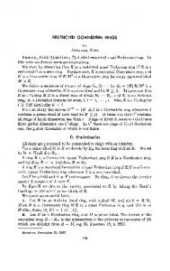
which agrees with the statement of Theorem 1.1. The value of the constant which defines the rate of decay of p2n,0 in (1.2) is 1 √ ζ (3/2) ≈ 1.0422, 2π which is consistent with its numerical estimate; see Figure 1. The numerical analysis of the exact formula for p2n,0 [see (2.2) below] also shows that under the assumption that the next-to-leading term in the large-N expansion of pN,0 is constant, the resulting coefficient (≈ 0.06267) is close to its exact counterpart from the large gap size expansion of the Derrida–Zeitak formula (≈ 0.0627). At the moment, we do not have a theory explaining this closedness. Both the numerical simulations and the heuristic argument given above provide a strong hint in favour of Theorem 1.1. There are several possible routes to the proof of the theorem. For example, one can try to use Forrester’s observation, coupled with the knowledge of the rate of convergence of the Borodin–Sinclair–Forrester–Nagao kernel in the largeN limit, to show that the errors in applying Derrida–Zeitak’s formula to gaps of N -dependent sizes vanish as N → ∞. There is however a problem with this approach: in the case we are interested in (annihilating Brownian motions or the 2-state Potts model) the infinite sums entering the gap formula converge only polynomially; see [8] for details. Therefore, a careful justification would be required for the validity of the interchange of summation and taking the large gap size limit. We feel that such a justification is best done in the context of a general theory of “Fredholm Pfaffians”. In this paper, we will adopt the spirit of Derrida–Zeitak’s

2736

E. KANZIEPER ET AL.

F IG . 1. The logarithm of the probability pN,0 that an N × N matrix of even size sampled from the √ real Ginibre ensemble does not have any real eigenvalues, as a function of N . The leading coefficient extracted using the best fit is −1.042, the best fit for the next-to-leading constant is 0.06267. The “exact” curve is constructed using formula (2.2) of Lemma 2.1 below. The form of the b2 -term in the fitting curve was chosen to minimise the numerical goodness-of-fit χ 2 .

calculation to construct rigorous asymptotics of a very compact and easy to use exact determinantal expression for the probability p2n,2k specific to the real Ginibre ensemble. This determinantal expression can be derived building upon the results of [14] and [12]; see Lemma 2.1 below. We hope of course that our very specialised proof will contribute to the general discussion of the theory of large deviations for Pfaffian point processes. There is a drawback to our approach as well: even though we can now claim that (1.2) is true, we still do not know how a large Ginibre matrix without real eigenvalues looks. For example, is there a unique optimal configuration of complex eigenvalues for such matrices? What can be said about the overlaps between left and right eigenvectors of Ginibre matrices without real eigenvalues? To answer these questions, one has to develop a large deviations principle along the lines of [7] which will most likely use the picture of the “two-component” plasma consisting of one-dimensional and two-dimensional “gases” of eigenvalues discussed there. Our paper is organised as follows: a reader who is satisfied by our heuristic argument and the numerics can stop here. Those interested in the mathematical proof are advised to read Section 2 and consult Appendix A for the proofs of the

2737

LARGE RANDOM MATRIX WITH NO REAL EIGENVALUES

technical facts used in the proof of Theorem 1.1. Appendix B contains remarks on the numerical evaluation of p2n,0 for large values of n. 2. The proof of Theorem 1.1. Our starting point is the following exact determinantal representation for the generating function for the probabilities p2n,2k . L EMMA 2.1. (2.1)

n  k=0

Let n be a positive integer. Then

z p2n,2k = det k

j,k=1,n

In particular, (2.2)



p2n,0 = det

j,k=1,n



(j + k − 3/2) (z − 1) √ δj,k + √ . (2j − 1)(2k − 1) 2π

(j + k − 3/2) 1 δj,k − √ √ . 2π (2j − 1)(2k − 1)

We postpone to Appendix A the proofs of all lemmas used during the proof of the main theorem. Notice that the expression (2.2) coincides (as it should) with the s → ∞ limit of the probability that a 2n × 2n real Ginibre matrix has no real eigenvalues in the interval (−s, s) calculated by Forrester; see formula (3.48) of [11]. We will prove Theorem 1.1 in two steps: first, we will prove (1.2) for k = 0, then we will show that limn→∞ √1 log p2n,2kn = limn→∞ √1 log p2n,0 , where 2n

2n

(kn )n≥1 is a sequence of integers which grows with n slower than n1/2 / log(n). 2.1. The calculation of limn→∞ √1 log p2n,0 . Let Mn be an n × n symmetric 2n matrix entering the statement of Lemma 2.1: (2.3)

(j + k − 3/2) 1 , Mn (j, k) = √ √ 2π (2j − 1)(2k − 1)

1 ≤ j, k ≤ n.

L EMMA 2.2. Mn is a positive definite matrix. Moreover, there exists a positive constant μ > 0 and a natural number N such that for any n > N , μ (2.4) λmax (n) ≤ 1 − , n where λmax (n) is the maximal eigenvalue of Mn . Using Lemmas 2.1 and 2.2 we represent p2n,0 as follows:

(2.5)

1 1 √ log p2n,0 = √ Tr log(I − Mn ) 2n 2n Kn 1  1 1 = −√ Tr Mnm − √ Rn (Kn ), 2n m=1 m 2n

2738

E. KANZIEPER ET AL.

where Kn is a cut-off which increases with n (chosen below) and Rn is the remainder of the Taylor series for log(I − Mn ) written in the integral form: 

 1



MnK+1 (1 − x)K dx. K+1 (1 − xM ) 0 n An upper bound on |Rn (K)| follows from Lemma 2.2 by replacing all eigenvalues of Mn with λmax (n): Rn (K) =

Tr

Rn (K) ≤ nλK+1 (n) max

 1 0

(1 − x)K dx (1 − λmax (n)x)K+1



≤ nλK max (n) log So, if we choose





Kn = nα ,

(2.6)



1 n ≤ n log 1 − λmax (n) μ



μ 1− n

K

.

α > 1,

it is easy to check that lim Rn (Kn ) = 0.

(2.7)

n→∞

The last step of the proof is the calculation of results can be summarised as follows. L EMMA 2.3.

For any fixed integer m > 0,

1 (2.8) lim √ Tr Mnm = n→∞ 2n Moreover, for any positive integers m, n 

Tr Mnm

(2.9)

≤

Kn

1 m=1 m

Tr Mnm . The relevant



1 . 2πm 

 1  1 m n  1 + n−1 + + 1 + 2n−1 . πm 4 8 πn

Let us stress that formula (2.8) alone is not enough for the calculation of the limn→∞ n−1/2 log p2n,0 using (2.5) since the limits n → ∞ and m → ∞ do not necessarily commute. Instead, let us fix an arbitrary integer K > 0. For a sufficiently large n (so that Kn > K), relation (2.9) gives K 1 1  √ Tr Mnm 2n m=1 m

(2.10)

Kn 1 1  Tr Mnm ≤√ 2n m=1 m

≤

Kn Kn Kn 1  (1 + n−1 )  (1 + 2n−1 )  1 1 √ √ . m−3/2 + √ + √ 2π m=1 4 2n k=1 m 8 2π n k=1 m

LARGE RANDOM MATRIX WITH NO REAL EIGENVALUES

2739

In writing the above double inequality, we used the fact that Mn is positive definite, which implies that Tr Mnm > 0 for all values of m, n. Let us choose Kn in the form (2.6) with α < 2 and take n → ∞ in (2.10). As K is n-independent, we can use formula (2.8) to compute the limit of the left-hand side. On the right-hand side, the √ last two sums vanish in the limit [as log(n)/ n and nα/2−1 correspondingly]. The first sum converges to



∞ 1  1 √ m−3/2 = √ ζ (3/2), 2π m=1 2π

−x is the Riemann zeta-function. where ζ (x) = ∞ m=1 m We have found that for any positive integer K, Kn K 1  1 1  √ Tr Mnm m−3/2 ≤ lim inf √ n→∞ m 2π m=1 2n m=1 Kn 1  1 Tr Mnm ≤ lim sup √ m n→∞ 2n m=1

1 ≤ √ ζ (3/2). 2π As K is arbitrary, we conclude that (2.11)

Kn 1  1 Tr Mnm = √ ζ (3/2). lim √ n→∞ 2n 2π m=1

So we proved that both (2.7) and (2.11) hold provided the cut-off is taken in the form (2.6) for any fixed α ∈ (1, 2). Finally, we can take the n → ∞ limit in (2.5). Employing (2.7) and (2.11), we find that 1 1 lim √ log p2n,0 = − √ ζ (3/2). n→∞ 2n 2π Theorem 1.1 is proved for k = 0. 2.2. The calculation of limn→∞ √1 log p2n,2k for k > 0. It follows from 2n Lemma 2.1 that 

p2n,2k =

1 d k! dz

k





det I + (z − 1)Mn

z=0

Equivalently, 

(2.12)

p2n,2k =

p2n,0 d k! dz

k



det(I + zPn )

z=0

,

.

2740

E. KANZIEPER ET AL.

where Pn = (I − Mn )−1 Mn . Recall that det(I + zPn ) =

n 

zk ek (ν),

k=0

where ν = (ν1 , ν2 , . . . , νn ) are the eigenvalues of Pn and ek is the degree-k elementary symmetric polynomial in n variables [15], ek (ν) =



νi1 νi2 · · · νik .

1≤i1 0 there is a positive integer Nε such that for any n > Nε 

(2.16)

n (1 − ε) ≤ Tr Mn ≤ π



n (1 + ε). π

On the other hand, (2.17)

Tr Mn = (λ1 + · · · + λk−1 ) + (λk + · · · + λn ) ≤ (k − 1) + (n − k + 1)λk ,

where the inequality is due to (2.4) and the chosen ordering of λ’s. Combining (2.16) and (2.17), we obtain the following bound on the kth largest eigenvalue of Mn : √ n/π (1 − ε) − k + 1 (2.18) , λk ≥ n−k+1

LARGE RANDOM MATRIX WITH NO REAL EIGENVALUES

2741

which holds for n > Nε . Inequality (2.18) leads to the desired bound for ek (ν): √  n/π (1 − ε) − k + 1 k k . ek (ν) ≥ ek (λ) ≥ λ1 λ2 · · · λk ≥ λk ≥ n−k+1 Substituting this result into (2.13), we find that √  n/π (1 − ε) − k + 1 log p2n,2k ≥ log p2n,0 + k log (2.19) . n−k+1 Combining (2.15) and (2.19), we find that 1 1 lim √ log p2n,2k = lim √ log p2n,0 . n→∞ 2n 2n Relations (2.20) and (2.1) imply that formula (1.2) of Theorem 1.1 is proved for any fixed integer k > 0. Moreover, it is evident from (2.15) and (2.19) that equality (2.20) generalises to (2.20)

(2.21) where (kn )n≥1

n→∞

1 1 lim √ log p2n,2kn = lim √ log p2n,0 , n→∞ 2n n→∞ 2n is a sequence of natural numbers such that 



lim n−1/2 log(n) kn = 0.

n→∞

This proves the last claim of Theorem 1.1. R EMARK . Our proof of the k > 0 part of the theorem is a simple consequence n→∞ of √ positive-definiteness of Mn , the spectral bound and the fact that Tr(Mn ) ∼ n/π . It is interesting that the proof does not rely on any detailed knowledge of the spectrum of Mn . APPENDIX A: PROOFS FOR THE LEMMAS A.1. Proof of Lemma 2.1. To prove the lemma, we start with the exact formula due to Kanzieper and Akemann [14] which expresses the probabilities p2n,2k in terms of elementary symmetric functions: (A.1)

p2n,2k = p2n,2n en−k (t1 , . . . , tn−k ),

where tj ’s are given by (A.2)



j

tj = 12 Tr A−1 B .

Here, A and B are 2n × 2n antisymmetric matrices whose entries (A.3)

Aj k = qj −1 , qk−1 R ,

(A.4)

Bj k = qj −1 , qk−1 C ,

2742

E. KANZIEPER ET AL.

are defined in terms of skew products  1 2 2 (A.5) dx dye−(x +y )/2 sgn(y − x)f (x)g(y)

f, gR = 2 2 R and     z − z¯  2 −(z2 +¯z2 )/2 (A.6) f, gC = i d ze erfc √ f (z)g(¯z) − g(z)f (¯z) . Imz>0 i 2 Let us stress that (A.1) is valid for an arbitrary choice of monic polynomials qj (x) of degree j , provided matrix A is invertible. Substituting equations (A.1) and (A.2) into the generating function g2n (z) =

(A.7)

n 

zk p2n,2k

k=0

and making use of the summation formula [15] (A.8)

∞ 

z e (t1 , . . . , t ) = exp 

∞ 



(−1)

j −1

j =1

=0

zj tj , j

we obtain the Pfaffian representation [2, 5, 14]: (A.9)





g2n (z) = p2n,2n Pf −A−1 Pf(zA + B);

see remark 1.3 of [5] justifying the transition from square roots of determinants to Pfaffians. Since g2n (1) = 1, p2n,2n = (Pf(−A−1 ) Pf(zA + B))−1 and (A.9) simplifies to Pf(zA + B) (A.10) . g2n (z) = Pf(A + B) Next, we will use the fact that expression (A.10) for the generating function does not depend on a particular choice of monic polynomials qj (x) in (A.3) and (A.4) to simplify it even further. Namely, we will choose qj (x)’s in such a way that the matrix A + B is block diagonal. Clearly, such polynomials should be skeworthogonal with respect to the skew product (A.11)

f, g = f, gR + f, gC ,

that is (A.12)

q2j , q2k+1  = − q2k+1 , q2j  = rj δj,k ,

q2j , q2k  = q2j +1 , q2k+1  = 0.

These were first calculated in the paper [12]: (A.13)

q2j (x) = x 2j , q2j +1 (x) = x 2j +1 − 2j x 2j −1 , √ rj = 2π (2j + 1).

Given the choice of qj ’s described above:

2743

LARGE RANDOM MATRIX WITH NO REAL EIGENVALUES

(a) the matrix A + B acquires a block-diagonal form, A + B = r ⊗ J, where 

r = diag(r0 , . . . , rn−1 ),

(A.14)

J=



0 1 , −1 0

which leads to g2n (z) =

(A.15)

Pf(r ⊗ J + (z − 1)A) . Pf(r ⊗ J)

(b) the matrix A is given by (A.16)



A2j,2k = A2j +1,2k+1 = 0,

A2j −1,2k =  j + k −

3 2 .

Notice that matrix elements of both r ⊗ J and A labeled by a pair of indexes of the same parity vanish. Therefore, the 2n × 2n Pfaffians in the numerator and the denominator of (A.15) are reduced to n × n determinants: (A.17)

g2n (z) =

det[rj −1 δj k + (z − 1)A2j −1,2k ]1≤j,k≤n . det[rj −1 δj k ]1≤j,k≤n

Finally, we apply the formula det(U )/ det(V 2 ) = det(V −1 U V −1 ) to perform division in (A.17). With the help of the explicit formulae (A.13) and (A.16) we get

(A.18)

(j + k − 3/2) (z − 1) √ g2n (z) = det δj k + √ (2j − 1)(2k − 1) 2π



. 1≤j,k≤n

Lemma 2.1 is proved. A.2. Proof of Lemma 2.2. The proofs of Lemmas 2.2, 2.3 are based on the following integral representation for the matrix elements (2.3) of matrix Mn : (A.19)

1 Mn (j, k) = √ 2π

 ∞ dx

xk xj −x √ √ e , x 5/2 (2j − 1) (2k − 1)

0

1 ≤ j, k ≤ n, which can be obtained by representing (j + k − 3/2) in (2.3) as an integral. Take any v = (v1 , v2 , . . . , vn ) ∈ Rn \ {0}. It follows from (A.19) that (A.20)

1

v, Mn v = √ 2π

 ∞ dx

x 5/2

0

e

−x

 n 

vj x j √ (2j − 1) j =1

2

> 0.

So, Mn is positive definite by definition. Next, let us prove bound (2.4) on the spectral radius of Mn . Let λ1 , λ2 , . . . , λn > 0 be the eigenvalues of Mn . Then (A.21)

λmax

 (n) = λn

1/n

max (n)

≤

 n  k=1

1/n

λnk



= Tr Mnn

1/n

.

2744

E. KANZIEPER ET AL.

It follows from the upper bound (2.9) of Lemma 2.3 that for any ε > 0, there is Nε such that for any n > Nε , 



1 1 1 1 + + + ε = 1 − c1 + ε, Tr Mnn ≤ π 4 8 π where c1 ∈ (0, 1). Therefore, we can choose ε small enough so that Tr Mnn ≤ 1 − μ, where μ ∈ (0, 1). Using this estimate in (A.21) for n > Nε we get μ (A.22) λmax (n) ≤ (1 − μ)1/n ≤ 1 − . n Lemma 2.2 is proved for N = Nε . R EMARK . The spectral properties of Mn seem quite interesting. For instance, in the large-n limit there is a concentration of eigenvalues near 1 such that the restriction of Mn to the space spanned by the corresponding eigenvectors is close to an identity operator perturbed by an elliptic linear differential operator. Formal analysis of this perturbation suggests the asymptotic λmax (n) = 1 − μ0 n−1 + o(n−1 ) for suitable μ0 > 0. A.3. Proof of Lemma 2.3. The integral representation (A.19) for the matrix elements of Mn leads to the following integral representation for the trace of a power of Mn :  ∞  ∞  ∞ dx1 dx2 dxm −x1 −x2 −···−xm √ √ √ Tr Mnm = ··· e 2πxm 2πx1 0 2πx2 0 0 (A.23) √ √ √ × coshn−1 ( xm x1 ) coshn−1 ( x1 x2 ) · · · coshn−1 ( xm−1 xm ), 

2k

x where coshn (x) = nk=0 (2k)! is the degree-2n Taylor polynomial generated by the hyperbolic cosine. Performing the change of variables xk = yk2 in (A.23), we can rewrite the integral representation for Tr Mnm as follows:



Tr Mnm = (A.24)

2 π

m/2 

Rm +

dye−

m

2 k=1 yk

× coshn−1 (ym y1 ) coshn−1 (y1 y2 ) · · · coshn−1 (ym−1 ym ).

m Here, Rm + = {(y1 , y2 , . . . , ym ) ∈ R |yk ≥ 0, k = 1, 2, . . . , m} is the first “quadm rant” of R and dy is a shorthand notation for Lebesgue measure on Rm . As the integrand of (A.24) is symmetric with respect to reflection yi → −yi for any i = 1, 2, . . . , m, we can rewrite Tr Mnm as an integral over Rm :



Tr Mnm (A.25)

1 = 2π

m/2 

Rm

dye−

m

2 k=1 yk

× coshn−1 (ym y1 ) coshn−1 (y1 y2 ) · · · coshn−1 (ym−1 ym ).

2745

LARGE RANDOM MATRIX WITH NO REAL EIGENVALUES

To prove Lemma 2.3, we will establish an upper and a lower bound on Tr Mnm and then compute the large-n limit of each of these bounds. A.3.1. An upper bound for Tr Mnm . A good starting point for the calculation is formula (A.25). For any x ∈ R, coshn−1 (x) ≤ cosh(x). Also, coshn−1 (x) =

(A.26)



dz 1 − z−2n zx e , 2πiz 1 − z−2

where the integral is anti-clockwise around a circle of radius smaller than 1 centred at the origin in the complex plane. Replacing all but one coshn−1 with cosh we get: Tr Mnm ≤ (A.27)







m/2



m 1 m/2 2 dye− k=1 yk coshn−1 (ym y1 ) cosh(y1 y2 ) · · · 2π Rm × cosh(ym−1 ym )

1 = 2π

Eα1 α2 ···αm−1

× coshn−1 (ym y1 )e

 Rm

m−1 l=1

m

dye−

αl yl yl+1

2 k=1 yk

,

where α1 , α2 , . . . , αm−1 are independent identically distributed random variables which take values ±1 with probability 1/2. Representing the remaining coshn−1 with the help of (A.26) and then computing resulting Gaussian integral over Rm , we find (A.28) where

Tr Mnm

≤

 m/2 1

⎛

1 ⎜ ⎜ α1 ⎜− ⎜ 2 ⎜ ⎜ ⎜ 0 ⎜ ⎜ ⎜ · ⎜ (α) Dm (z) = det ⎜ ⎜ · ⎜ ⎜ · ⎜ ⎜ 0 ⎜ ⎜ ⎜ ⎜ 0 ⎜ ⎝

−

(A.29)

z 2

2

Eα1 α2 ···αm−1

α1 2 1 α2 − 2 · · · ...

0 α2 − 2 1 · · · 0

... 0

−



dz 1 − z−2n  (α) −1/2 Dm (z) , 2πiz 1 − z−2 0

...

0

0

...

0

0 α3 − 2 · · · αm−3 − 2 0

...

0

0 · · · 1 αm−2 − 2 0

... · · · αm−2 − 2 1 αm−1 − 2

z 2 0

−

⎞

⎟ ⎟ ⎟ ⎟ ⎟ ⎟ 0 ⎟ ⎟ ⎟ · ⎟ ⎟ ⎟. · ⎟ ⎟ · ⎟ ⎟ 0 ⎟ ⎟ ⎟ αm−1 ⎟ ⎟ − 2 ⎟ ⎠

1

2746

E. KANZIEPER ET AL. (α)

The determinant can be calculated recursively in m, yielding D1 (z) = 1 − z and 

(A.30)

(α) Dm (z) = −(m − 1)



m+1 1 (z − A ) z + A m m 2m m−1



for m ≥ 2,

where Am = m−1 k=1 αk . Note that (A.30) implies that all principal minors of the matrix under the sign of the determinant in (A.29) are positive for z = 0. Therefore, the matrix itself is positive definite for z = 0. By continuity, the real part of this matrix remains positive definite for z = 0 provided |z| is small enough. Therefore, the real part of the quadratic form which determines the Gaussian integral in (A.27) is positive definite, which justifies the interchange of integrals leading to (A.28) provided the contour is taken to be a circle around the origin of a sufficiently small radius. Substituting (A.30) into (A.28) and changing the integration variable z → Am z, we find that the integrand no longer depends on α’s. Averaging over α’s becomes trivial and we get the following integral upper bound: (A.31)

Tr Mnm

≤



1 dz z−2n − 1 1 √ √ . 2πz z−2 − 1 1 − z (m − 1)z + m + 1

The rest of the calculation is slightly different depending on whether m = 1 or m > 1. Here, present the calculation for m > 1 only, the (simpler) case of m = 1 can be treated along similar lines. We calculate the integral in the right-hand side of (A.31) as follows. First, we replace z−2n − 1 with z−2n in the integrand on the right-hand side of (A.31), since this does not change the value of the integral as the omitted term is analytic inside of the contour of integration. Next, we deform the contour away from the singularity at zero and out to infinity, leading to integrals around the other singularities of the (modified) integrand: a simple pole at z = −1, a branch cut singularity along the real line from 1 to +∞, and a branch cut singularity along the real line from − m+1 m−1 to −∞. The contribution from the integral over the large circle at infinity is zero. The contribution from the pole at z = −1 is easily evaluated as 1/4. Evaluating the integral around the branch from 1 to +∞ it is convenient first integrate by parts, so that the singularity at z = 1 is integrable. The integrals along the two branch cuts lead to two real integrals whose asymptotics are controlled by the integrand (1 + y)−2n . Changing variable y → y/2n, and making some simple estimates on terms that do not affect the leading asymptotics, we are led to Tr Mnm (A.32)

1 ≤ + 4



n πm

  ∞ dy 0

y 1+ √ πy 2n 

m+1 m+1 √ +√ 2πn 2 m − 1 2m 1

×

  ∞ dy 0

y 1+ √ πy 2n

−2n

3/2 

−2n+1

.

m−1 m+1

2n+1

2747

LARGE RANDOM MATRIX WITH NO REAL EIGENVALUES

Both integrals in the above expression can be estimated using the following bound: IM =

(A.33)

  ∞ dy

√ πy

0

y M

1+

−M

≤1+

2 , M

which follows by evaluating the integral, using the substitution t = (1 + terms of the beta function as 

IM =



y −1 M) ,

in



√ (M − 3/2) M 1 1 B M− , = M π 2 2 (M − 1/2)

and using bounds on the Gamma function. Using this in (A.32), the final result is Tr Mnm (A.34)

1 ≤ + 4

 





















n 1 1 m 2 1+ + 1+ πm n 8 πn n

m−1 m+1

2n−3/2

n 1 1 1 m 2 ≤ + 1+ + 1+ , 4 πm n 8 πn n which coincides with the claim (2.9)√of Lemma 2.3. Dividing both sides of (A.34) by 2n and taking the large n limit, we find that 

1 lim sup √ Tr Mnm ≤ n→∞ 2n

(A.35)

1 . 2πm

A.3.2. The limit limn→∞ √1 Tr Mnm . The strategy is to derive an integral 2n lower bound for Tr Mnm and calculate the large n-limit of the bound. Our starting point is the relation (A.24) and the following estimate for the polynomial coshn−1. L EMMA A.1.

(A.36)

There exist two sequences (hn )n≥1 , (Sn )n≥1 ⊂ R such that 1 lim hn = , n→∞ 2

lim Sn = 2,

n→∞

e−ny coshn−1 (ny) ≥ hn 1(y < Sn )

for y ≥ 0, n ≥ 1.

Here, 1(y < Sn ) is the indicator function of the set [0, Sn ). In fact, as n → ∞, e−ny coshn−1 (ny) converges almost everywhere to 12 1(y < 2) for y ≥ 0, but here we only need the lower bound. The proof of Lemma A.1 is given in Section A.4. Using the bound (A.36) in (A.24), we find that 

Tr Mnm

≥ hm n

(A.37) ×

2 π

m  l=1

m/2

nm/2

 Rm +

dy

1(yl yl+1 < Sn )e−(n/2)

m

k=1 (yk+1 −yk )

2

,

2748

E. KANZIEPER ET AL.

where ym+1 := y1 . It is straightforward to verify that √ the domain of integration for the integral in (A.37) contains the hypercube (0, Sn )m , 





m (0, Sn )m ⊂ y ∈ R+ |yk yk+1 < Sn , k = 1, 2, . . . , m .

Therefore, (A.38)

n 

m 



1(yl < Sn ) ≤

l=1

y ∈ Rm +

1(yl yl+1 < Sn ),

l=1

Substituting (A.38) in (A.37) and changing the integration variables according to R = y1 + y2 + · · · + ym , zk = yk+1 − yk ,

k = 1, 2, . . . , m − 1,

we get the following lower bound: 

Tr Mnm (A.39)

hm 2 ≥ n m π ×

m/2

n

m/2

 m√Sn

dR 0



m−1 2 m−1 2 k=1 zk +( k=1 zk ) ]

Pm−1 (R)

dz1 · · · dzm−1 e−(n/2)[

,

√ where Pm−1 (R) is the intersection of the hypercube (0, Sn )m and the hyperplane 



m y ∈ R+ |y1 + y2 + · · · + ym = R .

In the derivation of (A.39), we used the fact that the Jacobian of the transformation y → (R, z) is equal to 1/m. The large-n limit of the right-hand side of (A.39) can be evaluated by arguing as in the Laplace method: 1 lim inf √ Tr Mnm n→∞ 2n



hm 2 ≥ lim √ n n→∞ 2nm π ×



Rm−1

n→∞

 Rm



n→∞

 m√Sn

dR 0

dz1 · · · dzm−1 e−(n/2)[ 

Sn m 2 h 2 n π

= lim

= lim

n

m/2

m−1 2 m−1 2 k=1 zk +( k=1 zk ) ]



×

m/2

m/2

dz1 · · · dzm eiλ 

Sn m 2 h 2 n π

n(m−1)/2 m

k=1 zk

m/2

n

 ∞ dλ −∞

e−(n/2)

(m−1)/2

2π m

2 k=1 zk

 ∞  ∞ dλ −∞

2π

−∞

dze

iλz−(n/2)z2

m

LARGE RANDOM MATRIX WITH NO REAL EIGENVALUES



= lim

n→∞



= lim

n→∞



Sn m 2 h 2 n π 

Sn m 2 h 2 n π

m/2



n(m−1)/2

m/2



n

(m−1)/2

2749

m/2  ∞ dλ −(m/(2n))λ2 e

2π n

−∞

m/2 

2π n

2π

n = 2πm



1 . 2πm

The crucial, albeit very standard, first step in the above derivation consists of verifying that extending the integration space for the z-integral from Pm−1 (R), when R ∈ (0, 2), to Rm−1 does not change the large n-limit. We conclude that 

1 lim inf √ Tr Mnm ≥ n→∞ 2n

1 , 2πm

and in combination with (A.35) this gives 

1 lim √ Tr Mnm = n→∞ 2n

1 . 2πm

Statement (2.8) of Lemma 2.3 is proved. A.4. Proof of Lemma A.1. Let {αn }∞ n=1 be an arbitrary sequence of positive real numbers which diverges as n → ∞ slower than n1/2 , that is limn→∞ αn = ∞, but limn→∞ αn n−1/2 = 0. We will show that there exists N0 > 0 such that for any n > N0 and x ≥ 0 (A.40)

e

−nx





  1 1 2 coshn (nx) ≥ − √ αn−1 e−αn /4 1 x ≤ 2 − αn n−1/2 . 2 4π

The statement of Lemma A.1, where coshn (nx) is replaced by coshn−1 (nx), is easily deduced from equation (A.40). Our proof builds on the ideas of [4] dedicated to the study of sections of exponential series (Taylor polynomials generated by exp). Let en be a section of exponential series defined by en (x) =

n  xj j =0

j!

.

Consider also en(+) (x) = e−nx en (nx),

en(−) (x) = e−nx en (−nx).

Then the function we are interested in can be written as fn (x) := e−nx coshn (nx) =



 

 

1 (+) x (−) x e2n + e2n 2 2 2

.

2750

E. KANZIEPER ET AL. (−)

First, we show that e2n (x) > 0 for x ≥ 0. One can check that (A.41)

 d  2nx 1 (2nx)2n e2nx ≥ 0, e e2n (−2nx) = dx (2n − 1)!

and e2nx e2n (−2nx)|x=0 = 1. So e2n (x) ≥ e−4nx > 0 for x ≥ 0. The next step is to show that fn (x) is a decreasing function. However, (−)

(−) fn (x) = −ne2n

 

x , 2

which is negative by (A.41). (−) The fact that fn (x) is decreasing and the positivity of e2n (x) imply that for any nonnegative x 

fn (x) ≥ fn (x)1 x ≤ 2 − αn n−1/2 



 

≥ fn 2 − αn n−1/2 1 x ≤ 2 − αn n−1/2 





  1 (+) αn ≥ e2n 1 − n−1/2 1 x ≤ 2 − αn n−1/2 . 2 2

Therefore, it remains to prove that (A.42)

(+) e2n







αn 1 − n−1/2 ≥ 1 − 2

1 −1 −αn2 /4 α e , π n

for all n > N0 , where N0 is chosen to satisfy αn n−1/2 < 2 for all n > N0 . We start with a differential equation satisfied by en(+) . As it is easy to check, (A.43)

1 d (+) en (x) = − (nx)n e−nx . dx (n − 1)!

So en(+) (x) is a decreasing function on R+ . Equation (A.43) has to be solved with a boundary condition limx→∞ en(+) (x) = (+) 0, which follows from the definition of en . The solution is (A.44) Let

en(+) (x) =

nn (n − 1)!

 ∞

t n e−nt dt.

x

√ 2πn(n/e)n φn = . n!

By the Stirling approximation formula, φn = 1 + O(n−1 ) for n → ∞ and φn < 1. Define (A.45)

τ (t) = t − 1 − log t ≥ 0

for t ∈ R+ .

LARGE RANDOM MATRIX WITH NO REAL EIGENVALUES

2751

In terms of φn and τ , expression (A.44) acquires the following form: 



∞ n φn (A.46) e−nτ (t) dt. 2π x The integral in the right-hand side can be analysed using the Laplace method. It follows from the definition that   ∞ n 1 = en(+) (0) = e−nτ (t) dt. φn 2π 0 Therefore, (A.46) can be rewritten as follows:   x n (+) en (x) = 1 − e−nτ (t) dt =: 1 − rn (x). φn 2π 0 Let us estimate the remainder rn (x). Evidently, rn (x) ≥ 0. An application of Taylor’s theorem with the Lagrange form of the remainder reveals that for 0 < t ≤ x ≤ 1,

en(+) (x) =

τ (t) ≥

(A.47)

τ  (x) (t − x)2 + τ  (x)(t − x) + τ (x). 2

1  Noticing that τ  (x) = − 1−x x and τ (x) = x 2 we can use the above bound on τ (t) to obtain the following upper bound on rn :



rn (x) ≤

n φn e−nτ (x) 2π

 x

e−(n/(2x

0

2 ))(t−x)2 +(n(1−x)/x)(t−x)







dt





n n φn −n(τ (x)−(1−x)2 /2) erfc xe (1 − x) − erfc (2 − x) 2 2 2   n φn (1 − x) , ≤ xe−nτ (x) erfcx 2 2 where erfc and erfcx are complementary and scaled complementary error functions correspondingly. Finally, applying the classical estimate erfcx(x) ≤ x √1 π valid for any x > 0 (see, e.g., [1]), we obtain x −nτ (x) x −nτ (x) φn 1 rn (x) ≤ √ e e