Perception & Psychophysic s 2002, 64 (4), 570-583
What makes a categorization task difficult? LEOLA A. ALFONSO-REESE San Diego State University, San Diego, California and University of California, Santa Barbara, California and F. GREGORY ASHBY and DAVID H. BRAINARD University of California, Santa Barbara, California To understand why some categorization tasks are more difficult than others, we consider five factors that may affect human performance—namely, covariance complexity, optimal accuracy level with and without internal noise, orientation of the optimal categorization rule, and class separability. We argue that covariance complexity, an information-theoretic measure of complexity, is an excellent predictor of task difficulty. We present an experiment that consists of five conditions using a simulated medical decision-making task. In the task human observers view hundreds of hypothetical patient profiles and classify each profile into Disease Category A or B. Each profile is a continuous-valued, three-dimensional stimulus consisting of three vertical bars, where each bar height represents the result of a medical test. Across the five conditions, covariance complexity was systematically manipulated. Results indicate that variation in performance is largely a function of covariance complexity and partly a function of internal noise. The remaining three factors do not explain performance results. We present a challenge to categorization theorists to design models that account for human performance as predicted by covariance complexity.
Some categorization tasks are easier to perform than others. For example, it is easier to classify Siamese versus Sphinx cats than Siamese versus Himalayans. Many factors affect the difficulty of such tasks—for example, stimulus dimensionality, number of relevant dimensions, correlations between dimensions, and category overlap. Each of these factors is determined by category structure. In this study, we systematically manipulated category structure and characterized its effect on human performance using accuracy and efficiency measures. In particular, we try to show that a specific aspect of category structure, covariance complexity, is an excellent predictor of task difficulty. Covariance complexity is an information-based characterization of the covariance matrix that shapes our categories. This measure is formally defined below. The relationship between category structure and task difficulty has been of interest to psychologists for several decades. It was examined by Shepard, Hovland, and Jenkins (1961) in their classic study, Learning and memorization of classifications. They found that the order of difficulty, measured in number of errors, could be predicted by the number of dimensions required to specify the categories. Furthermore, they suggested that when the number of relThanks to Robin Thomas and two anonymous reviewers for their helpful comments on an earlier draft of this paper. Thanks also to Elliot Waldron for running Condition 5. Correspondence should be addressed to L. A. Alfonso-Reese, San Diego State University, Department of Psychology, 5500 Campanile Drive, San Diego, CA 92182-4611 (e-mail:
[email protected]).
Copyright 2002 Psychonomic Society, Inc.
evant dimensions, say d, is equal in two different tasks, one task might be easier than another if a portion of the stimuli in that task can be correctly classified using fewer than d dimensions. Bourne (1970) also ordered the difficulty of categorization tasks in his famous study on rule learning. He found that conjunctive rules are easier than disjunctive, followed by conditional, then biconditional rules. The present study extends this previous work by proposing a formal measure for predicting categorization difficulty and by using artificial categories that embody qualities of natural categories—for example, the categories overlap and the stimuli differ along continuous-valued dimensions. A second goal of our study was to extend previous categorization research from use of bivariate continuous dimensions (e.g., Ashby & Gott, 1988; Ashby & Maddox, 1990; McKinley & Nosofsky, 1995) to use of trivariate continuous dimensions. This extension is important because individual exemplars of natural categories often differ along many continuous-valued dimensions (e.g., Ashby, 1992). For example, trees vary continuously in height, girth, hue, and texture. Yet, few categorization studies have used stimuli that vary parametrically along more than two continuous dimensions (e.g., Homa, Sterling, & Trepel, 1981; Posner & Keele, 1968, 1970). First, we introduce the trivariate categorization task and the experimental design. We specify category structure and discuss factors that affect task difficulty. This discussion includes predictions for performance across five conditions based on our manipulation of category structure. Then, we present an experiment involving more than
570
CATEGORIZATION DIFFICULTY 1,500 trials of data from each of 30 participants who participated in one of the five conditions. Finally, we summarize our results and discuss possible future directions for this line of research. Our Trivariate Categorization Task The experimental paradigm employed is the general recognition randomization technique. This technique was developed to investigate decision processes, and it has been successfully applied to one- and two-dimensional categorization data (e.g., Ashby & Maddox, 1992; Maddox & Ashby, 1993; McKinley & Nosofsky, 1995). Given that the paradigm has been fully described in several previous publications (e.g., Ashby, 1992; Ashby & Gott, 1988; Ashby & Maddox, 1992), we do not reintroduce it here; rather, we present necessary details pertaining to our particular categorization task. An example of the stimulus used on each trial is shown in Figure 1. Each stimulus was a hypothetical patient’s profile consisting of three bars where each bar height represented the outcome of a medical test. The bars were labeled “BP” for blood pressure level, “WBCs” for white blood cells, and “serK” for serum potassium level. For each participant, the height of the three bars differed across trials, while the labels remained the same. Participants were told that the purpose of the experiment was to study the process physicians use when diagnosing diseases. Also, participants were instructed to act as a physician and decide whether each of many patients had Disease A or Disease B. Feedback about accuracy was provided after each response, but participants had no training before giving their first response. In each condition, participants classified hundreds of these three-dimensional stimuli, one at a time, into one of the two categories, A or B. Each category was specified by a trivariate normal distribution, and the heights of the three bars that defined each stimulus were specified by a point randomly sampled from one of these distributions. The point coordinates of each stimulus were converted to a threebar pattern, where each coordinate value determined the height of one bar. For example, the B prototype stimulus for Participant 1 in Condition 1 was a three-bar stimulus generated from the coordinate vector [207 207 148]¢, where the prime denotes “transpose” (Figure 1). Trivariate normal distributions were specified by nine parameters: a mean and variance on each of the three stimulus dimensions and a covariance between each pair of dimensions. For notational convenience, we refer to the three dimensions as b, w, and k. The distribution parameters are typically collected as a mean vector m and covariance matrix S , defined as é s2 é mb cov bw cov bk ê b ê m = êmw , å = êcov bw cov wk , s w2 ê ê mk s k2 ë êë cov bk cov wk where, for example, mb and s b2 are the trial-by-trial mean and variance, respectively, of the height of the bar labeled
571
“BP,” and covbw is the trial-by-trial covariance between the heights of the bars labeled “BP” and “WBCs.” Note that the prototype of each category is completely specified by its mean vector. In all of our conditions, the means of the A and B category distributions differed, m A Þ m B, and the covariance matrices were identical, SA = SB . The optimal strategy for classifying stimuli drawn from normal distributions with equal variance–covariance matrices is to use a linear decision bound (e.g., Ashby, 1992; Duda & Hart, 1973). We restricted the optimal decision bounds to the linear class so that (1) the form of the optimal boundary would be constant across conditions, and (2) we could compare results of the present study with those of previous work involving linear decision bounds. The categorization problem for Condition 1 is illustrated in Figure 2. The figure shows two spheres separated by a plane. Each sphere represents an equal likelihood contour for a trivariate normal distribution. Another equivalent interpretation is that each point on a sphere is the same number of standard deviation units from the category mean (i.e., prototype). In general, the equal likelihood contours for trivariate normal distributions are ellipsoids. They are spheres in the special case where the variances on all three dimensions are equal and the pairwise covariances are all zero. To maximize percent correct, the participant should employ the deterministic strategy of classifying all stimuli that fall on the left side of the plane as A and all on the right as B. Thus the plane forms a decision bound that partitions the stimulus space into two category regions. Category Structure Throughout this study categories were defined by trivariate normal distributions. Thus, category structure was
BP
WBCs
serK
Figure 1. Example of a stimulus that was presented to participants in each condition. Each stimulus was a hypothetical patient’s profile, consisting of three bars where each bar height represented the outcome of a medical test. The bars were labeled “BP” for blood pressure level, “WBCs” for white blood cells, and “serK” for serum potassium level. The participant’s task was to indicate whether the hypothetical patient had Disease A or Disease B. The coordinates for this stimulus are 207, 207, and 148, corresponding to the height of the bars from left to right.
572
ALFONSO-REESE, ASHBY, AND BRAINARD
A
optimal decision bound
200
k
B
150
250
100 150
200 200 250
b
150
w
Figure 2. Equal likelihood contours of trivariate normal distributions from Condition 1 separated by a discriminating plane. Although the distributions extend infinitely outward, most of the samples are located within the central areas of each distribution.
completely determined by 12 parameters associated with these distributions: two category distribution means (3 parameters each) and one common covariance matrix (6 parameters). Table 1 provides the parameter values that define the A and B categories for each condition. Because correlations are easier to interpret than covariances, corresponding correlation values, ri, are also reported. In Conditions 1 and 5, the variances were equal across dimensions and all correlations were zero. In Condition 2, the variances were again equal, and all the correlations were nonzero but equal in magnitude. In Condition 3, no two variances were equal, and two correlations were approximately equal in magnitude. In Condition 4, no two variances or correlations were equal. The stimuli generated by random draw from the distributions specified in Table 1 are presented in Figure 3. Plus symbols represent stimulus vectors randomly picked from the Category A distribution, and circles represent vectors randomly picked from the Category B distribution. Each solid line is the edge of a plane representing the optimal decision boundary. Next we briefly consider several factors that may affect task difficulty and derive their predictions—namely, the order of conditions from least to most difficult.
problem) is easier than learning to classify lines that vary in length and orientation (a two-dimensional problem), assuming that length and orientation are uncorrelated. Thus, high-dimensional categorization problems tend to be more difficult than low-dimensional problems. In this study we were interested in factors that have less obvious consequences; therefore, factors like a change in dimensionality were invariant across our conditions. Other factors are discussed below. Covariance complexity. Complexity may be defined in several ways. We adopt van Emden’s (1971, p. 7) definition of complexity, “the way in which a whole is different from the composition of its parts.” Applied to a covariance matrix, complexity is a measure of the interactions of the random variables associated with the covariance matrix. Van Emden considered the multivariate normally distributed random vector for which S is the covariance matrix and derived an initial mathematical definition of covariance complexity. He noted that this definition was problematic, however, because it depends on the coordinates of the original random variables. Following van Emden, Bozdogan (1990) derived a definition of covariance complexity that is not coordinate dependent:
Factors That May Affect Categorization Difficulty Some factors affect categorization difficulty in obvious ways. For example, consider stimulus dimensionality. Learning to classify lines that vary in length (a one-dimensional
Covariance complexity = C ( å ) rank ( å ) é trace( å ) = ln ê - 1 ln det( å ) , 2 2 ë rank ( å ) where rank(S ) is the number of linearly independent rows or columns of the S matrix, the trace of a matrix is the sum
[
]
CATEGORIZATION DIFFICULTY
573
Table 1 Distribution Specifications for the Stimuli Used in Conditions 1–5 Trivariate Normal Distribution Characteristics Condition
Category A Mean
1
m
2
A
m
3
A
m
4
m
5
m
A
é177 ê = ê177 ê177 ë
Category B Mean
m
é171 ê = ê171 ê171 ë
m
é170 ê = ê170 ê170 ë
m
B
B
A
é162 ê = ê181 ê153 ë
m
A
é187 ê = ê187 ê168 ë
m
B
é207 ê = ê207 ê148 ë é188 ê = ê153 ê153 ë é190 ê = ê150 ê161 ë
B
é186 ê = ê168 ê141 ë
B
é197 ê = ê197 ê157 ë
of the elements on the main diagonal, and det (S) is the determinant of S . In all our applications, rank (S) = 3. C(S) is an upper bound to van Emden’s term. As such, it “measures both inequality among the variances and the contribution of the covariances in S” (Bozdogan, 1990, p. 241). Specifically, C( S) increases with inequality among the variances in S and with the existence of nonzero covariances. We hypothesize that as covariance complexity increases, task difficulty increases. Covariance complexity values for Conditions 1 through 5 are 0, 0.7, 1.8, 1.8, and 0. Note that the complexities for Conditions 3 and 4 are equal because the covariance matrix for Condition 4 was generated by merely changing the coordinate system for the covariance matrix in Condition 3. Complexity indicates that Conditions 1 and 5 should be easiest (i.e., performance levels will be highest), Condition 2 should be more difficult, and Conditions 3 and 4 should be the most difficult. These predictions make sense intuitively because an observer can achieve optimal accuracy in Conditions 1 and 5 by simply learning the prototypes for each category (i.e., the category means). In Condition 2, the observer must learn not only the prototypes but also the relationships between pairs of bars. Finally, in Conditions 3 and 4, observers must learn the extent to which each stimulus bar varies in height, as well as the relationships between pairs of bars. Predicted performance order based on covariance
Covariance Matrix for Categories A and B é398 ê å=ê 0 ê 0 ë ( r bw = rbk é 661 ê å = ê270 ê270 ë ( r bw = rbk é 685 ê å = ê 147 ê -358 ë
0
0
398
0
0 398 = r wk = 0 ) 270
270 661 -270
-270
661
= - r wk = .41) 147 -358 677
354
354
519
( r bw = .22 , r bk » - rwk = -.60 ) é 589 -269 249 ê å = ê -269 531 301 ê 249 301 585 ë ( r bw = -.48, r bk = .42 , r wk = .54 é143 0 0 ê å = ê 0 143 0 ê 0 0 143 ë ( r bw = rbk = r wk = .0 )
complexity is summarized in Table 2 along with predictions based on additional factors, to be discussed next. Orientation of the optimal bound. A second factor that might influence difficulty of the task is the particular orientation of the optimal bound. For example, a task in which the optimal bound is perpendicular to one of the stimulus dimensions is often particularly easy for observers. In this situation, a person could maximize accuracy by following a rule in which two of the stimulus dimensions are ignored and a criterion c is placed on the third dimension (e.g., Ashby, Alfonso-Reese, Turken, & Waldron, 1998). For our stimuli, such a rule would translate to something like: Respond “A” if the height of the third bar exceeds c; otherwise respond “B.”
Because such dimensional rules are easy to learn and implement, we designed Conditions 1–5 so that the optimal bound was never perpendicular to a stimulus dimension. Furthermore, it was important to design the conditions so that the maximum performance achievable using information from just two dimensions would be significantly less than that achievable using an optimal bound. Our particular parameter values met this requirement as follows: Across Conditions 1–5, an ideal observer who ignores one of the stimulus dimensions entirely could obtain at most 86.0%, 74.0%, 68.2%, 76.2%, and 72.4% cor-
574
ALFONSO-REESE, ASHBY, AND BRAINARD
Condition 1
Condition 2
250 250
200 200
k k
150 150
100 100
50
50
50
250
100 250
200
200
150
150
200
150
100
100
250
50
50
w
50
100
w
b
200
150
250
b
Condition 3
250
200
k 150
100
250
50
200
250
150
200
150
100
100
50
50
b
w
Condition 4
250
250
200
200
Condition 5
k
k 150
150
100
100
50
50 250
100 200
150 200
150
100
50
250
w b
50
50
100 250
200
150 200
150
100
50
250
w b
Figure 3. Stimuli and optimal decision bounds for Conditions 1–5. Plus symbols represent the Category A stimuli and circles represent the Category B stimuli. Each solid line is the edge of a plane representing the optimal decision boundary. The following viewpoints, specified by azimuth and elevation (az, el), were used to display the planar boundaries along their edges: Condition 1, (214,15); Condition 2, (326,15); Condition 3, (301,15); Condition 4, (214,15); and Condition 5 (214,15).
CATEGORIZATION DIFFICULTY
575
Table 2 Predicted Performance Orders of Conditions 1–5 (C1–C5) Predicted Performance Order Factor Covariance complexity Orientation of optimal bound* Optimal accuracy Optimal accuracy with noise Class separation Observed performance order based on efficiency
Low
High
(C 3 = C4) < C2 < (C1 = C5) 1.8 < 0.7 < 0 C1 = C4 C5 < (C1 < C 2 < C 3 < C4) 76% < (90% < 91% < 92% < 92%) (C 3 < C4 < C5) < C 2 < C1 (68% < 67% < 67%) < 80% < 84% C5 < C1 < C 2 < (C 3 = C4) 0.6 < 1.6 < 1.8 < 2.0 (C3 < C4) < C 2 < C5 < C1 (.12 < .15) < .46 < .57 < .81
*C2, C3, C5 not predicted.
rect, respectively.1 But, using information from all three stimulus dimensions, the same observer could respond correctly to at least 90% of the stimuli in each of Conditions 1–4 and 76% correct in Condition 5. It is difficult to predict a priori whether the orientation of the optimal bound affects task difficulty. Therefore, Condition 4 was designed to investigate this issue. The stimuli for each category in Condition 4 were obtained by rotating and translating the stimuli from Condition 3 in such a way that the optimal decision bound was approximately the same as in Condition 1. (Compare the bounds of Conditions 1 and 4 in Figure 3). If task difficulty depends only on the particular orientation of the optimal decision bound, then performance levels of participants in Condition 4 should be close to that of participants in Condition 1. A notable consequence of rotating the bound from Condition 3 to Condition 4 is that participants in the latter condition could achieve up to 76% correct by ignoring a stimulus dimension. This is 8% more than the corresponding maximum in Condition 3. Thus, participants in Condition 4 may have been more motivated to ignore a stimulus dimension than participants in Condition 3. Optimal accuracy. A third factor that might affect task difficulty is optimal accuracy. It is natural to expect learning to occur more quickly in tasks where optimal accuracy is 100% than in tasks where optimal accuracy is low. In Conditions 1–5, optimal accuracy was 90%, 91%, 92%, 92%, and 76%, so if this factor predicts task difficulty, Conditions 1–4 should be about equal in difficulty, and Condition 5 should be considerably more difficult. Of course, humans are not ideal observers. Even if an observer were able to learn the optimal bound exactly, his/ her accuracy would be less than optimal because of internal (perceptual and criterial) noise. Thus, a more relevant predictor of task difficulty than accuracy of the optimal classifier may be optimal accuracy in the presence of internal noise. To test this hypothesis, we computed performance of the optimal classifier given various levels of internal noise. The resulting values are shown in Figure 4. The vertical broken line shows the mean internal noise
value, approximately 0.27º of visual angle, that we estimated from the data in Conditions 1–4. (Noise estimates were obtained by performing model fits of the General Linear Classifier, where one free parameter represents internal noise. Our model fitting procedures are described in the Appendix.) Condition 5 was designed to have the same covariance complexity as Condition 1 and the same sensitivity to noise as Conditions 3 and 4. Thus, probability curves for Conditions 3–5 are similar for noise values approximately equal to or greater than 0.27º. In all five conditions, optimal accuracy decreases as noise levels increase. Except for extremely small noise levels, Figure 4 indicates that Condition 1 should be easiest, followed by Condition 2, and that Conditions 3–5 should be about equal in difficulty. Class separation. One final measure that might predict task difficulty across Conditions 1–5 is the amount of separation between the exemplars of two categories, a factor referred to as “class separation” in the cluster analysis literature. Optimal accuracy often increases with class separation, even though there is no necessary relation between the two measures. Although many different measures of class separation have been proposed, the general idea is that class separation increases with between-categories scatter and decreases with within-category scatter (e.g., Fukunaga, 1990, pp. 446–447). Many of the clustering algorithms used in statistics try to partition the stimulus set so that some measure of class separation is maximized. We computed class separation by using the popular measure (e.g., Fukunaga, 1990) J = trace (S21S ), where S is the common category variance–covariance matrix, and S is the between-category scatter matrix, defined as
(
S=1 m 2
A
-m
) (m
A
-m
)¢ + 12 (m
B
-m
) (m
B
-m
)¢ .
The vector m is the mean of m A and m B. For categories containing stimuli that vary along a single dimension, J is very similar to d 2/s 2, where d is the distance between cat-
576
ALFONSO-REESE, ASHBY, AND BRAINARD 1
from Conditions 1– 4
.9
Probability correct
Condition 1 Condition 2 Condition 3 Condition 4 Condition 5
Estimated noise level
.95
.85 .8 .75 .7 .65 .6 .55 .5
0
0.5
1
1.5
2
Internal noise (degrees of visual angle)
2.5
3
Figure 4. Maximum performance as a function of internal noise. The figure shows how the performance of an ideal observer falls off in the presence of internal noise for the stimuli used in our conditions. For an ideal observer using a linear decision bound, it is not possible to distinguish between perceptual and criterial noise, and we use the term internal noise to refer to their joint effects. To calculate the curves shown in the figure, we used the actual bar heights displayed to participants.
egory means and s 2 is the common category variance. Note that this statistic increases when the means are moved further apart, the variability within each category decreases, or both. In either case, the categories should become more psychologically distinct. The measure J is essentially a multivariate generalization of this same idea. Across Conditions 1–5, the measure J was 1.64, 1.81, 2.03, 2.03, and 0.56, so class separation (as defined by J ) predicts the following experimental order from least to most difficult: Condition 3 (= 4), Condition 2, Condition 1, and Condition 5. Other factors. Of course, other factors could affect task difficulty besides the five explicitly considered in this section. For example, it is well known that difficulty increases with the complexity of the optimal bound. So, tasks in which the optimal bound is quadratic are usually more difficult than tasks in which the optimal bound is linear (e.g., Ashby & Maddox, 1992; Maddox & Ashby, 1993). Another factor that might affect difficulty is category base rate. A task with unequal category base rates could be easier than one with equal base rates. For example, if the probability of observing a stimulus from Category A is .9, then an observer can correctly classify 90% of the stimuli by simply responding “A” all the time. In the present conditions, however, neither form of the optimal bound nor category base rate could cause one condition to be any more difficult than another, since the optimal bound was linear and category base rates were equal in all conditions.
EXPERIMENT Method
Participants. Thirty adults participated in this study, six in each condition. They were paid $5 for each 45-min session. Twenty-eigh t participants were graduate students in either psychology or mathematics at the University of California, Santa Barbara (UCSB); the other 2 were residents of the UCSB community. The age of these participants ranged from early 20s to late 30s. All but 1 participan t verbally reported that his/her vision was 20/20 or corrected to 20/20. The remaining participant took a visual discrimination test to determine that her vision was adequate for participating in the experiment. Stimuli and Materials. As noted, the stimulus on each trial consisted of three vertical bars. The bars were labeled “BP” for blood pressure level, “WBCs” for white blood cells, and “serK” for serum potassium level. Across participants, the left–right order of the three bars was varied; the bars and labels were shuffled together. Thus, the labeled prototype bar patterns were different for every participant (Table 3). For each condition, 500 stimuli were generated by random draw from two trivariate normal distributio ns as specified in Table 1. Two hundred fifty stimuli came from the Category A distributi on and the other 250 came from the Category B distributio n (Figure 3). Programs for manipulating the stimulus sets and performing model fits were implemented in MATLAB (1994) using the GRT Toolbox (Alfonso-Reese, 1995). The stimuli were presented on a NEC/MultiSync3D VGA monitor in a normally lit room. Contrast of each stimulus was high, with the bars and text displayed in white and the background in black. The bar heights ranged from 0º to 5.11º of visual angle. Each bar subtended a width of 1.02º and the horizontal spacing between bars was also 1.02º. Procedure. Participants were told that the experiment studied the processes physicians use when diagnosing diseases. The task was described as one of medical diagnosis in which the participant acts as
CATEGORIZATION DIFFICULTY
577
Table 3 Stimulus Bar Labels and Prototype Coordinates (From Left to Right) for Individual Participants Prototype Coordinates Condition
Participant
1
1 2 3 4 5 6 1 2 3 4 5 6 1 2 3 4 5 6 1 2 3 4 5 6 1 2 3 4 5 6
2
3
4
5
Bar Labels BP BP WBCs WBCs serK serK BP BP WBCs WBCs serK serK BP BP WBCs WBCs serK serK BP BP WBCs WBCs serK serK BP BP WBCs WBCs serK serK
WBCs serK BP serK BP WBCs WBCs serK BP serK BP WBCs WBCs serK BP serK BP WBCs WBCs serK BP serK BP WBCs WBCs serK BP serK BP WBCs
A serK WBCs serK BP WBCs BP serK WBCs serK BP WBCs BP serK WBCs serK BP WBCs BP serK WBCs serK BP WBCs BP serK WBCs serK BP WBCs BP
a physician and must decide whether each of many patients has Disease A or Disease B. On each trial, a set of three vertical bars representing a patient’s three symptoms was presented on a computer screen. The participant’s task was to study the heights of the three bars, categorize the stimulus into one of two diseases, A or B, and press the corresponding button to indicate their response. Each stimulus was displayed until the participant ’s response terminated the trial. The word “Correct” or “Incorrect ” was displayed on the screen at the end of each trial; thus, the participant received feedback. Participants had no training before giving their first response. On each trial, the three stimulus components, the correct categor y, and the participant ’s response were recorded. Participants were instructed not to worry about time and to focus on accuracy. They were also warned that sometimes a patient can have symptoms typical of a disease without actually having that disease and that such situations would occur in approximately 10% of the trials throughout the experiment. In Condition 1 each participant ran in three experimental sessions, and in the other conditions all participants ran in four sessions with one exception. In Condition 4, Participant 1 ran in five sessions. Because we are interested in asymptotic performance, we report data from each participant ’s final session. All experimental sessions were run on consecutive days. Each daily 45-min session began with 10 trials of practice (not included in the data analysis), followed by 10 experimental blocks of 50 trials each. Thus, each participant in Condition 1 completed 1,530 trials, and each participant in Conditions 2–4 completed at least 2,040 trials. Participants were allowed to rest between blocks. At the end of the last experimental session in Conditions 2, 3, and 4, each participant was asked to describe on paper the strategy he/she used to generate category responses.
177 177 177 177 177 177 171 171 171 171 171 171 170 170 170 170 170 170 162 162 181 181 153 153 187 187 187 187 168 168
177 177 177 177 177 177 171 171 171 171 171 171 170 170 170 170 170 170 181 153 162 153 162 181 187 168 187 168 187 187
B 177 177 177 177 177 177 171 171 171 171 171 171 170 170 170 170 170 170 153 181 153 162 181 162 168 187 168 187 187 187
207 207 207 207 148 148 188 188 153 153 153 153 190 190 150 150 161 161 186 186 168 168 141 141 197 197 197 197 157 157
207 148 207 148 207 207 153 153 188 153 188 153 150 161 190 161 190 150 168 141 186 141 186 168 197 157 197 157 197 197
148 207 148 207 207 207 153 153 153 188 153 188 161 150 161 190 150 190 141 168 141 186 168 186 157 197 157 197 197 197
Results Condition 1. In this condition, and in the remaining four conditions, the learning curves were flat by the end of training. Table 4 lists overall accuracy for each participant during his/her last experimental session. Note that 5 of the 6 participants correctly classified at least 82% of the stimuli. For 3 of the participants, the null hypothesis that the participant’s performance equaled that of an ideal observer (i.e., 90% correct) could not be rejected (Participant 1, Z = 21.06, p > .1; Participant 2, Z = 21.36, p > .05; Participant 3, Z = 23.90, p < .001; Participant 4, Z = 25.83, p < .001; Participant 5, Z = 214.34, p < .001; and Participant 6, Z = 21.06, p > .1). An alternative measure of performance is efficiency (e.g., Tanner & Birdsall, 1958), which is defined as the squared ratio of the participant’s categorization performance over that of an ideal observer. 2
æ d¢ ö Efficiency = ç observed ÷ , ¢ è d ideal ø where the d¢ measures are computed according to standard signal detection theory (e.g., Green & Swets, 1966). The efficiency level reflects the proportion of energy required by an ideal observer in order to perform as well as the human participant. The efficiency of a participant responding optimally (equal to an ideal observer) is 1.
578
ALFONSO-REESE, ASHBY, AND BRAINARD Table 4 Participant Performance During Final Session in Conditions 1–5 Condition
Participant
Accuracy (% Correct)
¢ æ dobserved ö ÷ ¢ Efficiency çè dideal ø
1 (Ideal accuracy is 90%)
1 2 3 4 5 6
88.6 88.2 84.8 82.2 70.8 88.6 Median = 86.5
0.95 0.92 0.70 0.55 0.21 0.96 Median = 0.81
2 (Ideal accuracy is 91%)
1 2 3 4 5 6
85.6 78.6 78.4 86.4 84.0 79.4 Median = 81.7
0.63 0.35 0.34 0.67 0.54 0.37 Median = 0.46
3 (Ideal accuracy is 92%)
1 2 3 4 5 6
73.2 68.2 67.6 63.4 56.4 69.6 Median = 67.9
0.20 0.12 0.12 0.06 0.01 0.14 Median = 0.12
4 (Ideal accuracy is 92%)
1 2 3 4 5 6
74.4 69.0 71.8 66.2 73.2 68.2 Median = 70.4
0.24 0.13 0.17 0.09 0.21 0.12 Median = 0.15
5 (Ideal accuracy is 76%)
1 2 3 4 5 6
69.4 75.8 68.8 70.6 72.8 63.8 Median = 70.0
0.55 1.03 0.50 0.60 0.76 0.25 Median = 0.57
Efficiency is a measure that is superior to percent correct because it uses a hypothetical ideal observer’s performance level as a reference point for each task. Thus we can compare human performance across conditions that vary in difficulty. In addition, this alternative measure is independent of the response criterion. According to signal detection theory, this is not true of overall accuracy as measured by percent correct. Table 4 also lists the efficiency of participants during their last experimental session. Median efficiency was 0.81. Condition 2. Table 4 lists the accuracy and efficiency values for Condition 2. All 6 participants correctly categorized between 78% and 87% of the stimuli. All participants performed significantly worse than the optimal classifier ( p < .01). In terms of efficiency, performance was below that of Condition 1. Median efficiency was 0.46. Condition 3. Table 4 also lists the accuracy and efficiency values for Condition 3. Both of these measures indicate that the task was extremely difficult for participants. On the final day, accuracy ranged from 56.4% to 73.2%
2
for the 6 participants. (Chance performance is 50%.) These values are all significantly less than the 92% correct obtainable by an ideal observer ( p < .01). The efficiencies were also very low, with a median of only 0.12. Thus, in contrast to Conditions 1 and 2, human performance in Condition 3 was much worse than that of an ideal observer. Note that poor performance occurred even though each participant had more than 2,000 trials of practice. Condition 4. During the last session of Condition 4, accuracy ranged from 66.2% to 74.4% correct (Table 4). These values are all significantly less than optimal (92% correct, with p < .01 for each participant). Table 4 also shows that median efficiency was only 0.15, which was much worse than in Condition 1 (0.81) or 2 (0.46), and close to the median efficiency observed in Condition 3 (0.12). Condition 5. Table 4 shows that during the last session of Condition 5, accuracy ranged from 63.8% to 75.8% correct. Since maximum accuracy for an optimal classifier in this condition is 76% correct, these performance levels are fairly high. However, the null hypothesis that the
CATEGORIZATION DIFFICULTY participant’s performance equaled that of an ideal observer was rejected for 5 out of 6 participants. For Participant 2, p < .1, and for the remaining participants, p < .05. Efficiencies were moderately high, with a median of 0.57. Discussion Condition 1 demonstrates the important baseline result that participants (though only half of them in this case) are able to perform nearly optimally when classifying threedimensional continuous-valued stimuli. Condition 2 was more difficult than Condition 1, and Condition 3 was more difficult still. Across Conditions 1, 2, and 3, median efficiency decreased from 0.81 to 0.46 to 0.12, respectively, indicating that the conditions are strongly ordered by difficulty. Thus, our hypothesis, that categorization difficulty increases with complexity of the covariance matrix, was supported by the first three conditions. Two other hypotheses, that categorization difficulty is predicted by optimal accuracy or class separation, were not supported by these results. (Compare orders predicted by these factors with the observed measures summarized in Table 2.) Condition 4 was designed to test whether performance levels in Condition 3 were due to the particular orientation of the optimal bound. Since the median efficiency level in Condition 4 was much worse than that of Condition 1, orientation of the optimal bound does not seem to be the relevant predictor of task difficulty. Thus, the remaining hypotheses are that categorization difficulty is predicted by covariance complexity or optimal accuracy in the presence of noise. Condition 5 provides evidence favoring the complexity hypothesis: Although the sensitivity to internal noise in Conditions 3, 4, and 5 was nearly equal (Figure 4), the median efficiency in Condition 5 was much higher than that of Conditions 3 and 4. Furthermore, although Condition 5 was designed to be more sensitive to internal noise than Condition 1, the median efficiency for Condition 5 remained moderately high. Thus, poor performance in Conditions 3 and 4 relative to Conditions 1 and 5 cannot be explained entirely by internal noise. By process of elimination, the difficulty of the task must be heavily influenced by the complexity of the category structure. To explore further whether noise could explain the variation in efficiency across conditions, we consider an idealobserver-plus-noise model. Suppose that the only reason human performance is less than ideal is that the human system is affected by perceptual noise whereas the ideal system is not. Then, if we add noise to the ideal system and recalculate efficiency as 2
æ d observed ¢ ö ç d¢ ÷ , è ideal+noise ø efficiency should approximate unity in all five conditions. We searched for a noise level at which performance of the human and ideal observers would match. Minimizing the sum of squared errors (SSE) between the desired efficien-
579
cies of 1.0 and the predicted efficiencies based on a noisy system, we found a best-fitting noise level of 0.19º of visual angle (SSE = .51) with corresponding predicted efficiencies of 0.99, 0.78, 0.49, 0.55, and 0.96 for Conditions 1–5, respectively. Note that in order to achieve this fit, we constrained efficiencies to be less than or equal to 1.0. Without this constraint, the model fit improves (SSE = .24), but the resulting efficiencies are meaningless.2 As a result of our search, we could not find a noise level that equalized performance between the human and ideal observers across conditions. Thus, additional explanatory factors for the obtained performance pattern must be invoked—for example, covariance complexity. Altogether, the order of performance across conditions matches the order predicted by covariance complexity, with one exception: Performance in Condition 1 was higher than performance in Condition 5 (0.81 > 0.57) even though covariance complexity was zero for both conditions. The key difference between these conditions is that the task in Condition 5 is more sensitive to noise. We just saw that when noise of the ideal observer is increased, efficiency in Conditions 1 and 5 match, 0.99 < 0.96. It appears, then, that although covariance complexity accounted for most of the variation in our data, internal noise is also an important factor. Indeed, as shown in Figure 4, the level of internal noise determines an upper bound for performance. Given that this bound can vary across conditions even when optimal zero-noise performance is equated, it would be very surprising if noise played no role in determining categorization difficulty. CONCLUSION Summary The purpose of this study was to (1) determine what makes a categorization task difficult by systematically manipulating category structure, (2) provide a powerful tool for predicting categorization difficulty, and (3) extend previous work by using stimuli that are randomly picked from trivariate normal distributions. We began by introducing van Emden’s (1971) complexity definition and Bozdogan’s (1990) covariance complexity measure. Then, we manipulated complexity across three experiments and carefully contrasted the results with those predicted by the optimal accuracy level and class separation. Our data showed that as category structure varies, human performance can be dramatically affected. Median efficiency levels decreased from 0.81 to 0.46 to 0.12 as category structure became more complex across our Conditions 1–3. Meanwhile, optimal accuracy level and class separation were poor predictors of human performance in our tasks. We also considered the possibility that orientation of the categorization boundary and noise tolerance of an ideal observer could account for our data. Conditions 4 and 5 ruled out these possibilities as primary predictors of performance, but perceptual noise remained an important secondary factor. Overall, covariance complexity seems to be a power-
580
ALFONSO-REESE, ASHBY, AND BRAINARD
ful tool for predicting categorization difficulty. Note, we are not arguing that other relevant factors such as optimal accuracy level or perceptual noise cannot influence the diff iculty of a categorization task. Indeed, these factors should always be considered in the analysis of categorization data (Alfonso-Reese, 2001). Rather, we suggest that covariance complexity is a major contributing factor. The present work extends previous studies by using hundreds of stimuli that vary along three continuous dimensions. In two dimensions, participants often perform nearly optimally, or at least they typically use a rule of the same form as the optimal bound (Ashby & Gott, 1988; Ashby & Maddox, 1990, 1992). In the present study, only 4 participants out of 30 performed optimally with respect to the percent correct criterion. We conducted preliminary model fits in an attempt to understand participant response strategies. We found that only 4 out of 30 participants used a rule of the same form as the optimal bound—that is, a linear boundary rather than a quadratic one.3 A valuable extension to the present study might involve developing a theory that specifies the different response strategies hu-
mans use to classify stimuli defined in a low- versus highdimensional space. How do our results compare with those of Shepard et al. (1961)? In their study, they constructed six problem types using eight binary-valued stimuli per problem. All problem types were presented to participants as three-dimensional problems. However, for Type I problems, the optimal boundary was perpendicular to one dimension, so these problems reduced to unidimensional tasks. For Type II problems, the second and third dimensions were perfectly correlated, so these problems reduced to two-dimensional tasks. Problems of Types III–VI were truly three-dimensional in that a participant could not solve the problems without extracting information from all three stimulus dimensions. Results indicated that early during training, the increasing order of difficulty was I < II < (III, IV, V) < VI. With practice, the order of difficulty became I < II < VI < (III, IV, V). We would like to calculate covariance complexity as defined by Bozdogan (1990) for problem Types I–IV to see if complexity correctly predicts the resulting order of difficulty. However, such an analysis is complicated be-
Table 5 Category Structure for Shepard et al. (1961) Problem Types 1–6 Problem Type
I
m
A
III
m
A
IV
VI
Þm
A=m
m
II
V
Covariance Matrix*
Relationship Between Means
m
Þm
AÞm
m
m
A
Þm
A=m
B
B
B
B
B
B
Category A é .33 ê ê 0 ê 0 ë
Complexity Estimate†
Category B
0
0
0
0
0
.33
é .33 ê ê 0 ê 0 ë
é .33 0 0 ê 0 . 33 . 33 ê ê 0 -.33 .33 ë
é .33 ê ê 0 ê 0 ë
é .33 ê ê .17 ê .17 ë
é .33 -.17 -.17 ê .25 .08 ê -.17 ê -.17 .08 .25 ë
0.61
0.38
.25
é .25 -.08 ê .25 ê -.08 ê .08 .08 ë
é .33 .17 0 ê .25 -.17 ê .17 ê 0 -.17 .33 ë
é .33 -.17 ê .25 ê -.17 ê 0 .17 ë
é .33 ê ê 0 ê 0 ë
é .33 ê ê 0 ê 0 ë
.17
.17
.25
.08
.08
.25
é .25 -.08 ê .25 ê -.08 ê .08 .08 ë
.08 .08
0
0
.33
0
0
.33
0
0
0
0
0
.33
0
0
.33
.33
.33
.33
0
0
0
.08 .08 .25 0 .17
0.81
.33 0
.33
0
0
.33
0
*Covariance matrices were generated by calculating variances and pairwise correlations of each data set consisting of four stimuli per category. Correlation was calculated using a formula for dichotomous data (Zar, 1999, pp. 401– 404). †Complexity estimates are undefined for matrices that are not full rank, as in problem Types I and II. Thus, estimates reported here were calculated using the reduced matrices, where the rows and columns of irrelevant dimensions were dropped. Also, complexities for Categories A and B are equal for all problem types.
CATEGORIZATION DIFFICULTY cause the category stimuli are binary valued rather than generated from multivariate normal distributions, and other factors were not held constant across problem types. Nevertheless, we generated rough estimates of covariance complexity as if the category stimuli were normally distributed. Category characteristics are summarized in Table 5. Covariance complexity estimates were zero for the one-, two-, and three-dimensional problems of Types I, II, and VI, respectively. If other factors were held constant, we would predict that these problem types would be easiest relative to similar problems of equal dimensionality. However, the categories in problem Types II and VI share the special characteristic that the category means are equal; that is, the categories overlap extensively. Thus, in Types II and VI problems, memory becomes an important factor; participants cannot just learn a categorization rule; rather, they must memorize responses to individual stimuli. For the remaining three-dimensional problems, Types III–V, covariance complexities are 0.61, 0.38, and 0.81, respectively. Thus, the predicted order of difficulty for these three-dimensional problems is IV < III < V. At first glance, this prediction does not seem to match results by Shepard et al., III < IV < V. However, Shepard and his colleagues admitted that their “experimental design does not permit an adequate test of possible differences between the individual curves for Types III, IV, and V” (note 4, p. 9). They also stated that “the [error] curve for 4 did generally fall somewhat below the curves for III and V,” but this may have been due to individual differences (note 4, p. 9). Our covariance complexity analysis of their problem types suggests that a replication of the Shepard et al. study, testing for differences between Types III, IV, and V, might be worthwhile. Future directions. The fact that categorization efficiency is affected by category structure has important practical implications. For example, in a situation where information is being presented to a human decision maker, our results suggest that asymptotic performance might be affected strongly by the structure of the contrasting categories. In this case, a simple remapping of diagnostic test results might greatly improve a physician’s ability to differentiate between two diseases, even though in a formal sense no new information is added by the remapping. Thus, one suggestion for future work is to show that performance in a difficult categorization task can be improved by carefully remapping stimulus information. Second, many different models of categorization decision processes can account for optimal performance (Ashby & Alfonso-Reese, 1995; Ashby & Maddox, 1993; Nosofsky, 1990). We present a challenge to categorization theorists to design models that can explain the predicted orderings found in our five experiments. Recently, several theories have been proposed that assume human category learning is mediated by multiple systems (Ashby et al., 1998; Erickson & Kruschke, 1998; Pickering, 1998; Thomas, 1998). Both Ashby et al. (1998) and Erickson and Kruschke have argued that one system learns explicitly and at least one learns implicitly. The explicit system is accessible
581
to consciousness and engages in an explicit reasoning process that may involve hypothesis testing or theory construction and testing. The implicit system is not accessible to conscious awareness and uses either a procedural(Ashby et al., 1998) or an instance-based memory system (Erickson & Kruschke, 1998). In these models, dimensional rules are learned fairly quickly by the explicit system, whereas the optimal linear bounds of Conditions 1–5 would presumably be learned more slowly by the implicit system. Although the implicit system has the ability to outperform the explicit system, both systems contribute to the decision process after learning is completed. Obviously, fitting these models to our data requires extensive simulations that are beyond the scope of the present paper. For now, we conclude that our results are not inconsistent with the multiple-systems interpretation of category learning. Clearly, more research on this issue is needed. Finally, the present study introduces an informationtheoretic measure, covariance complexity, for predicting performance on a categorization task. So far this measure seems promising, but it requires further testing so that we can understand its power and limitations. REFERENCES Alfonso-Reese, L. A. (1995). General recognition theory toolbox for MATLAB [Computer software]. Santa Barbara, CA: Author. Alfonso-Reese, L. A. (2001). Technique for measuring perceptua l noise in categorization tasks. Behavior Research Methods, Instruments, & Computers, 33, 489-495. Ashby, F. G. (1992). Multidimensional models of categorization. In F. G. Ashby (Ed.), Multidimensional models of perception and cognition (pp. 449-483). Hillsdale, NJ: Erlbaum. Ashby, F. G., & Alfonso-Reese, L. A. (1995). Categorization as probability density estimation. Journal of Mathematical Psychology, 19, 716-723. Ashby, F. G., Alfonso-Reese, L. A., Turken, A. U., & Waldron, E. M. (1998). A neuropsychological theory of multiple systems in category learning. Psychological Review, 105, 442-481. Ashby, F. G., & Gott, R. (1988). Decision rules in the perception and categorization of multidimensional stimuli. Journal of Experimental Psychology: Learning, Memory, & Cognition, 14, 33-53. Ashby, F. G., & Maddox, W. T. (1990). Integrating information from separable psychological dimensions. Journal of Experimental Psychology: Human Perception & Performance, 16, 598-612. Ashby, F. G., & Maddox, W. T. (1992). Complex decision rules in categorization: Contrasting novice and experienced performance. Journal of Experimental Psychology: Human Perception & Performance, 18, 50-71. Ashby, F. G., & Maddox, W. T. (1993). Relations between prototype, exemplar, and decision bound models of categorization. Journal of Mathematical Psycholog y, 37, 372-400. Bourne, L. E. (1970). Knowing and using concepts. Psychological Review, 77, 546-556. Bozdogan, H. (1990). On the information-based measure of covariance complexity and its application to the evaluation of multivariate linear models. Communications in Statistics (Theory & Methods), 19, 221278. Duda, R. O., & Hart, P. E. (1973). Pattern classification and scene analysis. New York: Wiley. Erickson, M. A., & Kruschke, J. K. (1998). Rules and exemplars in category learning. Journal of Experimental Psychology: General, 127, 107-140. Fukunaga, K. (1990). Introduction to statistical pattern recognition (2nd ed.). New York: Academic Press.
582
ALFONSO-REESE, ASHBY, AND BRAINARD
Green, D. M., & Swets, J. A. (1966). Signal detection theory and psychophysics . New York: Wiley. Homa, D., Sterling, S., & Trepel, L. (1981). Limitations of exemplarbased generalization and the abstraction of categorical information. Journal of Experimental Psychology: Human Learning & Memory, 7, 418-439. Maddox, W. T., & Ashby, F. G. (1993). Comparing decision bound and exemplar models of categorization. Perception & Psychophysic s, 53, 49-70. Matlab [Computer software]. (1994). Natick, MA: The MathWorks. McKinley, S. C., & Nosofsky, R. M. (1995). Investigations of exemplar and decision-bound models in large-size, ill-defined category structures. Journal of Experimental Psychology: Human Perception & Performance, 21, 128-148. Nosofsky, R. M. (1990). Relations between exemplar-similarity and likelihood models of classification. Journal of Mathematical Psychology, 34, 393-418. Pickering, A. D. (1998). New approaches to the study of amnesic patients: What can a neurofunctional philosophy and neural network methods offer? In A. R. Mayes & J. J. Downes (Eds.), Theories of organic amnesia (pp. 255-300). Hove, U.K.: Psychology Press/Erlbaum. Posner, M. I., & Keele, S. W. (1968). On the genesis of abstract ideas. Journal of Experimental Psycholog y, 77, 353-363. Posner, M. I., & Keele, S. W. (1970). Retention of abstract ideas. Journal of Experimental Psycholog y, 83, 304-308. Shepard, R. N., Hovland, C. L., & Jenkins, H. M. (1961). Learning
and memorization of classifications. Psychological Monographs , 75(13, Whole No. 517). Tanner, W. P., & Birdsall, T. G. (1958). Definitions of d ¢ and n as psychophysical measures. Journal of the Acoustical Society of America, 30, 922-928. Thomas, R. D. (1998). Learning correlations in categorization tasks using large, ill-defined categories. Journal of Experimental Psychology: Learning, Memory, & Cognition, 24, 119-143. van Emden, M. H. (1971). An analysis of complexity. (Mathematical Centre Tracts, Vol. 35). Amsterdam: Mathematisch Centrum. Zar, J. H. (1999). Biostatistical analysis. Upper Saddle River, NJ: Prentice-Hall. NOTES 1. To determine these maximum percent correct criteria, we first reduced the category means and covariance matrices to two-dimensiona l structures by dropping one set of row and column entries. Then we computed maximum percent correct based on placing a decision criterion where the likelihood of Category A equals the likelihood of Category B. This procedure was done three times to find the maximum percent correct depending on which dimension was being ignored. 2. With a noise level of 0.24º of visual angle, efficiencies were 1.15, 1.02, 0.72, 0.73, and 1.26 for Conditions 1–5, respectively, exceeding 1.0 in three cases. 3. Model fitting results are available upon request from L.A.A.-R.
APPENDIX In the main text we consider the possibility that optimal accuracy in the presence of internal noise can be used to predict categorization difficulty. A test of this hypothesis required an estimate of internal noise. Noise estimates were obtained by performing model fits of the General Linear Classifier (GLC). The GLC is a decision-bound model (Ashby, 1992; Ashby & Gott, 1988) based on the assumption that an observer learns to assign responses to different regions of the perceptual space. When a stimulus is presented, the observer determines in which region the percept has fallen and then chooses the associated response. The decision bound is the partition between competing response regions. The GLC specifies that the observer uses some plane to separate the three-dimensional stimulus space into two category regions. This model requires three free parameters to specify the plane plus one parameter that represents internal noise. Response inconsistency is assumed to occur because of perceptual and criterial noise. In fitting the GLC to our data, we determine the extent to which the model can predict categorization behavior. We use maximum likelihood methods to estimate the unknown parameters. In particular, we let the vector u represent parameters for the model being investigated. Then, we use numerical search to find u that maximizes the log likelihood én log L = log êÕ P ( RA |u ) Ii P ( RB |u )1- Ii , ë i=1 where n is the number of data points, P(RA| u ) and P(RB| u ) are the probabilities of responding “A” and “B” given u , and Ii is an indicator function that equals 1 if the participant responded “A” to the ith stimulus and 0 if the participant responded “B.” The GLC is formalized in the following way (see Ashby, 1992; Maddox & Ashby, 1993, for more details). First, consider the
stimulus described by the vector x = (x, y, z) ¢. The percept associated with a single presentation of this stimulus is represented by the vector w = (x + ex, y + e y , z + ez )¢, where ex, e y, and e z represent noise added during perceptual processing—that is, “perceptual noise.” The ei are each normally distributed and mutually independent random variables with mean 0 and variance s p2. Second, the participant is assumed to select a response by using the rule Respond “A” if h(w) < ec ; otherwise respond “B,” where the discriminant function h(w) is a linear function of the components of w. The random variable ec is normally distributed with mean 0 and variance s 2c representing trial-by-trial variability in the response criterion—that is, “criterial noise.” The decision bound is the set of all points for which h(w) = 0. The probability of responding “A” on trials when stimulus x is presented equals
[
] [
]
P ( RA | x) = P h(w ) < e c | x = P h(w ) - ec < 0 | x . Because of perceptual noise, h(w) varies probabilistically from trial to trial, even over trials on which the stimulus x is presented repeatedly. Denote the mean of h(w) by m h(w) and the variance by s 2h (w). Because h is a linear function of the entries in w, h(w) is normally distributed. Therefore, P ( RA | x) = F
æ -m w h( ) ç ç s2 + s2 è h( w ) c
ö ÷, ÷ ø
where F (z) is the cumulative normal distribution function evaluated at z.
CATEGORIZATION DIFFICULTY
583
APPENDIX (Continued) The discriminant function for the general linear classifier is h( w ) = b¢ w + c . It is normally distributed with mean mh( w ) = b¢ w + c and variance
s h2( w ) = s p2 b¢ b .
The perceptual and criterial noise variances are not separately estimable (Ashby, 1992). Thus, we define the single free parameter
s T2 = s 2p b¢ b + s c2 . The free parameters of the GLC are therefore sT2 , the entries of the vector b, and the constant c. Our interest in performing these model fits was to obtain an estimate of sT2 .
(Manuscript received June 1, 2000; revision accepted for publication August 6, 2001.)