What Size Window for Image Classification? A ...

What Size Window for Image Classification? A Cognitive Perspective Michael E. Hodgson

Abstract Windows are commonly used in digital image classification studies to define the local information content around a single pixel using a per-pixel classifier. Other studies use windows for characterizing the information content of a region, or group of pixels, in an area-based classifier. Research on identifying window size and shape properties, such as minimum, maximum, or optimum size of a window, is almost exclusively based on the results from automated classifications. Under the notably different hypothesis about optimum sizes of windows in automated classifications and approaches for determining such optimum window size, this article presents a cognitive approach for evaluating the functional relationship between window size and classification accuracy. Using human subjects, a randomized experimental design, and a continuum of window sizes, portions of digital aerial photographs were classified into urban land-use classes. Unlike ihe-findings from purely automated approaches, classification accuracv from visual analvsis increased in a monotonic form with &;easing window &ze for the urban land-use classes investigated. A minimum window size of 40 by 40 pixels (60-m by 60-m ground areal was required for classifying Level II urban land use using 1.5-m by 1.5-m resolution data (2 75 percent accuracy). This finding is dramatically different from the "ideal" window size range (i.e., 3 by 3 to 9 by 9) and functional relation between window size and classification accuracy found in automated per-pixel classifications. A theoretical curve depicting the relationship between classification accuracy and window size, spatial resolution, and classification specificity is presented.

Introduction "...how humans perceive the spatial aspects of tone is the key to improving automated analysis procedures." Estes et a]., 1983, p. 991 "Substantial research is required to define how image interpreters perform their job and to formalize this process before it can be automated." Argialas and Harlow, 1990, p. 883 The above statements express the conclusions of many remote sensing scientists in their quest for developing and applying automated image information extraction methods for mapping land uselland cover using high spatial resolution imagery. These two statements suggest that better automated classifiers might be designed and implemented based on the perceptual and cognitive processes used by human image interpreters. Although Estes et al. (1983) encouraged work in understanding the human interpretation process more than 13 years ago, there has been little work in understanding the human perception or cognition of remotely sensed imagery.

Despite this lack of research, we often design automated measures of image cues, such as texture or pattern, with an implicit assumption that we are emulating visual cues or at least matching human performance (Conners and Harlow, 1980; Merchant, 1984a; Jensen, 1996, p. 187). But how do we know that such measures emulate visual cues of human processes without studying the human processes and performance? One problem of automating visual cues is that of determining the appropriate window size (expressed as either a submatrix of pixels or total ground area) for measuring local information. How much local information is essential for adequately characterizing the pixel (or area, if an area-based classifier)? From a computational perspective, the ideal window size is the smallest size that also produces the highest accuracy. The most common approach for determining the appropriate window size is based on empirical results using automated classifications. In general, for per-pixel classifications, the appropriate size for operating on spectral data ranges from a 3 by 3 to a 9 by 9 matrix of pixels (Jensen, 1979; Gong et al., 1992; Greenfield, 1991; Jensen, 1996). Larger window sizes do not increase classification accuracy (and may actually decrease classification accuracy) but do increase computational demands. Research in the appropriate window size for area-based classification is practically nonexistent. Exceptions would be the determination of optimum window size for edge enhancements based on the variability in local differences (Chavez and Bauer, 1982). The identification of a method for determining optimal window size a priori classification is elusive (Gong and Howarth, 1992). If the intent is to design automated logic that emulates visual interpretation cues and processes, we need to study such human processes and performance. Fundamental work is needed to define how much information or data are required for a human to correctly classify the land uselland cover of an image. We can characterize this information amount as the window size. Relevant questions related to window sizes might be What is the functional relationship between window size and classification accuracy? What is the minimum size window that a human would need to accurately classify land use? Would a human interpreter's classification accuracy continue to increase as window size increased? This article describes the results of a cognitive study designed to determine answers to the three research questions above. Using a continuum of window sizes in random order, human subjects were asked to classify high spatial resolution Photogrammetric Engineering & Remote Sensing, V O ~64, . NO. 8, August 1998, pp. 797-807. 0099-iiiz/98/s40a-797$3.00/0

Department of Geography, University of South Carolina, Columbia, SC 29208 (hodgsonm8garnet.cla.sc.edu). PHOTOGRAMMETRIC ENGINEERING & REMOTE SENSING

Q

1998 American Society for Photogrammetry and Remote Sensing A u g u s t 1998

797

"TOP DOWN"

INFORMATION Knowledge ~

l

&

l Data l l

a

~

Linear features

I '*BOTTOM UP" INFORMATION

RESEARCH QUESTIONS IN PROCESSING STAGES: Window sue?

Window Imagery

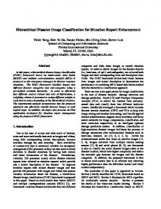
Figure 1.Conceptual model for the prlmary stages in the human Image ~nterpretatlonprocess (for remotely sensed imagery). The order In which features are identified and the rnterrelationsh~psin image cues, objects, image scale, and ancrllary data are not known.

imagery into urban land-use classes. The subject data were then analyzed to define the minimum window size required for correct classification of land-use types. A functional relation between window size and classification accuracy was also constructed. The results of this study suggest that humans require windows of considerably different sizes from what we commonly use in digital image classification studies. Admittedly, this human-centered approach to determining ideal window size for land-use classification is a dramatic departure from the historic methods for researching and evaluating automated classification approaches. It may be argued that we should not design automated image classification logic based on how humans process imagery. This study makes the general assumption that the most efficient and robust automated approaches to image classification (at least for visible wavelength regions of imagery) should be founded on human image interpretation processes. The research context for this work may be illustrated by a conceptual model1 of the human interpretation process with remotely sensed imagery (Figure 1). This simple model reflects three stages in the analysis of remotely sensed imagery under the assumption that the human (1)operates in a manner similar to the instruction found in fundamental air photo interpretation texts, (2) uses the basic image cues of Estes et al. (1983), and (3) identifies intermediate level ab'There is no established conceptual model for how a human actually interprets remotely sensed imagery. This simple model is the author's proposed model.

stractions (or objects) before the final classification. The first stage is the extraction of fundamental spatial image cues, such as texture and pattern, from tone and/or color. This preliminary feature extraction stage has been proposed in the guided search theory (GST) model of Cave and Wolfe (Cave and Wolfe, 1990; Wolfe, 1994) and the feature integration theory of attention model (F'IT) proposed by Treisman and Gelade (1980). The GST and FIT models were proposed by psychologists based on the vision process of general imagery (i.e., non-remotely sensed). In the second stage, intermediate level abstractions (e.g., buildings, trees, etc.) are identified from the fundamental cues and possibly the original tone/ color and feedback from other previously identified abstractions. This second stage of abstractions is what Treisman and Gelade (1980) might argue is focused attention. The cognitive science community, as does the remote sensing community, separates descriptive information about the objects in imagery (i.e., knowledge about such objects) from information extracted directly from the image. Descriptive information about the objects of interest are stored in the human's memory. Such memory resident information is referred to as "top-down" information while information extracted directly from the image is "bottom-up" information. The final classification (e.g., land-uselland-cover categories) is derived from these intermediate objects in the final stage. In a loose sense, the identification of landuselland-cover classes from an agglomeration of intermediate abstractions may be analogous to the "conjunctive search" process proposed in the GST model. Tentative classification of selected portions of the image or

PHOTOGRAMMETRIC ENGINEERING & REMOTE SENSING

objects in the image may become new information available in a feedback loop when examining other image portions or objects. In each of these stages, we may assume that the interpretation analyst requires some minimum amount of local information - the use of a window. If we are to develop automated classification algorithms that produce identical classifications as the human analyst would, we certainly would not expect our automated logic to produce the correct classification if the human could not correctly classify the image. In automated logic, the window defines the portion of an image available for a task - it determines the datalinformation available to the logic. How much datahnformation is needed for accurate classification (i.e., how large should the window be?)? This study probes that question from the perspective of the human analyst.

Background on Window Characteristics Empirlcal Approaches

The window defines the sample size and spatial extent of information of a portion of remotely sensed imagery. A moving window is commonly used in one of three steps of digital image classification: (1) computing features (e.g., texture) in a preclassification stage (Haralick,1972), (2) evaluating neighborhood influences during classification (Swain et al., 19891,and (3) reclassifying pixels in a post-classificationstage (Harris, 1985). Such windows are routinely used on raw spectral data for determining edges or measuring texture. Other studies have used a window to evaluate neighborhood composition or heterogeneity (Murphy, 1985; Fung and Chan, 1994). The window has been used in post-classification studies to "smooth" or remove "noise" for classified maps (Thomas, 1980; Gurney, 1981; Harris, 1985; Bauer et al., 1994; Fuller et al., 1994; Barnsley and Barr, 1996). More recent work in geographic information systems (GISs) has attempted to formalize the language of window operations as local or zonal operators (Tomlin, 1990). The characteristics of the window used in any of the three steps are its size, shape, repetition of application, and the dynamic nature of the sizelshape characteristics in its use. With few exceptions (e.g., Merchant, 1989a; Merchant, i989b; Hodgson, 1991; Dillworth, 1991), the window is treated as square and of fixed size. A number of studies have discussed the problems of boundaries and edges between land-cover categories using a moving window of fixed sizelshape and have suggested alternative solutions (Hsu, 1978; Merchant, 1984a; Merchant, 1984b; Hodgson, 1991; Dillworth 1991; Gong, 1994). In digital image classification, a distinction is made between whether the classification logic uses a per-pixel or an area-based classifier. In a per-pixel classifier, each pixel is uniquely classified using spectral features and more often with additional spatial information from the surrounding area, defined by the window. An area- or region-based classifier would classify all pixels within the window together using spectral and spatial information extracted within the window. Research on determining appropriate measures for characterizing the information content in a window has been conducted since the early 1970s (Figure 2). A number of studies have used a specific size window for evaluating different classification logic or deriving measures of texture, pattern, context, etc. With limited exceptions, previous works with windows in image classification have used the concept of texture for describing spatial variability in brightness values or frequency of classes. Few studies have compared classification results using a range of window sizes PHOTOGRAMMETRIC ENGINEERING & REMOTE SENSING

(Figure 2). It is interesting that most window sizes studied are small - less than a 9 by 9 matrix of pixels. The seminal works on second-order texture statistics by Haralick et al. (1973) were based on windows of 64 rows by 64 columns in size or 20 rows by 50 columns. In this effort, the grey-tone spatial dependency matrix was developed along with 14 fundamental measures of texture from this spatial dependency matrix. Classification of photomicrographs, digitized aerial photography, and Landsat MsS imagery using an area-based classifier resulted in overall accuracies of 89 percent, 82 percent, and 84 percent, respectively. Hsu (1978) examined the difference in classification accuracy of digitized panchromatic aerial photographs using 3 by 3 or 5 by 5 window sizes and 23 texture measures. The ground resolution of the digitized photography examined was approximately 9 m or 1 7 m for the different images. These small window sizes were justified by the interest in detailed landscape information and the problem of "edge effects" from larger windows. Classification accuracies were from 85 percent to 90 percent. Others have used 3 by 3 windows and first-order measures of texture to measure vegetation structure (Cohen and Spies, 1992) and mapping urban environments (Jensen, 1979) in per-pixel classifiers. In a comparison of texture algorithms, Conners and Harlow (1980) examined four texture algorithms and the features of each. A window size of 128 by 64 was used with synthetic imagery in the comparison. Historicallv, texture measures were based on either statistical method; (first-order statistics) or structural methods (second-order measures of texture). More recently, Wang and He (1990) introduced a third method of texture analysis, called the "texture spectrum," based on the frequency of "texture units." Fundamentally, the texture units are based on a 3 by 3 matrix of pixels while the texture spectrum is characterized by the frequency of texture unit values with an n by n matrix of pixels. Using a 30 by 30 matrix of pixels to compute the texture spectrum, the results from a per-pixel classification of four Brodatz natural texture images (Brodatz, 1968) was greater than 95.9 percent accuracy for all four classes. No explanation was provided for the choice of the 30 by 30 matrix size. Wang and He (1990) also provided an example of the separability between three rock units imaged with synthetic aperture radar using a 40 by 40 matrix size with the texture spectrum. No explanation was provided for either matrix size or the ground units associated with the SAR data. A few studies have examined the effects of window size on classification accuracy using per-pixel classifiers. Gong et al. (1992) compared the classification accuracy of three texture measures (statistical, second-order statistics, and texture spectrum) and SPOT multispectral data with window sizes of 3 by 3, 5 by 5, and 7 by 7. A rural-urban fringe landscape was classified into ten Level I1 and six Level I land-use classes. Overall best classification accuracy (Kappa of 0.665) with a single texture measure and the three SPOT bands was with a 5 by 5 window size and the second-order texture measurement. Using a simple first-order statistical measure with a 3 by 3 window size and three SPOT bands resulted in a Kappa of 0.640. The authors indicated that windows larger than 7 by 7 gave unsatisfactory results. In a later study, Gong and Howarth (1992) also attempted to develop a method to predict the optimum size window for deriving texture before the accuracy assessment. In their study, a method for characterizing the grey-level frequencies within a window was introduced. The classification logic used a minimum-distance measure (i.e., Manhattan metric) with the local grey-level frequencies in multiple bands. The classification logic and window selection method

~ u g u s t1 9 9 8

799

128 x 128 TYPE OF STUDY Automated Classification

8

9 $

64x64

PerceptuaVCognitivaClassification

i Indicates a Range in Window j Sires Were Studied

Connem 6 Harloq 19.90.

H o d g m and Uoyd, 19.96

Hemliok. 1973

Haralkk, 1973 a

$/

a0

t

w

j

WanglHe, 1990

Q

3

++

01

I? !/

~gksh#6Ro~19966i

i

:* 11x11

1

9x9

Q

3 Hsu 6 Bu&f

I

.Peddle & Franklin, 1991

0".

+

19

"g ~. : :-

ig /1 :

8 5

0

" 5

19W

., ..

P

/8

,

7x7

,

5x5

.

.. . . .

Z!

I /

i ;

e......

3x 3

lm

/

j

$i

-i si

IDm

Irons 6 Petemon, 1981 i Jensen, 1979 a/

Imns end Peterson, 19.91 .~yhaid & Wwdmck, 1996

.. -.-

20m

40m

60m

SPATIAL RESOLUTION

/

80m

RESOLUTION NOT KNOWN OR NON-R.S. DATA

Figure 2. Previous work in evaluating the use of window size for local spectral operators and its effect on classification accuracy. Few studies have specifically examined a range in window sizes to determine the optimum size. Most work has focused on automated classification logic, while only a couple of studies have tested for cognitive response.

was tested with SPOT multispectral data on an urban-rural fringe landscape. Window size ranged from a 3 by 3 to a 2 1 by 2 1 matrix. Overall, the highest classification accuracy (Kappa of 0.616) was obtained with a 9 by 9 window. However, the authors found that some land-use classes maintained relatively high accuracies as window size increased while other classes decreased in accuracy. Using divergence as a means to determine the optimum size window did not produce satisfactory results. Perceptual/Cognitive Approaches Although there have been perceptual or cognitive studies with imagery in general (e.g., terrestrial scenes from a ground-based observer, interpretation of maps), few studies have focused on remotely sensed imagery collected vertically above the Earth. Research that focused on human cognition related to remotely sensed image interpretation was conducted by Hsu and Burright (1980) and Hodgson and Lloyd (1986) where comparisons were made between the human estimates of texture and the statistical measurements of texture. Hsu and Burright quantitatively assessed the differences in texture of subimages (10 row by 13 column matrices) by 800

A u g u s t 1998

requiring human subjects to estimate the dissimilarity of texture between pairs of choropleth maps. Their study used four choropleth maps (seven gray levels) and ten subjects (cartography students). Although the stimuli for their study were not remotely sensed imagery, their explicit purpose was to extend the relationship between statistical measures of texture and perceptual texture to perceptions of texture to remotely sensed image classification. With some reservations, the authors found that texture may be one dimensional. Hodgson and Lloyd (1986) assessed the human perceptionlcognition of texture using reaction times to indicate the dissimilarity in texture between pairs of subimages. The texture scale for all subimages (64 by 64 in size) was derived from a multidimensional scaling of reaction times. In contrast to Hsu and Burright (1980), in this study a linear scale of texture was indirectly elicited from human subjects. This indirect approach was used to overcome the problem of subjects stating what they think they did when, in fact, their cognitive process may have used other methodslmeasures. Such disagreement between humans verbal descriptions of their process and the actual cognitive processes has been demonstrated in several other studies (Lewicki and Bizot, PHOTOGRAMMETRIC ENGINEERING & REMOTE SENSING

1988; Lundberg, 1988). In the Hodgson and Lloyd (1986) study, the relative difference in texture was determined implicitly using the response time of subjects to every combination of texture images displayed on a CRT screen. The study used ten subimages digitized from panchromatic aerial photography (256 gray levels) and 28 subjects (remote sensing students). In contrast to the work by Hsu and Burright (1980), texture appeared to be clearly one-dimensional. Also, the first-order texture measurements were more strongly correlated to the cognitive scale of texture than were the second-order statistics (e.g., those based on the grey-tone spatial dependency matrix). Despite the strong similarity in cognitive texture and first-order texture measures, it is interesting to note that many automated classification studies favor using second-order texture measures.

Summary of Previous Work

Practically all previous work using windows in either a perpixel or area-based classification logic only implement a square window of fixed size. Evaluation of the effects of window size on classification accuracy has been confined to perpixel classifiers. It is interesting to note that, although the introduction and classical comparisons of texture by Conners and Harlow (1980), Haralick et al. (1973), and Wang and He (1990) used somewhat large windows (i.e., 20 by 50, 64 by 64, and 128 by 64 pixels) for deriving texture measures, the applications of these measures of texture that followed used relatively small windows - 3 by 3, 5 by 5, or 7 by 7 pixels in size (Irons and Petersen, 1981; Jensen, 1996; Gong et al., 1992; Woodcock and Strahler, 1987) . In part, the interest in smaller windows may be due to the negative effects of using large windows, such as for edge effects (Hsu, 1978; Townshend, 1986; Gong, 1994). This focus on small window sizes in previous works may also stem from the desired mapping precision and the spatial resolution of the imagery. Most environmental work and land use projects of urban and suburban landscapes need land unit classification approaching ' 1 4 to '/L acre in size. With the historically available satellite imagery (e.g., SPOT, Landsat) this requires classification approaching the pixel scale. Based on the previous works (primarily per-pixel classification logic), different theoretical curves for the relationship between classification accuracy and window size may be suggested (Figure 3). We might assume that classification accuracy would be highest at small window sizes (e.g., 3 by 3 to 7 by 7 pixels) and would decrease with increasing window size (Figure 3a or 3b). If we follow the examples provided by the authors who introduced the familiar grey-tone spatial dependency matrix (Haralick, 1973) and texture spectrum (Wang and He, 1990), then much larger matrices would be needed (i.e., greater than 20 by 50 pixels). Preliminary work with high spatial resolution imagery by the author suggests that the visual interpreter would also need large window sizes, and the functional relationship may follow a sigmoid curve (Figure 3c). This latter functional relation was also noted in early work by Wharton (1982) with 7.5-m reso-

Variants on Window Characteristics

The window size is generally assumed to be a static, symmetric window, yet other work has advocated various shapes and sizes, and even dynamic windows. Merchant (1984a; 1984b) first suggested the concept of a dynamic geographic window that changes size and shape to fit the application. Analogous to an n by n geometric window that includes the centered pixel and its neighbors, the geographic window includes the "field" (or patch) of interest and the neighboring fields (or patches) of interest. Hodgson (1991) and Dillworth (1991) also argued for a dynamic window size rather than a fixed size window. Hodgson (1991) demonstrated how multiple windows of a variety of shapes and sizes could be used simultaneously to build evidence for characterizing the homogeneity of a landscape. Dillworth (1991) also argued that no one geometric window size provides the best results for any image and suggested an adaptable window that dynamically changes for a given region. It may be that a square window or any regular geometric shaped window is not robust for automated classifications. Dynamic windows that change in shape and size according to some local structure may be more appropriate. The human interpreter may actually use non-geometric and even dynamic windows.

0%

I

3x3

a)

WINDOW SlZE

b)

7x7

25x25

50x50

;

3x3 7x7 25x25

lO0xlW

WINDOW SIZE

c)

50x50

100x100

WINDOW SIZE

LEGEND --_______.__

I~--.~~--~-.-.~~~~~~*

-*

Ernplrlul Form Fmm Pnvlour R.rmrch O a l u n l i u d Thearelied F

m

Figure 3. Theoretical and empirical relationships between classification accuracy and window size for the different land-use/land-cover classes. (a) and (b) suggest classification accuracy is greatest for small window sizes and decreases with increasing window size. (c) suggests that classification accuracy increases monotonically with increasing window size, but in a sigmoid shape. All theoretical functions may be dependent on the spatial resolution of imagery.

PHOTOGRAMMETRIC ENGINEERING & REMOTE SENSING

August 1998

801

lution remotely sensed data, although his classifier operated on biophysical components rather than purely spectral values. The next generation small satellites will have spatial resolutions of 1 m to 3 m for panchromatic bands. For mapping units of ' 1 4 to 1' 2 acre, pixel groups must be classified into land-uselland-cover classes. The nature of spectral information content within a window over such a small geographic area may require a reconsideration of traditional measures of texture, pattern, etc., and the window size. This study focused on the analysis of high spatial resolution imagery that will be available from the next generation small satellites, such as Earthwatch (3m by 3m and l m by lm) and Orbital Sciences ( l m by lm). A range in window sizes were examined with high spatial resolution data to determine which of the functional forms postulated (e.g., Figure 3) best models the performance of a visual analyst.

Methodology The primary considerations in this cognitive study of window size were the experimental design, land-use classification scheme, range in window sizes, image spatial resolution, number of stimuli, and subjects. The stimuli consisted of a random set of subimages, each representing a geometric window of certain extent, extracted from black-and-white aerial photography. The set of subimages represented a range in window sizes. The critical minimum and maximum window sizes would be determined based on the expected improvement and saturation in classification accuracy of these window subimages by a set of subjects (e.g., Figure 3c). It was assumed that the subject would be synergistically using a number of image interpretation elements, such as tone, pattern, texture, shape, size, and association. No attempt was made to determine the relative importance in the interpretation elementsZin the classification of each land use. The assumption was only that the necessary measures of information for correct classification were contained in the respective window size. Eliciting Human Procedures

One method for approaching the problem of selecting an appropriate window size is simply to ask the interpreter "What is the minimum size geometric window necessary to classify this image?" This kind of structured interview is problematic for many cognitive studies, such as the window question, because the subjects may provide an answer for their belief (e.g., "I used a 50 by 50-pixel window") but may be inaccurate when forced to use such a window size. The problem is that humans often have a difficult time articulating processes that are subliminal. Several studies have demonstrated that humans can even "implicitly" learn sequences of graphical patterns or complex relations between elements and subsequently use this learned information yet be unable to articulate the sequences or relations (Lewicki and Bizot, 1988). In fact, when asked to explain one's heuristic, humans often provide justifications of their results rather than descriptions of their method (Lundberg, 1988). A research design can be constructed to subtly tease out this information from human image interpreters. Much work in creating such designs was developed in psychology (Harvey and Gervais, 1981), cartography (Olson, 1979), behavioral geography, and more recently in artificial intelligence (Lundberg, 1989). A key method used in such a research design is the manipulation of the stimuli until a change in the =Asnoted by Estes et al. (1983, p. 933), the basic interpretation elements used in image analysis have not been defined - "...there is not agreement on the number, or the ordering of these elements except at the primitive level." 802

A u g u s t 1998

response is noted. Classification accuracy may be viewed as the subject response. Indicators of a change in response or process are often subjects' answers to questions posed andlor subjects' response times to a question. A correct answer with a faster response time indicates the stimuli added information or was more easily processed by the subjects. In this experiment, the variation in window size was the stimulus manipulated. This study used the correctness in answers as an indicator of response change. For the classification accuracy and window size problem, the expectation was that the function will follow one of the three curves suggested in previous works (Figure 3). However, based on the author's work in human image analysis, interpreters may not be able to correctly classify individual pixels or even very small windows of pixels into Level I1 land-use categories. As the window size increases, the classification accuracy is expected to increase (Figure 3c). It was postulated that the classification accuracy should rapidly increase at some window size and then increase at a decreasing rate as the window size further increases.

Imagery and Classification Scheme A data set of windows of various sizes and land-use classes was collected from black-and-white aerial photography of the Denver, Colorado metropolitan area. The source aerial photography was flown on 15 October 1964 at a scale of 1: 17,400. Earlier work by Welch (1982) recommended a ground resolution in the range of 0.5m to 3m for mapping Level I1 urban land use through visual interpretation. The aerial photography in this study was scanned at a pixel size of 1.5m by 1.5m to insure that all of the Level II classes could be accurately identified in the selected range of window sizes. For this study, the subimages represented Level 11 land-use classes of residential, commercial, and transportation (Anderson et al., 1976) because these are particularly problematic to discriminate between (Jensen, 1979; Jensen, 19961. The desirable range in window sizes included the smallest window where almost n o trained interpreters would be able to identify the land-use classes accurately (Figure 4). The upper end of the window scale would include a size where accurate classification by almost all interpreters would be possible. A preliminary examination of the photography suggested that most trained visual analysts should be able to discern among the three land-use classes with a window approximately 1.5 ha in size. This size area would correspond to a square window on the ground of 122 m by 1 2 2 m (i.e., 80 by 80 pixels of 1.5-m imagery). As a conservative measure, a submatrix of 100 rows by 100 columns (150-m by 150-m ground units) was chosen as the largest size of window. It was expected that even an expert interpreter would have a difficult time correctly discriminating between the land-use classes at window sizes smaller than about 0.20 ha (a 45-m by 45-m square window). Again, a smaller size window of 15 m by 15 m (or a 10- by 10-pixel submatrix) was chosen as a conservative limit (Figure 4). As one may see in Figure 4, accurate classification of the smallest window sizes is exceedingly difficult. The complete set of stimuli consisted of three land-use classes at ten different window sizes. Because the use of only one prototype for a given window size and land-use class may bias the experiment, five different geographical locations for subimages for each land-use class and window size were selected. The window sizes used in the study ranged from a 10 by 10 subimage (15 m by 15 m on the ground) to a 100 by 100 subimage (150 m by 150 m on the ground). Each subsequent window size was 10 rows by 10 columns larger than the previous. Thus, the complete data set consisted of 150 unique subimages. PHOTOGRAMMETRICENGINEERING& REMOTE SENSING

EXAMPLE STIMULI Commercial

Residential

Transportation

Subimage

Geographic Extent

Geographic Area

100 x 100

150m x 150m

2.25ha

135m x 135m

1.82ha

120m x 120m

1.44ha

105m x 105m

l.1Oha

a m

.81ha

II II

.56ha

WB rn

rn

a

1911

rn

30 x 30

e

En

II

ra

BI

E

60m x 60m

.36ha

45m x 45m

.20ha

20 x 20

3om x 3om

.09ha

10 x 10

15m x 15m

.02ha

40x40

REFERENCE SCHEMATIC SUlGLE FAMILY

INTERSTATE

2-Lane Highway

Figure 4. Examples of the range in window sizes for the land-use/land-cover classes of commercial, residential, and transportation. The schematic key representing the relative size of typical features in the urban land-use categories is also shown.

Reproduction To create a large set of these stimuli in this study, the subimages were converted to TIFF format and printed as half-tone images using a high resolution Lineotronics filmwriter. The film output resolution was 1270 dots per inch with a 175line screen. All subimages were enlarged by 220 percent to allow for viewing without the use of magnification lenses. PHOTOGRAMMETRIC ENGINEERING & REMOTE SENSING

(Note: The change in scale does not change the inherent 1.5m spatial resolution of the digital imagery.) The combination of the pixel size at printed scale, line screen, and dot resolution was sufficient to depict the original gray-tone range in the original photography adequately. A random number keyed to each land-use class, subimage, and window size was located outside each window. A u g u s t 1998

803

jects could refer to this schematic during the experiment. The subimages were provided in random order in an envelope. The subject was asked to only pick up and interpret one window at a time, without referring to other previously intermeted imaees. ?he cpesticn asked of each subject was "Is this area predominantly residential, commercial, or transportation?" Each subject was to answer the question for the given window and then write down the random number of the photo subimage with the subimage classification.

Residential Commercial

3

20-

-

0 O

Results rb $Q O; .(ha

r6 rb .She

do

LA

1.0ha

SUBIMAGE SIZE

;o_

L-

2.0ha

-

subimage dimension

ground area

Figure 5. Classification accuracy for each land-use/landcover class as a function of window size. The minimum classification accuracy for each class would be about 33 percent if all subjects randomly selected a class for each windows.

Image Classification A subject pool of 25 undergraduate students who had just completed an aerial photography course was selected. The use of trained students is a common and valid practice used in perceptual/cognitive studies and matches the objectives of this research study. A thorough discussion of the land-use/ land-cover classification system and sample imagery was used to insure the subjects understood the tasks and were competent. Subjects were told that the images were fiom the same series of 1:17,4OO-scale aerial photography of the Denver metropolitan area with which they had previously worked. All subjects had interpreted similar black-and-white aerial photography at the same scale in three different laboratory exercises a month earlier in the course. Thus, each student had a thorough understanding of the definitions of each land-use class as elaborated in the document by Anderson et al. (1976). A small trial dataset consisting of five different subimages was used to orient the subjects to the nature of the experiment and resolve any questions about the tasks. Each student was then given a set of 30 different subimages - ten different window sizes for each of the three land-use classes. No student had the same set of 30 images. A reference schematic depicting the relative scale of a two-lane street, a fourlane highway, a single-family residential home, and a scale bar was given to each subject (bottom of Figure 4). The sub-

Residential committed to.. Window Size

804

A u g u s t 1998

Commercial

Transportation

Because there were only three land-use classes, the minimum expected classification accuracy, by chance, for each class would be about 3 3 percent. In a general sense, the relationship between classification accuracy and window size followed a logarithmic curve rather than an expected sigmoid curve. The classification accuracy for the smalleqt window size (i.e., a 10 by 10) was very poor, ranging from 32 percent for transportation to 54 percent for residential (Figure 5). The accuracy of classification increased immediately for all three land-use classes as window size increased, saturating at about 40 by 40 pixels (60m by 60m). At large window sizes, the accuracy ranged from 88 percent for commercial to 100 percent for residential. There was little variation in accuracy with window sizes larger than 40 by 40 pixels - except for commercial. A more specific examination of the commercial stimuli revealed that certain subimages were more often misclassified than others. In fact, two of the five different commercial subimages at the 90- by 90-pixel window size were misclassified by six of the 25 interpreters. Apparently, due to the nature of commercial land use (such as large homogeneous areas of parking lots or buildings), very large windows are required to encapsulate enough spatial information for accurate classification of some areas. Although the leading tail of the anticipated sigmoid curve was not found, this would be due to the smallest window of only 10 by 10 pixels rather than the common window size in automated procedures of 3 by 3 or 5 by 5 pixels. Such very small window sizes would undoubtedly have been misclassified by the subjects, thus providing the leading tail of the sigmoid curve. An examination of the between-class confusion reveals that the commission errors of residential were generally with commercial and vice versa (Table 1).For instance, the subimages of residential land use that were incorrectly classified were almost always committed as commercial land use. As indicated earlier, the large omission error for 90 by 90 windows of commercial was due to two specific subimages. Misclassified subimages of commercial land use were generally

Commercial commited to.. Residential

Transportation

Transportation committed to.. Commerical

Residential

PHOTOGRAMMETRIC ENGINEERING & REMOTE SENSING

1

committed as residential land use (Table 1).There were almost no commission or omission errors for transportation with window sizes greater than 30 by 30 pixels. Apparently, the unique large linear features associated with the transportation class were easily discernable. The finding that classification accuracy of these Level I1 land uses requires larger windows (greater than 40 by 40 pixels) supports the argument by Merchant (1984a) that small window sizes constrain adequate contextual analysis. The large window size found in this study is also commensurate with the large window sizes used in the seminal works by Haralick (1972), Conners and Harlow (1980), and Wang and He (1990). The implications of these findings are that if the goal in digital image logic is to construct an automated classifier that operates in the same manner as the human, then window sizes should be much larger than the common 3- by 3- or 5- by 5-pixel windows used in automated approaches. It also calls into question the notion of using small windows, regardless of the classification algorithm (e.g., neural network, maximum likelihood, etc.) in classifying land uselland cover from panchromatic, color, or color-IRimagery. If the human cannot correctly classify small subimages, then should we expect an automated classifier to do so? The finding that there is a bias in commission errors by human interpreters may have implications on the use of such reference data and the interpretation of the error matrix for all other remote sensing accuracy assessments and error propagation (Lanter and Veregin, 1992). Treatment of bias in the reference data would require an understanding of the expected biases within the classification scheme used in a specific application. From this study, human-derived classification of Level I1 urban categories is most accurate for residential and transportation and least accurate for commercial.

Discussion The design of the experiment used in this study precludes the use of certain types of information gathered by the human interpreter during many image interpretation applications. For instance, the stimuli were presented to the subjects one at a time, in completely random order, and without visual comparisons between stimuli. In normal circumstances, the photo interpreter may proceed from known to unknown parts of a photograph, thereby using information gained from one part of the scene in classifying other parts of the scene (Stone, 1964). Although the known-to-unknown reasoning could occur within a subimage, the experimental design did not allow it to occur between subimages. The lack of this feedback in the experiment may explain why there was still some classification error at the larger window sizes for commercial and residential. These misclassifications might be avoided in normal interpretation if the interpreter uses the concept of a dynamic window, where the window increases in size to adapt to the local context. Also, the geographic functional linkages (e.g., commercial development along larger transportation corridors) may be better processed by visualizing the entire study area, or at least a larger area than that expressed with the window size range in this study. In fact, the human may be using a hierarchy of windows for the three different stages (Figure I). Either of these concepts that may be at work in visual analysis is problematic to implement in a digital logic. The range in window sizes and spatial resolutions examined in previous work (Figure 2) indicates that few efforts have examined the effects of window size on classification accuracy. To a limited extent, the influence of window size with moderate resolution imagery (e.g., 20 m to 30 m) on automated classification accuracy has been examined. This study has examined the effects of window size (from 10 by PHOTOGRAMMETRIC ENGINEERING & REMOTE SENSING

,001 ha

1.000 ha

WINDOW SIZE (in Ground Area)

Figure 6. Theoretical relationship between image classification accuracy, window size, spatial resolution, and detail of the classification system.

10 to 100 by 100 pixels) on classification accuracy for high spatial resolution imagery (i.e., 1.5 m) and visual classification. The concept of dynamic window sizes and its effect on accuracy for any resolution imagery, using either visual or automated approaches, has not been examined. The relationship between classification accuracy and the use of a specific window size by visual interpreters (a cognitive process) and the spatial resolution of the imagery (a measure of scale) may also vary. This process-scale relation is similar to the notion of changes in the dominant processes as a function of the scale of analysis - a concept well recognized by ecologists (Levin, 1992) and geographers (Meentemyer, 1989). For image analysis, the interpreter may use different cognitive processes in a classification depending on the scale of the imagery. If the human visual process uses window size differently depending on the scale of the imagery, then window size may better be defined as ground area rather than a unitless matrix of pixels. Studies of cognitive processes and studies of automated classification logic should each examine the covariation in spatial resolution and ground area encompassed by a window. If this covariation is understood, then a more robust, and perhaps dynamic, automated classification logic could be designed. It is suggested that a range in sigmoid curves could be used to express the functional relation between classification accuracy and window size, spatial resolution, and specificity of land-uselland-cover classes (Figure 6). Coarser spatial resolution imagery would tend to decrease classification accuracy. However, the overall classification accuracy also depends on the requested specificity in land-uselland-cover categories. In general, it is expected that Level I categories could be classified with higher accuracy than Level I1 categories. Also, classification accuracy may be less with coarser spatial resolution imagery. A change in cognitive process with changes in scale may also suggest that different information measurement logic be used at different image scales. For instance, texture measurement 1 may be better at image scale A while texture measure 2 would be better at scales larger than A. Presuming that the process-scale relation exists, it must still be determined whether the changes in process are linear, nonlinear, or stepped. Finally, the problem of formalizing the process used by the human image interpreter still remains. It is one conclusion to discover the relative window sizes that contain the A u g u s t 1998

805

necessary information content. However, h o w t h e h u m a n determined t h e information from t h e spatial variations i n t o n e w i t h i n t h e w i n d o w i s a major step. It is sometimes a s s u m e d that texture algorithms a n d t h e measures derived f r o m these algorithms adequately describe t h e information content in a subimage for discriminating b e t w e e n other subimages (Conners a n d Harlow, 1980). Visual interpreters m a y u s e a multistage approach (e.g., Figure 1) t o abstract t h e information content w i t h i n a w i n d o w , s u c h a s deriving (1) edges and texture from tonal variation, (2) intermediate objects from contagion, and (3) l a n d u s e from objects. Determining t h e stages in t h e visualization process, cognition of image cues and objects, t y p e of objects a n d object parts, m e t h o d s for associating these objects, a n d feedback between stages, a r e f u n d a m e n t a l t o modeling t h e h u m a n image interpretation process. Additional w o r k b y several researchers using differe n t landscapes c o u l d formalize t h e relations b e t w e e n spatial resolution (scale), w i n d o w size (geographic extent), w i n d o w shape, klassification specificity, a n d classification logics (processes) required t o interpret imagery accurately. For researchers interested i n comparative studies o r for testing other classification logic a n d methods, t h e digital data u s e d in this cognitive s t u d y are available o n t h e Internet a t

http://www.cla.sc.edu/geog/geogdocs/departdocs/facdocs/ hodgson.htm1.

Acknow!edgments T h i s w o r k h a s b e e n s u p p o r t e d i n part b y funding from ERDAS, Inc. a n d NASA-Stennis S p a c e Center, Mississippi. T h e a u t h o r expresses h i s appreciation to James Merchant, J o h n Jensen, Peng Gong, a n d Robert Lloyd for providing a n u m b e r of useful references a n d c o m m e n t s o n a previous draft of this manuscript.

References Agbu, P.A., and E. Nizeyimana, 1991. Comparisons between spectral mapping units derived from SPOT image texture and field soil maps units, Photogrammetric Engineering b Remote Sensing, 57(4):397-405. Anderson, J., E.E. Hardy, J.T. Roach, and R.E. Witmer, 1976. A Land Use and Land Cover Classification System for Use with Remote Sensor Data, Professional Paper 964, United States Geological Survey, Washington, D.C., 28 p. Argialas, D.P., and C.A. Harlow, 1990. Computational image interpretation models: An overview and a perspective, Photogrammetric Engineering b Remote Sensing, 56(6):871-886. Barnsley, M.J., and S.L. Barr, 1996. Inferring urban land use from satellite sensor images using kernel-based spatial reclassification, Photogrammetric Engineering b Remote Sensing, 62(8]: 949-958. Bauer, M.E., T.E. Burk, A.R. Ek, P.R. Coppin, S.D. Lime, T.A. Walsh, D.K. Walters, W. Befort, and D.F. Heinzen, 1994. Satellite inventory of Minnesota forest resources, Photogrammetric Engineering b Remote Sensing, 60(3]:287-298. Cave, K.R., and J.M. Wolfe, 1990. Modeling the role of parallel processing in visual search, Cognitive Psychology, 22:225-271. Chavez, P.A., Jr., and B. Bauer, 1982. An automatic optimum kernelsize selection technique for edge enhancement, Remote Sensing of Environment, 12:23-38. Cohen, W.B., and T.A. Spies, 1992. Estimating structural attributes of douglas-firlwestern hemlock forest stands from Landsat and SPOT imagery, Remote Sensing of Environment, 41(1):117. Conners, R.W., and C. Harlow, 1980. A theoretical comparison of texture algorithms, IEEE Transactions on Pattern Analysis and Machine Intelligence, 2(3):204-222. Dikshit, O., and D.P. Roy, 1996. An empirical investigation of image resampling effects upon the spectral and textural supervised classification of a high spatial resolution multispectral image, Photogrammetric Engineering 6.Remote Sensing, 62(9):10851092. 806

A u g u s t 1998

Dillworth, M.E., 1991. Geographic windows i n remote sensing: Does window size matter?, ASPRS Technical Papers, 1991 ASPRS Annual Convention, 3:122-128. Dutra, L.V., and N.D.A. Mascarenhas, 1984. Some experiments with spatial feature extraction methods in multispectral classification, International Journal of Remote Sensing, 5(2):303-313. Estes, J., E. Hajic, and L. Tinney, 1983. Manual and digital analysis in the visible and infrared regions, Manual of Remote Sensing, Second Edition, American Society for Photogrammetry and Remote Sensing, Falls Church, Virginia, pp. 258-277. Fuller, R.M., G.B. Groom, and A.R. Jones, 1994. The land cover map of Great Britain: An automated classification of Landsat thematic mapper data, Photogrammetric Engineering b Remote Sensing, 60(5):553-562. Fung, T., and K. Chan, 1994. Spatial composition of spectral classes: a structural approach for image analysis of heterogeneous landuse and land-cover types, Photogrammetric Engineering b Remote Sensing, 60(2):173-180. Gong, P., 1990. The use of structural information for improving landcover classification accuracies at the rural-urban hinge, Photogrammetric Engineering b Remote Sensing, 56(1):67-73. , 1994. Reducing boundary effects in a kernel-based classifier, International Journal of Remote Sensing, 15(5]:1131-1139. tual classiGong, P., and P.J. Howarth, 1992. Frequency-based co dentificafication and gray-level vector reduction for landtion, Photogrammetric Engineering b Remote Sensing, 58(4]: 423437. Gong, P., D.J. Marceau, and P.J. Howarth, 1992. A comparison of spatial feature extraction algorithms for land-use classification with SPOT HRV data, Remote Sensing of Environment, 40:137151. Greenfeld, J.S., 1991. An operator-based matching system, Photogrammetric Engineering & Remote Sensing, 57(8):1049-1055. Haralick, R.M., K. Shanmugan, and J. Dinstein, 1973. Textural features for image classification, IEEE Transaction on Systems, Man, and Cybernetics, SMC-3(6):610-621. Harris, R., 1985. Contextual classification post-processing of Landsat data usine a nrobabilistic relaxation model. International Iournal

df

Harvey, L.O., and M.J. Gervais, 1981. Internal representation of visual texture as the basis for the judgement of similarity, Journal of Experimental Psychology, 7(4):741-753. Hodgson, M.E., 1991. Characteristics of the window for neighborhood analysis of nominal data, ASPRS Technical Papers, 1991 ASPRS Annual Convention, 3:206-214. Hodgson, M.E., and R.E. Lloyd, 1986. Cognitive and statistical approaches to texture, ASPRS Technical Papers, 1986 ASPRSACSM Annual Convention, 4:407416. Hoffman, R.R., and J. Conway, 1989. Psychological factors in remote sensing: a review of some recent research, Geocarto International, 4(4):3-21. Hsu, S., 1978. Texture-tone analysis for automated land-use mapping, Photogrammetric Engineering b Remote Sensing, 44(11]: 1393-1404. Hsu, S., and R.G. Burright, 1980. Texture perception and the RADCI Hsu texture feature extractor, Photogrammetric Engineering 6. Remote Sensing, 46(8):151-1058. f 4 Irons, J.R., and G.W. Petersen, 1981. Texture transforms of remote sensing data, Remote Sensing of Environment, 11:359-370. Jensen, J.R., 1979. Spectral and textural features to classify elusive land cover at the urban fringe, The Professional Geographer, 31: 400-409. , 1996. Introductory Digital Image Processing: A Remote Sensing Perspective, Second Edition, Prentice-Hall, Englewood Cliffs, New Jersey. Lanter, D.P., and H. Veregin, 1992. A research paradigm for propagating error in layer-based GIs, Photogrammetric Engineering b Remote Sensing, 58(6):825-833. Levin, S.A., 1992. The problem of pattern and scale i n ecology, Ecology, 73(6):1943-1967. Lewicki, P.T.H., and E. Bizot, 1988. Acquisition of procedural 9

PHOTOGRAMMETRICENGINEERING & REMOTE SENSING

knowledge about a pattern of stimuli that cannot be articulated, Cognitive Psychology, 20:24-37. Lundberg, C.G., 1988. On the structuration of multiactivity task-environments, Environment and Planning A, 20(12):1603-1621. McKeown, D.M., Jr., W.A. Harvey, Jr., and J. McDermott, 1985. Rulebased interpretation of aerial imagery, IEEE Transactions on Pattern Analysis and Machine Intelligence, PAMI-7(5):570-585. Meentemyer, V . , 1989. Geographical perspectives of space, time, and scale, Landscape Ecology, 3(3/4):163-173. Merchant, J.W., 1984a. Using spatial logic in classification of Landsat TM data, Proceedings of the 9th Annual Pecora Symposium, Sioux Falls, South Dakota, pp. 378-385. , 1984b. Employing Spatial Logic i n Classification of Landsat Thematic Mapper Data, Ph.D. dissertation, University of Kansas. Munechika, C.K., J.S. Warnick, C. Salvaggio, and J.R. Schott, 1993. Resolution enhancement of multispectral image data to improve classification accuracy, Photogrammetric Engineering b Remote Sensing, 59(1):67-72. Murphy, D.L., 1985. Estimating neighborhood variability with a binary comparison matrix, Photogrammetric Engineering 6. Remote Sensing, 51[6):667-674. Olson, J.M., 1979. Cognitive cartographic experimentation, The Canadian Cartographer, 16(1):34-44. Peddle, D.R., 'nd S.E. Franklin, 1991. Image texture processing and data i n t k b i o n for surface pattern discrimination, Photogrammetric Engineering b Remote Sensing, 5 7(4):413-420. Pilon, P.G., P.J. Howart, R.A. Bullock, and P.O. Adeniyi, 1988. An enhanced classification approach to change detection in semi-

arid environments, Photogrammetric Engineering & Remote Sensing, 54(12):1709-1716. Ryerd, S., and C. Woodcock, 1996. Combining spectral and texture data in the segmentation of remotely sensed images, Photogrammetric Engineering 6.Remote Sensing, 62(2):181-194. Stone, K.H., 1964. A guide to the interpretation and analysis of aerial photos, Annals of the Association of American Geographers, 31318-328. Thomas, I.L., 1980. Spatial postprocessing o f spectrally classified Landsat data, Photogrammetric Engineering 6.Remote Sensing, 46(9):1201-1206. Tomlin, C.D., 1990. Geographic Information Systems and Cartographic Modeling, Prentice-Hall, Englewood Cliffs, New Jersey. Treisman, A., and G. Gelade, 1980. A feature integration theory of attention, Cognitive Psychology, 12:97-136. Wang, L., and D.C. He, 1990. A new statistical approach for texture analysis, Photogrammetric Engineering 6.Remote Sensing, 56(1): 61-66. Welch, R., 1982. Spatial resolution requirements for urban studies, International Journal of Remote Sensing, 3(2):139-146. Wharton, S.W., 1982. A context-based land-use classification algorithm for high-resolution remotely sensed data, Journal of Applied Photographic Engineering, 8(1):46-50. Wolfe, J.M., 1994. Guided Search 2.0: A revised model of visual search, Psychonomic Bulletin and Review, 1(2):222-238. Woodcock, C.E., and A.H. Strahler, 1987. The factor of scale in remote sensing, Remote Sensing of Environment, 21:311-332. (Received 28 December 1996; revised and accepted 22 January 1998)

C a l l for P a p e r s ~~~

Fourth lntematlonal Alrbome Remote Sensing Conference and Exhlbltlon

-

Development, Integration, Applications & Operations The bddge bemen science and q#idmn 2 1-24 1une 1999

O

~

U

Onbrio, Canada

The Fourth International Airborne Remote Sensing Conference and Exhibition will be held 21-24 June 1999 at the Westin Hotel Ottawa and Macdonald-Cartier International Airport. In addition to a technical program that offers over 350 presentations by experts from more than 35 countries, this unique event will host over 20 airborne platforms including representation from Open Skies Treaty organizations, and over 5 0 exhibitors of remote sensing products and services.

*

Conference Top~cs

+ Environmental Planning, Due Diligence, and Risk Management .) Emergency Situations

.) Atmospheric

and Oceanic Measurements

.) Resource

Management

.) Reconnaissance

Interested contributors should submit a one-page, single-spaced summary, 250 words, by 19 October 1998. Accepted summaries received electronically can be accessed on the World Wide Web before and after the conference.

Written and faxed summaries and inquiries: El Airborne Conference P.O. Box 134008 Ann Arbor, MI 481134008 Telephone: 1-734-994-1200, ext. 3234; Fax: 1-734-994-5123 Inquiries only: [email protected]

Electronic submission: E-mail: [email protected] Website: http://www.eriint.com/CONF/IARSC. html Please provide complete mail/delivery address and facsimile number on all correspondence.

PHOTOGRAMMETRIC ENGINEERING & REMOTE SENSING

+ Airborne Platforms .) Sensors

and Systems Technologies .) Data Handling and Information Product Advancements .) Airborne

and Spaceborne Synergies

A u g u s t 1998

807