When Everyone Runs for the Exit∗ Lasse Heje Pedersen Current Version: August 20, 2009
Abstract The dangers of shouting “fire” in a crowded theater are well understood, but the dangers of rushing to the exit in the financial markets are more complex. Yet, the two events share several features, and I analyze why people crowd into theaters and trades, why they run, what determines the risk, whether to return to the theater or trade when the dust settles, and how much to pay for assets (or tickets) in light of this risk. These theoretical considerations shed light on the recent global liquidity crisis and, in particular, the quant event of 2007.
1
Introduction
People choose to crowd into a theater or a trade because they share a common goal: in one case, they all want to see the best play in town, in the other, they all pursue the highest risk-adjusted return. They run for the exit because staying is associated with real risk, namely being caught in the theater fire or being forced to liquidate at the most distressed prices. Many people running introduces a second, and endogenous, risk: Theater guests risk being trampled by running feet, and traders risk being trampled by falling prices, margin calls, and vanishing capital — a negative externality that increases the aggregate risk. The risk of running for the exit depends on how crowded the theater or trade is, and the quality of risk management. The liquidity risk can be reduced by restricting ∗
I am grateful for helpful comments from Yakov Amihud, Jacob Bock Axelsen, David Backus, Markus Brunnermeier, Jennifer Carpenter, Douglas Gale (the editor), Arvind Krishnamurthy, Bill Silber, and Jeff Wurgler, as well as from participants at the Inaugural Financial Stability Conference on Provision and Pricing of Liquidity Insurance hosted by the International Journal of Central Banking and the Federal Reserve Bank of New York. This paper has benefitted from the insights gained at AQR Capital Managements, including from Michele Aghassi, Cliff Asness, Ronen Israel, Toby Moskowitz, Lars Nielsen, and Humbert Suarez. The author is at New York University, CEPR, and NBER, 44 West Fourth Street, NY 10012-1126; e-mail:
[email protected], http://www.stern.nyu.edu/∼lpederse/.
reliance on funding that cannot be depended on during crises, by limiting how large and levered positions one takes, or, even better, if the leveraged players limit how large an aggregate position they take relative to their capital. Finally, investors return to these markets as liquidity crises create opportunities. Indeed, the expected return on liquidity provision rises during crisis. Just like fear of a theater fire would reduce ticket prices, liquidity risk reduces asset prices. A panic run to the exit is so dangerous that Justice Oliver Wendell Holmes Jr.’s opinion in the U.S. Supreme Court’s decision in Schenck v. U.S. (1919) states: “The most stringent protection of free speech would not protect a man falsely shouting fire in a theater and causing a panic.” Panic runs have been studied extensively by physicists,1 who document and model how people try to move faster and start pushing, passing of bottlenecks becomes uncoordinated, exits are clogged, alternative exits are used inefficiently, and the risk depends on the design of the exit routes. As evidence of the danger of such runs, jammed crowds can cause pressures up to 4500 Newtons per meter, which can bend steel barriers or tear down brick walls, and escape is further slowed by fallen or injured people turning into “obstacles.” A panic run in the financial markets is also serious, and, indeed, the global crisis that started in 2007 provides ample evidence of the importance of liquidity risk. Subprime credit losses put highly levered financial institutions into a tailspin, their sources of funding dried up, and each institution’s liquidations and risk reductions added stress to the other institutions as the crisis spilled over to other credit markets, money markets, currency markets, convertible bonds, stocks, and over-the-counter derivatives. Central banks’ balance sheets increased significantly as they tried to address the funding problems using various lending programs and unconventional monetary policy tools. I focus on the “quant” event of August 2007 as it illustrates well the nature of liquidity crises. While this event was almost invisible to the public, it can be seen very clearly through the lens of a diversified long-short strategy. Quantitative traders running for the exit had a significant impact on some of the most liquid markets in the world, and I show how prices dropped and rebounded in early August 2007. Using high-frequency data, I document an amazing short-term predictability and volatility driven by the run to the exit (Figure 1, Panel (a)). In hindsight, the quant crisis was an early warning signal of how the levered system would face trouble as the liquidity spirals caused havoc in the global markets. The recent liquidity crisis is the last in a string of earlier ones throughout history, such as the crash of 1987, the crisis following the Russian default in 1998, the convertible bond episode in 2005, and currency crashes when carry trades unwind. To reduce the risk of the next one, it is important to understand the mechanisms that drive these crises. Therefore, after presenting the evidence from the global liquidity crisis and the 1
See Helbing, Farkas, and Vicsek (2000), Helbing (2001), Helbing, Buzna, Johansson, and Werner (2005), and references therein.
2
Panel (a): Minute-by-Minute Data from the Quant Event 2007. 5.00%
0.00%
-5.00%
-10.00%
-15.00%
-20.00%
-25.00%
-30.00% 20070803 09:31:00
20070806 09:31:00
20070807 09:31:00
20070808 09:31:00
20070809 09:31:00
20070810 09:31:00
20070813 09:31:00
20070814 09:31:00
Panel (b): Theoretically Predicted Price Path 118
116
114
112
price
110
108
106
104
102
100
98 4.5
5
5.5
6
6.5
7
time
Figure 1: Everyone Runs for the Exit. Panel (a) shows the cumulative return to a long-short market-neutral value and momentum strategy for U.S. large cap stocks, scaled to 6% annualized volatility during August 3-14, 2007. Panel (b) illustrates the Brunnermeier and Pedersen (2005) model’s predicted price path when everyone runs for the exit.
3
quant event in Section 2, I consider some models of liquidity risk in Section 3.2 I analyze the underlying causes of forced selling, the reasons why other investors may sell even if they are not forced to do so, and the resulting price path (Figure 1, Panel (b)). I show how “liquidity spirals” amplify and spread the initial shock when selling leads to more selling, higher margin requirements, tighter risk management, and withdrawal of capital, consistent with the evidence from the crisis that I present. Finally, I discuss the implications for asset pricing and monetary policy. I explain how securities with larger and more varying transaction costs must offer higher expected returns as compensation for the larger market-liquidity risk. Further, securities with higher margin requirements must offer higher expected returns as compensation for their larger use of capital and funding-liquidity risk. For instance, securities backed by loans and other credit instruments have higher yields (or lower prices) if their market liquidity risk and margin requirements are higher. Hence, monetary policy that affects margin requirements (or “haircuts”), funding, and market liquidity can thus affect asset prices and credit availability.
2
Running for the Exit in the Real World
I first study the recent global financial crisis and how it spilled over across asset classes with a special focus on the quant event of August 2007.
2.1
The Global Liquidity Crisis that Started in 2007
In the years preceding the crisis, the global financial markets were flush with liquidity due to low interest rates, high savings rates in Asia, economic growth, and low volatility. As a response to low borrowing costs and low apparent risk, financial institutions became highly levered (a positive liquidity spiral). This made them vulnerable. When house prices started to decline and it started to become clear in 2007 that subprime borrowers would default in large numbers, an adverse liquidity spiral was kicked off. Many banks experienced significant mark-to-market losses, and two hedge funds at Bear Stearns blew up due to subprime-related collateralized debt obligations (CDOs) in June 2007. Market liquidity dried up in one market after another as volatility picked up, funding became tight, and risk premia rose as seen in Figure 2. The figure shows the evolution of market liquidity as measured by bid-ask spread, in percent of mid quote, averaged across large cap U.S. stocks.3 The figures also shows the TED spread and the 2
My understanding of the crisis is largely based on my own research, and this is reflected in this note. Amihud, Mendelson, and Pedersen (2006) review the broad literature on liquidity and asset pricing, and Gorton (2008), Brunnermeier (2009), and Krishnamurthy (2009) review the crisis and amplification mechanisms. 3 This is computed using tick data, using the best bid and ask quotes at 3PM each day.
4
VIX index. The TED spread is the difference between the interest rate on 3 months uncollateralized interbank LIBOR loans and the interest rates on Treasury Bills. A high TED spread indicates reluctance to provide interbank loans, that is, risks and funding problems in the financial sector. VIX is the volatility of the S&P500 equity index as implied by the option markets, and may also be related to funding liquidity as many financial institutions are exposed to the VIX directly or indirectly. We see that there is a close co-movement between bid-ask spreads and VIX throughout the crisis, and also a visible connection to the TED spreads, indicating a link between market liquidity, funding liquidity, and volatility as explained by the theory in Section 3.4 6 Bid-Ask VIX TED
5
4
3
2
1
0
-1
-2 07-2006
11-2006
03-2007
07-2007
11-2007
03-2008
07-2008
11-2008
03-2009
07-2009
Figure 2: Bid-Ask Spreads During the Global Liquidity Crisis. The chart shows average bid-ask spread for large cap U.S. stocks, the equity volatility index VIX, and the interest-rate spread between LIBOR and Treasury bills (TED) from July 2006 to July 2009. Each of the series has been scaled to have a zero mean and a unit standard deviation.
4
See Nagel (2009) for further evidence.
5
2.2
Spirals and Spillover
The shock to the subprime credit market spread quickly spilled over to other markets as seen in Figure 3. It spread to credit markets more broadly, to money markets, to quant equity in the U.S., and later to quant equity in Japan and beyond. Next, the liquidity shock started to affect the currency carry trade, commercial mortgage backed securities, convertible bonds, event arbitrage, and fixed-income markets. Investors ran for the exit in one market after another, and the rush to the exits reached its peak after Lehman failed in September 2008. Market liquidity deteriorated in most markets and vanished almost completely in many over-the-counter markets. For instance, dealers in emerging-market interest-rate swaps largely stopped quoting bid and ask prices. The extreme market liquidity risk was complemented by extreme funding liquidity risk as haircuts and margin requirements went up and certain securities became unacceptable as collateral for many counterparties. As the funding situation for banks and other financial institutions deteriorated, central banks globally had to expand their balance sheets substantially to deal with the ramifications. In many different markets, it turned out that levered liquidity-providing traders had some common features in their portfolios. Despite their different investment philosophies and analysis, one manager’s long positions was another manager’s long more often than it was a short. Is this herding in the sense that traders are buying something because they have heard that others are buying it? It need not be. Consider the theoretical benchmark of each trader doing his independent analysis on common data: in a standard Markowitz/CAPM world, all investors are holding exactly the same portfolio, namely the “tangency” portfolio with the highest risk-adjusted return. While real-world traders are far more diverse than this theoretical benchmark since they use different methods to estimate risk and expected return, it is natural to expect that at least the most sophisticated traders in a specific market have some overlap in their portfolios since they are striving towards the same goal.
2.3
What is Quant?
Before showing more detailed evidence from the quant event, it is useful to briefly explain what quant is. Most traders, e.g. proprietary traders and hedge funds, engage in “discretionary trading,” meaning that the decision to buy or sell is at the trader’s discretion given his overall assessment based on experience, various kinds of information, intuition, etc. This traditional form of trading can be seen in contrast to “quantitative trading,” or “quant” for short.5 Quants define the trading rules explicitly and build systems that 5
Quantitative traders are close cousins to, but perform different roles than, the “sell-side quants” described in Emanuel Derman’s interesting autobiography “My Life as a Quant”. Sell side quants provide analytical tools that are helpful for hedging, risk management, discretionary traders, clients,
6
110.00
100.00
90.00
80.00
70.00 Subprime AA ABX Quant US Quant JP Currency Carry
60.00
7
7
/0 26 8/
8/
19
/0
/0 12 8/
5/ 8/
29 7/
7
07
7 /0
/0 22 7/
7/
15
/0
7
7
07 8/ 7/
7/
1/
07
50.00
Figure 3: Spillover in the Beginning of the Crisis (July-August, 2007). The figure shows how the crisis started with a decline in the price of the subprime credit. In July 2007, quantitative long-short stock-selection strategies based on value and momentum in the United States (Quant US) began to experience losses, and subsequently this spilled over to similar strategies in Japan (Quant JP). The currency carry trade experienced an unwinding in the end of August. The price series and cumulative returns have been normalized to be 100 in the beginning of July.
implement them systematically. They try to develop a small edge on each of many small diversified trades using sophisticated processing of ideas that cannot be easily processed using non-quantitative methods. To do this, they use tools and insights from economics, finance, statistics, math, computer science, and engineering, combined with lots of data (public and proprietary) to identify relationships that market participants may not have incorporated in the price immediately. They build computer systems that generate trading signals based on these relationships, perform portfolio optimization in light of trading costs, and trade using automated execution schemes that route hundreds of orders every few seconds. In other words, trading is done by feeding data and other purposes.
7
into computers that run various programs with human oversight. Some quants focus on high-frequency trading where they exit a trade minutes or days after it was entered. Others focus on lower frequency trades, and still others do some of both. For instance, “value” strategies seek to buy cheap securities (and short over-valued ones), and, since such securities often stay cheap for months, this is a low frequency (that is, low turnover) strategy. “Momentum” strategies buy securities that recently performed relatively well, while shorting under-performing securities, based on the idea that such recent performance has tended to continue more often than it has reversed. (Value and momentum in many asset classes is discussed in Asness, Moskowitz, and Pedersen (2008)). Another strategy is to provide liquidity to securities with temporary order imbalances that are associated with short-term price reversals, and this is inherently a high-frequency strategy. While discretionary trading has the advantages of a tailored analysis of each trade and the use of soft information such as private conversations, its labor-intensive method implies that only a limited number of securities can be analyzed in depth, and the discretion exposes the trader to psychological biases. Quantitative trading has the advantage of discipline, an ability to apply a trading idea to a wide universe of securities with the benefits of diversification, efficient portfolio construction, and an ability to “back test” the strategy, meaning that one can check how well one would have done by following such a strategy in the past. Of course, past success does not guarantee future success, but at least it rules out using rules that never worked and, to a degree, psychological biases. The quant method’s disadvantage is its reliance on hard data and the computer program’s limited ability to incorporate real-time human judgment.
2.4
The Quant Event of August 2007
Quants trade in many markets and, in particular, take significant long and short positions in stocks. By mid-2007, quant-managed stock portfolios had about 300-400 billion dollar long and short positions in equities by some estimates. In August, a significant liquidity event occurred in which some quants were forced to unwind and others also reduced positions. The buying and selling pressure was immense. It consisted of hundreds of billions of dollars as aggregate positions were reduced approximately by half according to some prime broker estimates. While the effects were clear to quants, they were at first largely hidden to outsiders since the trades were spread over thousands of stocks, with some stock prices being pushed up and others pushed down. To “see” the event, one must look through the lens of a typical quant’s diversified long/short portfolio at a high frequency. While the precise origin of the event is hard to determine with certainty, the following is a likely sequence of events (see also Khandani and Lo (2007) and Khandani and Lo (2009)). In June 2007, many banks and some hedge funds experienced significant losses due credit exposure or to the ripple effects of the credit turmoil. In 8
July, some started to reduce risk and raise cash by selling liquid instruments such as their stock positions, hurting the returns of common stock-selection strategies. Some banks even closed down some of their trading desks down, including quant proprietary trading operations. Simultaneously, some hedge funds were experiencing redemptions. For instance, some funds of funds (hedge funds investing in other hedge funds) hit loss triggers and were forced to redeem from the hedge funds they were invested in, including quants. The quant value strategy in particular experienced losses in July. Money was pulled out of stocks that were potential leveraged buy-out (LBO) candidates because of the reduced access to leverage. These were stocks that LBO firms considered cheap based on strong value and cash flow characteristics, and, since quants typically consider similar characteristics, this hurt value strategies. Value strategies were also hurt because the cheap stocks on the long side had more leverage and therefore more sensitivity to widening credit spreads. On Monday August 6, 2007 a major de-levering of quant strategies began. Figure 1, Panel (a) shows the cumulative return to a industry-neutral long-short portfolio based on value and momentum signals. We see that the portfolio incurs substantial losses from Monday, August 6 through Thursday, August 9, as quants were unwinding, and then recovers much of its losses on Friday and Monday as the unwinding ended and some traders may have re-entered their positions. The smoothness of the graph is noteworthy. It is not an artifact of drawing the graph by connecting a few dots – the graph uses minute-by-minute data. The smoothness is due to a remarkable short-term predictability arising from the selling pressure and subsequent snap back. For instance, on Tuesday August 7, the strategy was down 90% of the ten-minute intervals, and it was up 75% of the ten-minute intervals on that Friday. This predictability provides strong evidence of a liquidity event as it is statistically significantly different from the behavior of a random walk. Another striking feature of the graph is the sheer magnitude of the drop and rebound. The strategy has been scaled to have an annualized volatility of about 6% using a well-known commercial risk model. The strategy loses about 25% in four days, about 4 annual standard deviations and more than 30 standard deviations based on the 4-day volatility of (4/260)1/2 ∗ 6% = 0.74%. The 30 standard deviations must be interpreted correctly. This number does not mean that this was a thousand year flood and can never happen again. It means that the event was a liquidity event, not based on stock fundamentals, and that this risk model does not capture liquidity risk and the endogenous amplification by the liquidity spirals. Stock price fluctuations are driven primarily by economic news about fundamentals most of the time, but during a liquidity crisis, price pressure can have a large effect. Hence, the distribution of stock returns can be seen as a mixture of two distributions: shocks driven by fundamentals mixed with shocks driven by liquidity effects. Since fundamentals are usually the main driver, conventional risk models are calibrated to capture fundamental shocks and liq9
uidity tail events are not well captured by such models. Hence, 30 standard deviations means that the event is statistically significantly different from a fundamental shock, and, hence, must have been driven by a liquidity event. The quant event started with the U.S. value strategy and spilled over to global markets, e.g. Japan as seen in Figure 3, and to certain other types of quant factors, though not all. For instance, even though momentum is normally negatively correlated to value, these strategies became positively correlated as they both experienced significant losses during the unwind. Also, certain high-frequency strategies that rely on price reversals were affected due to the unusual amount of price continuation. It is curious to notice the resemblance between the actual data from 2007 in Panel (a), and the price path in Panel (b) predicted by the Brunnermeier and Pedersen (2005) model that we discuss next: Both graphs go down smoothly, go back up smoothly, and, finally, level off below where they started.
3
Theoretical Background
To understand the mechanisms that drive liquidity crises, I first consider a stylized model of running for the exit. I then show how endogenous systemic liquidity risk arises as agents run for fear of being trampled, and, lastly, discuss the asset pricing implications.
3.1
Running for the Exit
There are two “arbitrageurs,” and we seek to model the notion that they might run for the exit using a simplified version of the model of Brunnermeier and Pedersen (2005). They trade with each other and with a group of “long-term traders”, who in the aggregate give rise to a demand curve with a slope of 1. In order words, if the arbitrageurs buy one share, the equilibrium price goes up by 1, and, if they sell one share, the price drops by 1.6 The agents trade at times 0, 1, and 2, and the asset pays off its dividend at the final time 3. The arbitrageurs can hold at most 10 shares due to limited capital and margin constraints. At time 0, the arbitrageurs each buy 8 shares since their information indicates that the asset is undervalued at its price per share of, say, 116. For simplicity, we take the size of this initial purchase as given, but Brunnermeier and Pedersen (2005) show how it can be derived as an optimal trade-off between potential liquidation costs (discussed below) and the benefits of buying an undervalued asset early. The arbitrageurs have 6 Evidence on downward sloping demand curves in provided by Shleifer (1986), Wurgler and Zhuravskaya (2002), and others.
10
similar positions because they are looking for the same thing, namely securities that offer high returns. At time 1, one of the arbitrageurs might lose money in another trade (say, subprime debt) which forces him to sell his entire position of 8 shares in the asset under consideration, or, alternatively, neither arbitrageur suffers such a shock. In case neither suffers a shock, both arbitrageurs buy 2 additional shares to be fully invested up to their limit, which pushes the price to 116+2+2= 120, where it stays until the final dividend is paid at time 3 (a dividend which the arbitrageurs expect to be above 120). Let us consider the more interesting case where one arbitrageur is distressed and is forced to sell. Suppose first that the other arbitrageur doesn’t trade anything at this time (e.g., because he does not know about the other arbitrageur’s distress). In this case, the distressed selling pushes the price down to 116-8=108 for an average execution price of 112. What if the other arbitrageur knew that this selling pressure was coming? Then he would be able to predict that the price would drop and, as a result, that he would incur a mark-to-market loss. Therefore, he would optimally also sell at time 1, and buy back his position at time 2. The price path associated with this selling followed by buying is illustrated in Figure 1, Panel (b). Since both traders are selling at time 1, the price drops from 116 to 116-8-8=100 with an average execution price of 108. When the non-distressed trader is buying back his 8 shares at time 2, he pushes the price back up to 100+8=108 with an average execution price of 104, and he then buys 2 additional shares, pushing the price to 110. Importantly, given that he sold for 108 on average and bought back at 104, his wealth is 4 dollars higher than if he had not traded. The drop and rebound in prices resembles that of the quant event (Panel (a)) and other liquidity events, and it means that the distressed trader’s losses are worsened. When he liquidates alone, he receives an average execution price of 112, but, with both selling, the average execution price is 108 since the price drops more sharply (and he does not enjoy the rebound that happens after he is out of the market). If the other trader manages to sell before the distressed trader (frontrunning) then the distressed trader would realize an even lower liquidation value. Hence, the distressed trader rushes to the exit as fast as he can. In fact, both arbitrageurs run for the exit and this exacerbates the distressed traders’ losses. In this simple example, the non-distressed trader sold and bought back to enhance his overall profit in the long run. However, the real world is more complex than that. If someone else is pushing down the price of the assets you hold, you could soon become distressed yourself. Brunnermeier and Pedersen (2005) consider this endogenous distress and show that there can be multiple equilibria: “panics” can occur when people sell because they fear others will sell, leading to more failures than in equilibria where traders stay “calm.” In a panic equilibrium, the traders thus “step on” each other as they run for the exit. This leads to systemic risk: a fear of forced selling leads to 11
selling, and selling leads to forced selling as discussed further in the next subsection. We have seen that liquidity evaporates exactly when it is most needed in this setting, but, with more than one non-distressed trader, will competitive forces ensure that the price is at its efficient level? The answer is: not generally, since running for the exit occurs even with multiple traders in this setting. Could this be because there are only a few time periods? In other words, since the non-distressed traders ultimately want to hold this position, why don’t they compete in being the first to buy back the position in a way that makes the price stabilize without overshooting? Brunnermeier and Pedersen (2005) address this by allowing many trading opportunities in a continuous-time model and show that this competition does in fact occur if the non-distressed traders have enough excess capital to absorb the shares that the distressed traders need to sell.7 However, if the non-distressed traders don’t have enough capital to absorb all these shares, then the price must ultimately fall, and this price drop gives an incentive to sell early (at a high price) and buy back later (at a low price), leading to price overshooting. Hence, running for the exit happens only when the selling pressure is large relative to the available capital on the sideline. Said differently, it happens when the trade is crowded and a significant part of the crowd is near or over the edge, with few “outsiders” ready to step in (e.g., because it takes time to build the expertise and infrastructure to trade these assets). In related work, Carlin, Lobo, and Viswanathan (2008) consider a model in which traders cooperate most of the time due to repeated interaction, but episodic liquidity crises occurs. Chu, Lehnert, and Passmore (2009, this issue) extend the framework to multiple assets and consider cross-asset effects and possible interventions. Duffie, Gˆarleanu, and Pedersen (2007) consider a funding shock among a group of investors in an over-the-counter search market and show how the speed of the drop-and-rebound price signature depend on the market liquidity. In illiquid markets with time-consuming search, the drop-and-rebound occurs over a longer time period and with a deeper drop in prices. Lagos, Rocheteau, and Weill (2007) model dealers’ liquidity provision following a crash.
3.2
Running for Fear of Being Trampled: Endogenous Liquidity Risk
It is interesting to dig a level deeper into the main drivers of forced selling and the mechanisms that make the run spiral into a panic liquidation. As illustrated in Figure 4, suppose an initial shock (a shout of “fire”) leads to losses of traders, e.g. subprime losses due to a dropping house prices as in the most recent liquidity crisis. Traders 7
Figure 1, Panel (b) is in fact from a continuous-time example in that paper (the numbers in the discrete-time example above are chosen so the examples match).
12
then reduce their positions, which pushes prices away from fundamentals, and liquidity spirals make the effect dis-proportionally larger than the initial shock. This endogenous liquidity risk has several key elements: First, as prices move away from fundamentals, the market becomes illiquid, volatility picks up, and these effects make it riskier for others to finance the trader’s positions. Therefore, margin requirements (or haircuts) increase, and, in extreme cases, counterparties refuse to lend against certain securities as collateral. For instance, after Lehman’s failure in September 2008, it became difficult to borrow against certain illiquid fixed-income securities. High margins and inability to finance positions naturally worsens levered traders’ funding problems, leading to further selling, and so on as the margin spiral swirls (Brunnermeier and Pedersen (2009)). The second effect is that prices start moving against the liquidity-providing traders’ positions, leading to losses, inducing further unwinding, and the losses spiral. This is worsened if poor performance leads to further reductions in capital, for instance if a hedge fund has redemptions, or a bank (or multi-strategy hedge fund) moves capital away from one trading desk to use it elsewhere (Shleifer and Vishny (1997), Xiong (2001), Gromb and Vayanos (2002), Vayanos (2004)). Thirdly, many traders’ risk management tightens at these times since volatility increases — especially the volatility measured over a possible liquidation period which lengthens due to illiquidity — and one trader’s prudent risk management can be an other trader’s vanishing market liquidity and funding. As risk management tightens, traders sell to reduce risk and banks cut back the funding they provide, leading to further funding problems, and a risk management spiral arises (Garleanu and Pedersen (2007)). Portfolio insurance is an extreme example of this, and stop-loss orders is another example. Further, when banks face losses, depositors may withdraw capital to limit their risk, other creditors may not roll over debt, counterparties shy away, and this can lead to a bank run (Diamond and Dybvig (1983), Holmstrom and Tirole (1997), Allen and Gale (2007), Acharya, Gale, and Yorulmazer (2009)). Figure 2 shows how market liquidity, funding liquidity, and volatility spiraled in the liquidity crisis that started in 2007. Mitchell, Pedersen, and Pulvino (2007) document how these liquidity spirals played out in the convertible bond market in 1998 and 2005, and in the merger market in 1987. Similar – and, in fact, larger – liquidity spirals have caused havoc in the convertible bond and fixed-income markets during the recent crisis. Brunnermeier and Pedersen (2009) discuss how the interplay between market liquidity and funding liquidity can help explain commonality in liquidity across securities and markets, flight to quality, that liquidity is poor in down markets, and other empirical phenomena documented by Chordia, Roll, and Subrahmanyam (2000), Hasbrouck and Seppi (2001) and Huberman and Halka (2001), Coughenour and Saad (2004), Chordia, Sarkar, and Subrahmanyam (2005), Hameed, Kang, and Viswanathan (2005), and Hendershott, Moulton, and Seasholes (2006). Adrian and Shin (2009) provide evidence that broker-dealers have pro-cyclical leverage, consistent with the 13
reduced positions
initial losses e.g. due to credit
prices move away from fundamentals
funding problems
higher margins losses on existing positions tighter risk management
Figure 4: Liquidity Spirals. The chart shows how an initial shock to financial institutions’ funding is amplified by increasing margins (margin spirals), losses on existing positions (loss spiral), and tightened risk management (risk management spiral).
margin spiral. Brunnermeier, Nagel, and Pedersen (2008) document that speculators use the carry trade in currency markets, and their unwinding during funding crises leads to currency crash risk. The crash risk discourages speculators from taking large enough positions to enforce the uncovered interest-rate parity (UIP), and thus funding liquidity risk can help explain the forward premium puzzle.
3.3
Implications for Asset Pricing
Given the costs incurred in liquidity crises, investors must manage their liquidity risk and be compensated for taking on liquidity risk. Hence, securities with more liquidity risk must offer a higher return to compensate investors for incurring the risk. Acharya and Pedersen (2005) consider such a model in which transaction costs change unpredictably over time.8 Since investors care about return net of costs, the CAPM holds in net returns. A security’s required return depends, therefore, on its net-return i M i beta, that is, the covariance covt (rt+1 − cit+1 , rt+1 − cM t+1 ) between the return r net of trading costs ci with the market return rM net of market trading costs cM . This covariance can be separated into four terms, namely the standard market beta coming i M from covt (rt+1 , rt+1 ) as well as three liquidity risks: (i) +covt (cit+1 , cM t+1 ) is the compen8
Amihud and Mendelson (1986) show how required returns depend on average market liquidity.
14
sation for the commonality of liquidity as investors require higher returns for securities with higher trading costs during liquidity crises when trading costs are high in general; i (ii) −covt (rt+1 , cM t+1 ) with a negative sign, meaning that investors require higher return for a security that has a low return during liquidity crises when cM is high; and (iii) M ) implying compensation for high illiquidity in a down market. −covt (cit+1 , rt+1 This market-liquidity-adjusted CAPM implies that, when the market becomes illiq∂ i f uid and liquidity risk goes up, the required return rises ( ∂C i Et (rt+1 − r ) > 0) and, t i therefore, contemporaneous returns are low (covt (cit+1 , rt+1 ) < 0). For instance, due to the liquidity risk that arose when the banking system faced trouble in 2008, the required return rose, which contributed to the downfall in prices. Amihud (2002), Pastor and Stambaugh (2003), and Acharya and Pedersen (2005) find empirical evidence for the pricing of liquidity risk. Garleanu and Pedersen (2009) consider the asset pricing effects of funding liquidity risk — as opposed to market liquidity risk discussed above — by showing how a security’s margin requirement can increase its required return.9 The paper considers a relatively minimal extension of the Lucas tree model, having two groups of agents with different risk aversion facing margin requirements. The more risk tolerant agents (which can be interpreted as the financial institutions) use leverage. Hence, after negative fundamental shocks, they incur large losses and ultimately hit their margin constraint. The paper shows that a security’s required return is the sum of its beta times the risk premium (as in the standard CAPM or consumption CAPM), and its margin requirement times the cost of capital — a compensation for funding liquidity risk. The paper finds large asset pricing effects by explicitly solving the model and calibrating it using realistic parameters, and the model can help explain the deviations from the Law of One Price during the recent and previous crises. For instance, corporate bonds have traded at higher yield spreads than corresponding credit default swaps (CDS), giving rise to an apparent arbitrage called the CDS-bond basis. This can be explained by the fact that the margin requirement on the bond is higher than that of the CDS. Hence, investors require a higher yield on a high-margin bond than on a low-margin CDS when capital is scarce. Further, the basis varies in the time series with the tightness of credit and in the cross section with the margin differential, consistent with the model. Another stark failure of the Law of One Price is the failure of covered interest-rate parity (CIP), which was driven by a dollar funding need by global financial institutions combined with a limited ability to arbitrage the deviation due to binding margin requirements. The Fed and other central banks have tried to improve the financing environment by providing lending programs that offer collateralized loans with lower margins than 9
He and Krishnamurthy (2008) consider a model where intermediaries are constrained in raising equity instead of debt.
15
otherwise available. Since lower margins lead to lower required returns, this leads to higher prices of debt securities, which ultimately results in improved credit conditions for businesses and households. Ashcraft, Garleanu, and Pedersen (2009) use a survey conducted by the Fed to see how market participants change their bids in response to lower margins/haircuts. The evidence suggests that the effect of margins is very large. Margins, and financing conditions more broadly, are important both for asset prices and for financial firms’ ability to operate, and these affect the real economy through consumers’ and firms’ access to credit and ability to issue securities. Hence, lending programs, broadening the acceptable collateral, and setting margins/haircuts are important monetary policy tools during liquidity crises.
4
Conclusion
The recent liquidity crisis’ severe consequences for the global economy highlight the importance of liquidity risk. Liquidity shocks are sudden, spill over across markets where levered traders have positions, and affect mostly risky and illiquid securities with large increases in margins. Liquidity events can happen even in the most liquid markets in the world as clearly illustrated by the sharp drop and rebound in the values of quant positions in U.S. large cap stocks during August 2007. Investors need to manage both their funding liquidity, including their cash management, the financing terms (margins/haircuts), and the risk of changes in financing or equity redemptions, and their market liquidity risk, including the trading costs, possible hikes in trading costs, the time it takes to unwind positions in an orderly fashion, and the risk of predatory trading (Brunnermeier and Pedersen (2005, 2009)). Further, investors need to be compensated for taking liquidity risk. Their pricing models should capture market liquidity risk (Acharya and Pedersen (2005)) and funding liquidity risk (Garleanu and Pedersen (2009)). While predicting liquidity crises in advance is very challenging, it is useful to understand whether price drops that already occurred were due to liquidity or fundamentals. This is because liquidity events present both risks and opportunities — liquidity induced price drops tend to revert and investors with dry powder can try to capture this rebound. During a liquidity crisis, central banks can use unconventional monetary tools that improve the financing environment, e.g. by offering collateralized loans at lower, but still prudent, haircuts/margins, and, in good times, central banks need to reduce banks’ incentive to take on systemic risk (Acharya, Pedersen, Philippon, and Richardson (2009), Ashcraft, Garleanu, and Pedersen (2009), Curdia and Woodford (2009), Gertler and Karadi (2009), Reis (2009)).
16
References Acharya, V., D. Gale, and T. Yorulmazer, 2009, “Rollover Risk and Market Freezes,” NYU, working paper. Acharya, V., L. H. Pedersen, T. Philippon, and M. Richardson, 2009, “Regulating Systemic Risk,” in Restoring Financial Stability: How to Repair a Failed System, ed. by V. Acharya, and M. Richardson. Wiley, chap. 13, pp. 283–304. Acharya, V. V., and L. H. Pedersen, 2005, “Asset Pricing with Liquidity Risk,” Journal of Financial Economics, 77, 375–410. Adrian, T., and H. Shin, 2009, “Liquidity and leverage,” Journal of Financial Intermediation, forthcoming. Allen, F., and D. Gale, 2007, Understanding financial crises. Oxford University Press, USA. Amihud, Y., 2002, “Illiquidity and Stock Returns: Cross-Section and Time-Series Effects,” 5, 31–56. Amihud, Y., and H. Mendelson, 1986, “Asset Pricing and the Bid-Ask Spread,” Journal of Financial Economics, 17(2), 223–249. Amihud, Y., H. Mendelson, and L. H. Pedersen, 2006, “Liquidity and Asset Prices,” Foundations and Trends in Finance, forthcoming. Ashcraft, A., N. Garleanu, and L. H. Pedersen, 2009, “Haircuts or Interest-Rate Cuts: New Evidence on Monetary Policy,” NY Fed, Berkeley, and NYU, working paper. Asness, C. S., T. Moskowitz, and L. H. Pedersen, 2008, “Value and Momentum Everywhere,” AQR, Booth, and NYU, working paper. Brunnermeier, M., 2009, “Deciphering the 2007-08 liquidity and credit crunch,” Journal of Economic Perspectives, 23(1), 77–100. Brunnermeier, M., and L. H. Pedersen, 2009, “Market Liquidity and Funding Liquidity,” Review of Financial Studies, forthcoming. Brunnermeier, M. K., S. Nagel, and L. H. Pedersen, 2008, “Carry trades and currency crashes,” NBER Macroeconomics Annual, 23, 313–348. Brunnermeier, M. K., and L. H. Pedersen, 2005, “Predatory Trading,” Journal of Finance, 60(4), 1825–1863.
17
Carlin, B. I., M. Lobo, and S. Viswanathan, 2008, “Episodic Liquidity Crises: Cooperative and Predatory Trading,” Journal of Finance, 62, 2235–2274. Chordia, T., R. Roll, and A. Subrahmanyam, 2000, “Commonality in Liquidity,” Journal of Financial Economics, 56, 3–28. Chordia, T., A. Sarkar, and A. Subrahmanyam, 2005, “An Empirical Analysis of Stock and Bond Market Liquidity,” Review of Financial Studies, 18(1), 85–129. Chu, C. S., A. Lehnert, and W. Passmore, 2009, “Strategic Trading in Multiple Assets and the Effects on Market Volatility,” International Journal of Central Banking, this issue. Coughenour, J. F., and M. M. Saad, 2004, “Common Market Makers and Commonality in Liquidity,” Journal of Financial Economics, 73(1), 37–69. Curdia, V., and M. Woodford, 2009, “Credit Frictions and Optimal Monetary Policy,” Federal Reserve Bank of New York, working paper. Diamond, D., and P. Dybvig, 1983, “Bank Runs, Deposit Insurance, and Liquidity,” Journal of Political Economy, 91(3), 401–419. Duffie, D., N. Gˆarleanu, and L. H. Pedersen, 2007, “Valuation in Over-the-Counter Markets,” Review of Financial Studies, 20, 1865–1900. Garleanu, N., and L. Pedersen, 2007, “Liquidity and risk management,” American Economic Review, 97(2), 193–197. Garleanu, N., and L. H. Pedersen, 2009, “Margin-Based Asset Pricing and Deviations from the Law of One Price,” UC Berkeley and NYU, working paper. Gertler, M., and P. Karadi, 2009, “A Model of Unconventional Monetary Policy,” NYU, working paper. Gorton, G. B., 2008, “The panic of 2007,” Yale. Gromb, D., and D. Vayanos, 2002, “Equilibrium and Welfare in Markets with Financially Constrained Arbitrageurs,” Journal of Financial Economics, 66(2-3), 361–407. Hameed, A., W. Kang, and S. Viswanathan, 2005, “Asymmetric Comovement in Liquidity,” Mimeo, Duke University. Hasbrouck, J., and D. Seppi, 2001, “Common Factors in Prices, Order Flows and Liquidity,” Journal of Financial Economics, 59(2), 383–411.
18
He, Z., and A. Krishnamurthy, 2008, “Intermediated asset prices,” working paper, Working Paper, Northwestern University. Helbing, D., 2001, “Traffic and related self-driven many-particle systems,” Reviews of modern physics, 73(4), 1067–1141. Helbing, D., L. Buzna, A. Johansson, and T. Werner, 2005, “Self-organized pedestrian crowd dynamics: Experiments, simulations, and design solutions,” Transportation science, 39(1), 1. Helbing, D., I. Farkas, and T. Vicsek, 2000, “Simulating dynamical features of escape panic,” Nature, 407, 487–490. Hendershott, T., P. C. Moulton, and M. S. Seasholes, 2006, “Capital Constraints and Stock Market Liquidity,” Working Paper, UC Berkeley. Holmstrom, B., and J. Tirole, 1997, “Financial Intermediation, Loanable Funds, and The Real Sector,” Quarterly Journal of Economics, 112(3), 663–691. Huberman, G., and D. Halka, 2001, “Systematic Liquidity,” Journal of Financial Research, 24, 161–178. Khandani, A., and A. Lo, 2007, “What Happened to the Quants in August 2007?,” Journal of Investment Management, 5(4), 29–78. Khandani, A., and A. Lo, 2009, “What Happened to the Quants in August 2007?: Evidence from Factors and Transactions Data,” MIT, working paper. Krishnamurthy, A., 2009, “Amplification Mechanisms in Liquidity Crises,” . Lagos, R., G. Rocheteau, and P. Weill, 2007, “Crashes and Recoveries in Illiquid Markets,” NYU, working paper. Mitchell, M., L. H. Pedersen, and T. Pulvino, 2007, “Slow Moving Capital,” American Economic Review, 97(2), 215–220. Nagel, S., 2009, “Evaporating Liquidity,” Stanford, working paper. Pastor, L., and R. F. Stambaugh, 2003, “Liquidity Risk and Expected Stock Returns,” Journal of Political Economy, 111, 642–685. Reis, R., 2009, “Where should liquidity be injected during a financial crisis?,” Columbia University, working paper. Shleifer, A., 1986, “Do Demand Curves for Stocks Slope Down?,” Journal of Finance, 41, 579–590. 19
Shleifer, A., and R. W. Vishny, 1997, “The Limits of Arbitrage,” Journal of Finance, 52(1), 35–55. Vayanos, D., 2004, “Flight to quality, flight to liquidity, and the pricing of risk,” working paper, LSE. Wurgler, J., and E. V. Zhuravskaya, 2002, “Does Arbitrage Flatten Demand Curves for Stocks?,” Journal of Business, 75(4), 583–608. Xiong, W., 2001, “Convergence Trading with Wealth Effects: An Amplification Mechanism in Financial Markets,” Journal of Financial Economics, 62(2), 247–292.
20