When Optimal is Just Not Good Enough: Learning Fast Informative Action Cost Partitionings. â. Erez Karpas and Michael Katz. Faculty of Industrial Engineering ...
When Optimal is Just Not Good Enough: Learning Fast Informative Action Cost Partitionings ∗ Erez Karpas and Michael Katz
Shaul Markovitch
Faculty of Industrial Engineering & Management Technion, Israel
Faculty of Computer Science Technion, Israel
Abstract Several recent heuristics for domain independent planning adopt some action cost partitioning scheme to derive admissible heuristic estimates. Given a state, two methods for obtaining an action cost partitioning have been proposed: optimal cost partitioning, which results in the best possible heuristic estimate for that state, but requires a substantial computational effort, and ad-hoc (uniform) cost partitioning, which is much faster, but is usually less informative. These two methods represent almost opposite points in the tradeoff between heuristic accuracy and heuristic computation time. One compromise that has been proposed between these two is using an optimal cost partitioning for the initial state to evaluate all states. In this paper, we propose a novel method for deriving a fast, informative cost-partitioning scheme, that is based on computing optimal action cost partitionings for a small set of states, and using these to derive heuristic estimates for all states. Our method provides greater control over the accuracy/computation-time tradeoff, which, as our empirical evaluation shows, can result in better performance.
Introduction Recent years have seen a significant advance in the field of admissible heuristics for domain independent planning. Many of these new heuristics are based upon action cost partitioning (simply referred to as cost partitioning throughout the rest of this paper), for example: additive-disjunctive heuristics (Coles et al. 2008), the admissible landmarks heuristic hLA (Karpas and Domshlak 2009), and additive implicit abstractions (Katz and Domshlak 2010b; 2010a). The basic idea underlying cost partitioning is elegantly simple: the cost of each action a is divided between different objects (action representatives or landmarks). The heuristic estimate is computed by summing up estimates obtained from each of these objects, and admissibility is guaranteed by ensuring that each action a does not contribute more than its true cost in the original task to the sum. Such cost partitioning was originally achieved by accounting for the whole cost of each action in a single object, while ignoring the cost of that action in all the others (Edelkamp 2001; Felner, Korf, and Hanan 2004; Haslum, ∗
Partly supported by ISF grant 670/07 c 2011, Association for the Advancement of Artificial Copyright Intelligence (www.aaai.org). All rights reserved.
Bonet, and Geffner 2005). Recently, heuristics that use arbitrary cost partitioning have been shown to lead to stateof-the-art performance in cost-optimal planning. Two of these heuristics are the additive implicit abstraction heuristic (Katz and Domshlak 2010b; 2010a), and the admissible landmarks heuristic hLA (Karpas and Domshlak 2009). Both of these heuristics formulate the problem of finding the most informative (that is, an optimal) cost partitioning for a given state as a linear program (LP), which they attempt to solve. Although solving a linear program is polynomial, the resulting heuristic is prohibitively slow. Another option is to use an ad-hoc uniform cost-partitioning scheme, where the cost of each action is divided equally between the relevant objects. While using uniform cost partitioning leads to a much faster heuristic, it is also much less informative. The optimal and uniform cost-partitioning schemes offer two opposite points of the tradeoff between heuristic accuracy and heuristic computation time. While optimal cost partitioning is informative but slow, uniform cost partitioning is fast but less informative. In order to try and get the best of both worlds, Katz and Domshlak (2010b) proposed computing an optimal cost partitioning for the initial state, and using that cost partitioning to evaluate all other states. While this method offers a compromise between heuristic accuracy and computation-time per state, it does not offer any control over the accuracy/computation-time tradeoff. In this paper, we present a novel method that provides control over the tradeoff between heuristic accuracy and computation-time per state. Using this method, we can derive heuristic estimates that are almost as informative as those of the optimal cost-partitioning scheme, while keeping computation-time per state at the same order of magnitude as that of the uniform cost-partitioning scheme. Our method consists of selecting a small number of states in a pre-search phase, and computing an optimal cost partitioning for each of these representative states. During search, these optimal cost partitionings are used to evaluate every state encountered during search, which is very cheap computationally. Taking implicit abstraction heuristics (Katz and Domshlak 2010a) as a case study, we empirically show that the suggested approach is competitive with both optimal and any known ad-hoc cost-partitioning schemes.
Notation +
We consider classical planning tasks described by the SAS formalism (B¨ackstr¨om and Nebel 1995) with non-negative action costs. Such a planning task is given by a quintuple Π = hV , A, s0 , G, C i, where V is a set of state variables, each v ∈ V is associated with a finite domain dom(v); each complete assignment to V is called a state, and S = ×v∈V dom(v) is the state space of Π. The state s0 is called an initial state. The goal G is a partial assignment to V ; a state s is a goal state iff G ⊆ s. A is a finite set of actions. Each action a is a pair hpre(a), eff(a)i of partial assignments to V called preconditions and effects, respectively. C : A → R0+ is a realvalued, non-negative action cost function. An action a is applicable in a state s iff pre(a) ⊆ s. Applying a changes the value of each state variable v to eff(a)[v] if eff(a)[v] is specified. The resulting state is denoted by sJaK; by sJha1 , . . . , ak iK we denote the state obtained from sequential application of the (respectively applicable) actions a1 , . . . , ak starting at state s. Such an action sequence is an s-plan if G ⊆ sJha1 , . . . , ak iK, and it is a cost-optimal (or, in what follows, optimal) s-plan if the sum of its action costs is minimal among all s-plans. The purpose of (optimal) planning is finding an (optimal) s0 -plan. For a pair of states s1 , s2 ∈ S, by C(s1 , s2 ) we refer to the cost of a cheapest action sequence taking us from s1 to s2 in the state model of Π; h∗ (s) = mins0 ⊇G C(s, s0 ) is the notation for the cost of optimal s-plans for Π.
Background In this paper, we are concerned with solving planning tasks optimally, using A∗ with a cost-partitioning based heuristic. Furthermore, we are only interested in heuristics that have a feasible method for finding an optimal cost partitioning for a specific state. We are familiar with two such heuristics: the admissible landmarks heuristic hLA , and the additive implicit abstraction heuristic. The hLA heuristic (Karpas and Domshlak 2009) works by partitioning the cost of each action between the landmarks it achieves (a landmark is a fact which must be true at some point along every plan). A set of linear constraints ensures admissibility, and thus finding an optimal cost partitioning can be formulated as a linear program (LP). However, the hLA heuristic is defined using the set of landmarks that still need to be achieved, which is determined by the path taken to reach the state, and not by the state itself. Therefore, hLA is not a proper, state-dependent heuristic, but rather a pathdependent heuristic. More accurately, it is multi-path dependent, and can thus give several different heuristic estimates for the same state, depending upon the path or paths found leading to that state. The (additive) implicit abstraction heuristic (Katz and Domshlak 2010a; 2010b) belongs to the family of additive ensembles of admissible heuristics. An additive ensemble is composed of several different component heuristics, and the cost of each action is divided between its representatives in the component heuristics, while ensuring that the cumulative counting of the cost of the action does not exceed its
true cost in the original task. This admissibility condition subsumes earlier admissibility criteria for additive pattern database heuristics by Edelkamp (2001) and for general admissible heuristics by Haslum et al. (2007). Of course, different cost partitions lead to additive heuristics of different quality. For abstraction based heuristics, a procedure for computing an optimal cost partitioning for a given state exists (Katz and Domshlak 2010b). This procedure works by formulating the conditions for admissibility as linear constraints, and solving an LP that maximizes the heuristic estimate. This procedure gives the most informative estimate possible (for the given state), but is very slow, and does not work well in the standard time-bounded setting. Another option is to use an ad-hoc uniform costpartitioning scheme. This results in a heuristic which is much faster, but also less informative. Katz and Domshlak (2010b) suggested a method that provides a compromise between the optimal and uniform cost-partitioning schemes. Their compromise involves computing optimal cost partitionings for only a subset of evaluated nodes. They only implemented this for the trivial case, where this subset of evaluated nodes contains only the initial state. However, even this sometimes leads to an improvement over using the uniform cost-partitioning scheme. In this paper, we suggest a concrete method for obtaining a set of states for which optimal cost partitionings can be computed. We also suggest two different ways of using these cost partitionings to derive a heuristic. The setup we consider is as follows: we are given a single planning task Π which we want to solve. Our method takes a parameter k, that controls the tradeoff between heuristic accuracy and heuristic computation time. The method we present below then selects k states and computes an optimal cost partitioning for each of them. These states are used to create a heuristic, which is then used by the A∗ search algorithm. Note that although our method works before search, it works for a single specific planning task, and can thus be considered to work in a pre-search phase. Specifically, the time our method uses is counted as part of the time-limit per task. Since the hLA heuristic is multi-path dependent (and not state-dependent), applying our method to the hLA heuristic is a bit complicated. Therefore in this paper we apply our method only to implicit-abstraction heuristics, and leave application to hLA as future work.
Algorithm Given some cost-partitioning based heuristic family h, let hc denote the heuristic induced by cost partitioning c. Denote by cs some optimal cost partitioning for heuristic h at state s (that is, cs = argmaxc∈P hc (s) where P denotes the set of all admissible cost partitionings). By definition, the best estimate we can get for state s using heuristic h is hcs (s). Note that computing hcs (s) consists of two parts: computing cs , which is usually very slow, and then computing the heuristic estimate hc given c = cs , which is much faster. The approach proposed in this paper is based on the assumption that if two states s and s0 are close to each other (in the transition system of the planning task), then an optimal cost partitioning for s will also give a good (informa-
tive) heuristic estimate for s0 (that is, the loss of accuracy hcs (s) − hcs0 (s) is small when s and s0 are close). Although we cannot prove this assumption, our empirical evaluation supports it.
General Framework Assume we have a set of k states, R = {s1 , . . . , sk }. Assume we also have a set of associated optimal cost partitionings C = {c1 , . . . , ck }, such that ci is an optimal cost partitioning for state si . We can define a heuristic which combines these as follows: hall (s) = max hc (s) c∈C
Since computing h given a cost partitioning is fast, hall is still rather fast — it requires evaluating h (with a given cost partitioning) k times. Another option is to only look at at the state in R that is closest to s. Based on our assumption, using the closest state’s cost partitioning should give the best heuristic estimate possible by using any cost partitioning from C. However, finding the closest state to s is as hard as optimal planning, so we use a distance metric d instead of the true distance. This leads to the following heuristic: hnn (s) = hcN (s) (s) where N (s) := argmins0 ∈R d(s, s0 ) is the state in R which is closest to s. This requires using h (with a given cost partitioning) only once, but computing the distance metric k times. Note that a good distance metric might be as expensive to compute as h with a given cost partitioning. These heuristics lead to the following method for fast, informative cost partitioning: 1. Choose a set R of k states. Assume R = {s1 , . . . , sk }. 2. For each si ∈ R compute an optimal cost partitioning ci . Let C = {c1 , . . . , ck }. 3. Use either hall or hnn (with an appropriate distance metric) as a heuristic. This leads to the obvious question of — how to choose the set of states R? In the following we assume we are using hall , although the arguments for hnn are similar. Given a budget for k optimal cost partitionings, our objective is to choose R, so as to minimize the number of states expanded by A∗ . From the well-known analysis of A∗ (Pearl 1984), this can be achieved by making hall as informative as possible (ignoring pathological cases with tie-breaking). In other words, we want to maximize the informativeness of hall over the entire state space. However, it is not feasible to work with the entire state space, so we limit ourselves to a sample of the state space. Given a sample of the state space (denoted by S 0 ), we must still choose k states out of S 0 . Here, we use our assumption that if two states are close to each other, then an optimal cost partitioning for one will also give a good heuristic estimate for the other. Therefore, we want to choose R so as to minimize the distance from each state in our state
space sample to a state in R. Although this objective can be formulated mathematically in several ways, we choose to minimize the sum of distances from each state s ∈ S 0 to P the closest state to it0 in R (that is, we want to minimize 0 s∈S 0 mins ∈R C(s, s )). It is also possible to consider minimizing the maximum distance for each state to the closest state, but we consider this a bad alternative, since it only takes into account one pair of states. Since we don’t know the true cost C(s, s0 ), we can approximate it by somePeasier to compute distance metric d, and try to minimize s∈S 0 mins0 ∈R d(s, s0 ). Although it might seem like it is difficult to find such a set of states R, this is basically a clustering problem, with the objects to cluster being states (from the sample), and the distance between them defined by d. After we cluster our state space sample, we need to choose a representative from each cluster, and compute an optimal cost partitioning for that representative. The other states in the cluster should be similar to the representative, and so (hopefully), will get a high heuristic estimate using the representative’s optimal cost partitioning. Note that this is similar to the ISAC instance specific algorithm configuration method (Kadioglu et al. 2010), where problem instances are objects, and they are clustered according to some userdefined similarity measure, and then a “best configuration” is found for each cluster. The approach described above is rather general. In the following, we give a more detailed description of each of the steps we use in our approach.
State Space Sampling The state space sampling procedure we use here is the one suggested by Haslum et al. (2007). An initial goal depth estimate is first obtained. We estimate the goal depth by using twice the value of the FF heuristic’s (Hoffmann and Nebel 2001) estimate of the initial state. Then a series of random walks is performed, where the last state in each such walk is added to the sample. Each random walk has a random depth limit, which is drawn from a binomial distribution that is centered around the estimated goal depth. Each walk is uniformly random (that is, one of the successors of the current state is chosen with equal probability), and walks that reach dead ends are discarded. The number of random walks we perform is 1000 times the number of clusters we want (that is, 1000k). We remark that other state space sampling methods exist, such as the probing method proposed by Domshlak, Karpas, and Markovitch (2010). However, the probing method does not provide an independent sample, since a state cannot be in the sample without one of its predecessors.
Clustering Algorithm While clustering algorithms abound, we have a few requirements that limit our selection. We require the clustering algorithm to allow manual control of the number of clusters generated. We also need the algorithm to return a representative for each cluster, which will later be used as one of the states for which an optimal cost partitioning is computed.
The k-means algorithm (Hartigan and Wong 1979) seems to fit the above requirements, but it has one problem. The kmeans algorithm maintains a centroid for each cluster, and assigns instances (in our case, states from the state space sample) to the closest centroid. However, these centroids are not necessarily instances (states), but rather the arithmetic mean of several of those. In our case, they would be the mean of several states, which is not well defined (consider the meaning of 0.5 · on(A, B) + 0.5 · on(A, C)). Therefore we use k-medoids (Kaufman and Rousseeuw 1987), which performs clustering around representatives, such that the representative for each cluster is the most “central” member of that cluster (the median), and is always one of the given instances. We used an efficient implementation of k-medoids, ultra k-medoids (Breitkreutz and Casey 2008), for the weka toolkit (Hall et al. 2009).
airport-ipc4 blocks-ipc2 depots-ipc3 driverlog-ipc3 freecell-ipc3 grid-ipc1 gripper-ipc1 logistics-ipc1 logistics-ipc2 miconic-strips-ipc2 mprime-ipc1 mystery-ipc1 openstacks-ipc5 pathways-ipc5 pw-notank-ipc4 pw-tank-ipc4 psr-small-ipc4 rovers-ipc5 satellite-ipc4 schedule-ipc2 tpp-ipc5 zenotravel-ipc3
Inverted Forks T S 9 5 19 16 0 0 6 6 5 5 1 0 7 7 2 2 10 10 43 43 16 13 18 12 0 0 2 1 15 13 0 0 33 30 7 7 4 4 41 25 4 3 7 7
TOTAL
249
Domain
209
Forks T S 2 0 19 16 3 3 0 0 3 3 0 0 7 7 2 2 10 10 43 39 13 9 12 9 0 0 2 1 5 4 6 4 33 28 7 7 4 4 28 18 5 5 7 6 211
175
Distance Metric and Features Any type of clustering algorithm requires a distance metric between instances (which could be defined by features for each instance). In this paper, we use the Euclidean distance metric (l2 ), over two types of features. First, we use the values of state variables as features (as suggested by Domshlak, Karpas, and Markovitch 2010). These features can be used regardless of the exact heuristic we use. The second type of features, which we call the ensemble member value features, is derived from the component heuristics that define the additive implicit abstraction heuristic. The feature values are the heuristic values of each individual component heuristic (ensemble member) under the uniform cost partitioning. That is, the number of features is equal to the number of component heuristics, and for state s, the value of feature fi is simply the heuristic estimate induced by the ith component heuristic, hi (s), under the uniform cost partitioning. Note that any other cost partitioning can be used to generate features — the uniform cost partitioning is simply the natural choice since it is easy to compute, and does not require any additional information. Once we have our features, we need to define a distance metric based upon them. The ensemble member value features are numeric, and thus require no further definitions. However, the state variable value features are discrete, but not numeric, and thus we define the distance as 0 for equal values, and 1 for different values of the same feature. In our empirical evaluation we use both types of features (state variable value features and ensemble member value features). We also tried using both types of features together, but this does not make a noticeable difference, and so for clarity of presentation, we do not give these results.
Empirical Evaluation The approach presented above is based on the assumption that if state s is close to s0 , then an optimal cost partitioning for s will result in a good heuristic value for s0 . First, we attempt to validate this assumption empirically.
Validating the Basic Assumption In order to validate our assumption emprically, we must first formulate it in statistical terms: Let s, s0 be two states, such
Table 1: Results of Basic Assumption Statistical Test For each domain, we list the total number of tasks with at least 30 points in their sample (T) and the number of tasks for which the correlation was statistically-significant with p < 0.05 (S).
that the minimal distance from s to s0 is d. Denote the relative loss of accuracy from using an optimal cost partitioning of s0 to evaluate s by ∆s,s0 := (hcs (s) − hcs0 (s))/hcs (s). Then ∆s,s0 and ∆s0 ,s are positively correlated with d. In our empirical evaluation, we collect pairs of states, for which we know the minimal distance. For each pair hs, s0 i, we compute ∆s,s0 and ∆s0 ,s . We do this for each planning task in our benchmarks, by choosing 10 states using random walk (in the same manner as our state space sampling). From each of these states, we perform breadth-first expansion (eliminating duplicates), up to a depth of hF F (s0 ). For each such expansion (based in state s) and for each layer 1 ≤ l ≤ hF F (s0 ), we randomly and uniformly select a state sl from layer l, and add ∆s,sl and ∆sl ,s with minimal distance l to our sample. While we do not claim that this is an unbiased sample, we believe it can provide a good indication whether our assumption is valid. Having collected such a sample for each planning task, we can use a statistical test to validate our assumption — that there is a positive correlation between distance and relative loss of accuracy. We use the Kendall rank correlation test (Kendall 1938), which is a non-parametric test, that does not assume a linear correlation between the variables. The specific variant of the Kendall test we use is the τ -b variant, which makes adjustments for ties. We discard planning tasks for which we do not have at least 30 pairs in our sample, and perform the Kendall test for each of the remaining planning tasks. The results of this evaluation are detailed in Table 1. Overall, we found a statistically significant correlation (p < 0.05) in over 80% of the tasks, for both forks and inverted forks.
Evaluating Our Approach Even if we accept the basic assumption, there are several approximations involved in using our approach: using the state space sample is an approximation (of the unfeasible option) of using the entire search space, and clustering is an approxi-
mation of some unknown target function. Therefore we also performed an empirical evaluation of the performance of our approach on planning tasks from well known benchmarks. We implemented our approach on top of the Fast Downward planning system (Helmert 2006), and conducted an empirical evaluation on the same set of benchmark problems used by Katz and Domshlak (2010b). Since preliminary results showed that hall does better than hnn , we only evaluate hall emprically. We used two different types of implicit abstraction heuristics: forks and inverted forks. For both of these, we compare our approach to the three baseline approaches proposed by Katz and Domshlak (2010b): optimal cost partitioning at each state (opt), uniform cost partitioning (uni), and using an optimal cost partitioning for the initial state to evaluate all states (ini). We compare these to hall with various values for k, where the representative states are chosen using clustering with the different features discussed above: state features (clstr-s) or ensemble features (clstr-e). In addition, we compare to a variant which chooses k representative states from the sample at random (rand). All of the experiments were run on Intel E8400 machines with the standard time limit of 30 minutes and a memory limit of 1.5 GB. There are a few differences between fork-based and inverted fork-based implicit abstraction heuristics, which are worth noting. First, using uniform cost partitioning seems to be much more effective for forks than for inverted forks. As our empirical evaluation demonstrates, with fork-based heuristics, uni is slightly more informative than ini, while with inverted forks, ini is much more informative than uni. Another important difference is that finding an optimal cost partitioning for a given state with an inverted fork-based heuristic is usually much faster than finding the optimal cost partitioning for a fork-based heuristic. This is because the LP formulation for inverted forks is much smaller, and so the LP solver can find an optimal solution much faster. In fact, for some planning tasks, with fork-based heuristics, the LP Solver we use (MOSEK 2009) fails to find an optimal cost partitioning within our default timeout of 5 minutes, and so any method that tries to find an optimal cost partitioning fails on these tasks. Therefore, for the fork-based heuristic, we provide evaluation over two separate sets of tasks: all tasks (including those where the LP solver fails to find an optimal cost partitioning), and non-hopeless tasks, which we define as the planning tasks for which an optimal cost partitioning for the initial state was found by the LP solver. For inverted forks, almost all tasks that can be solved are non-hopeless, and so we only report results for the set of all tasks. In our evaluation we examine the tradeoff between heuristic accuracy and heuristic computation time. We also look at the bottom line — the number of planning tasks solved.
Informativeness We evaluate heuristic accuracy (informativeness) on the set of tasks solved by all methods (236 tasks for inverted forks and 194 tasks for forks). Note that these are always nonhopeless tasks, since they are solved by opt. For a given task, the method which expanded the least number of states is assigned a score of 1, and the other methods are assigned
a score in the range (0, 1], relative to the best method (so if a method expanded twice as many states as the best method, it is assigned a score of 0.5). The total score for a method is the sum of scores over all tasks. The same scoring method was used by Domshlak, Katz, and Lefler (2010) to evaluate informativeness, and it is based on the metric score for evaluating plan quality introduced in IPC-2008. Figure 1 shows the informativeness of each method, as measured by the score defined above. Looking at the graph, we can see that the informativeness of our approach increases with k, and for k = 3 it already passes the best of uni and ini . In addition, we can see that using clustering results in more informative heuristic estimates than random selection of representatives. The only exception is the case of k = 2 with forks, for which we can only speculate that clustering the state space sample into 2 parts leaves a lot of states in the “middle” of the sample with a large distance to the closest representative.
Computation Time Figure 2 shows the average time per state for each method. This is the total run-time divided by the number of evaluated states, averaged over all tasks solved by all methods. The graph shows that the runtime of our approach increases with k, but is still much lower than the time per state of using optimal cost partitioning at each state (note that the y-axis is in logscale). In addition, the overhead of our approach (sampling the state space, clustering) is evident, since with k = 1, it still takes more time per state than using an optimal cost partitioning for the initial state.
Tradeoff While figures 1 and 2 each look at one aspect of the tradeoff between heuristic accuracy and heuristic computation time, Figure 3 gives an overall view of this tradeoff. Each point in the plot gives heuristic computation time (as measured by the average time per evaluated state) as the x-coordinate, and heuristic accuracy (as measured by the informativeness score defined above) as the y-coordinate. Both accuracy and computation time are averaged over the tasks solved by all methods. Each of the baseline approaches is a single point in this plot. Our approach gives us a curve (for each method of choosing representatives), which illustrates that our approach gives us more control over this tradeoff. Note that a point in this plot dominates the area below and to the right of it. As the plots show, with fork-based heuristics, uni dominates ini . In contrast, our methods are non-dominated with k ≥ 3 for both forks and inverted forks.
Number of Solved Tasks Although looking at the tradeoff between heuristic accuracy and computation time is very interesting, the bottom line (at least as measured in the International Planning Competition) is the number of tasks solved. Table 2 gives the number of solved tasks for each configuration. As explained above, our methods, which compute an optimal cost partitioning, have an inherent disadvantage in comparison to uni with forkbased heuristics. Therefore, for fork-based heuristics we
Informativeness - Inverted Forks
Informativeness - Forks
240
200 190 ini uni opt rand clstr-s clstr-e
Metric Score (Expanded)
200
ini uni opt rand clstr-s clstr-e
180
Metric Score (Expanded)
220
180
160
170 160 150 140 130
140
120 120 110 100
100 1
2
3
Figure 1: Informativeness
4 k
5
6
7
1
2
3 k
4
5
The value for each method is the total metric score of the number of expanded states (over tasks solved by all methods). The metric score of method i for a task is e∗ /ei , where ei is the number of states expanded by method i, and e∗ = mini ei . The total score is the sum of the metric scores across all tasks solved by all methods. Time per State - Inverted Forks
Time per State - Forks
100
1000 ini uni opt rand clstr-s clstr-e Time per State (ms)
Time per State (ms)
10
ini uni opt rand clstr-s clstr-e
100
1
10
1
0.1 0.1
0.01
0.01 1
2
3
4 k
5
6
7
1
2
3 k
4
5
Figure 2: Time per State The value for each heuristic is the average (over tasks solved by all configurations) time per state using that heuristic. Note that the y-axis is in log-scale.
give results over the non-hopeless tasks in addition to results over all tasks. We can justify this by arguing that if, when using our approach, the LP solver fails to find a solution, we can use uni as a fall-back method. The same fall-back technique was used by Katz and Domshlak (2010b) for ini, when computing the optimal cost partitioning for the initial state failed, with very good results. However, our purpose here is to study our cost-partitioning scheme in a clean setting, and so we did not evaluate this fall-back option empirically. The results in Table 2 show that with inverted forks, using k = 5 and clustering by state features yields a slight improvement over the best baseline (ini). With forks, uni dominates every other method when considering all tasks. However, looking only at the non-hopeless tasks (those for which an optimal cost partitioning for the initial state was found within 5 minutes), using k = 3 and selecting representative states at random emerges as the winner. Although understanding why random selection outperforms clustering with forks is future work, we believe this means there is potential for improvement by using better features and/or clustering algorithms. Looking at the number of tasks solved given an arbitrary
(although commonly accepted) timeout of 30 minutes does not tell the complete tale. Figure 4 plots the number of tasks solved under different timeouts for the three baseline methods, as well as for the best of our methods. The plot shows that for both forks and inverted forks, both uni and ini reach a plateau fairly quickly. On the other hand, our methods seem to still be in an increasing region when the 30 minute timeout expires. This is a good indication that given more time, the gap between our method and the best basline methods will keep growing. Note that opt is also still increasing after 30 minutes, since the main bottleneck there is time rather than memory. However, the timeout until opt pays off is very large, and is infeasible in practice. Table 2 and Figure 4 both look at results where a single value for k is used across all planning tasks, from different domains. However, the k parameter is used to control the tradeoff between heuristic accuracy and heuristic computation time, and there is no reason to assume that a single value of k is suitable for all domains. Table 3 gives the number of tasks solved for each domain, when using the best k for each method, for that domain. The table shows that with inverted forks, there are 6 domains where using our approach
Tradeoff - Inverted Forks
Tradeoff - Forks
240
200 ini uni opt rand clstr-s clstr-e
200
190 180 Metric Score (Expanded)
Metric Score (Expanded)
220
ini uni opt rand clstr-s clstr-e
180 k=7 k=6 k=5 k=4
160 k=3
140 k=2
170 160 150
k=5 k=4 k=3
140 130
k=2
120
120 k=1
110
100
k=1
100 0.1
1
10
100
Avg. Time per State (ms)
0.1
1
10
100
1000
Avg. Time per State (ms)
Figure 3: Tradeoff between Time and Accuracy Each point in the graph corresponds to one method. The x- and y-axes capture the average computation-time per state and the total metric score for expanded states, respectively. Both are over all tasks solved by all methods. The region dominated by ini for inverted forks and by uni for forks is marked by dotted arrows. Note that the x-axis is in log-scale. k 1 2 3 4 5 6 7
ini
uni
358
329
Inverted Forks opt rand 341 356 354 238 354 353 351 353
clstr-s 346 356 354 354 359 357 353
clstr-e 345 354 356 355 358 355 353
rand 310 316 318 316 313
clstr-s 311 312 314 313 312
clstr-e 313 313 314 312 313
rand 312 318 319 317 314
clstr-s 316 315 316 315 313
clstr-e 317 315 315 313 314
Forks Non-Hopeless Tasks k ini uni 1 2 3 315 311 4 5 All Tasks k ini 1 2 3 315 4 5
opt
196
uni
opt
362
196
Table 2: Total Number of Tasks Solved Using Each Method results in more tasks solved, and with forks there are 3 domains where our approach helps, and only 1 where it hurts. Note that the best value of k for a domain can be obtained by using automated parameter tuning (Hutter et al. 2009; Ans´otegui, Sellmann, and Tierney 2009), so there is no need to try all possible values for k across all tasks.
Discussion We presented a method for performing fast, informative cost partitioning. Our method is parameterized by k, the number of optimal cost partitionings that are computed. This parameter gives us much more control over the tradeoff between heuristic accuracy and heuristic computation time than previous methods. The representative states, for which an optimal cost partitioning is computed, are chosen by selecting k states out of a sample of the state space, using either a clustering algorithm, or simply at random. The state space sampling method, as well as the clustering algorithm and the features or distance metric it uses are all components of our method.
We evaluated our approach empirically, and showed that it outperforms any of the previous methods of using implicit abstraction heuristics when an optimal cost partitioning can be feasibly computed. The fact that random selection of representatives sometimes leads to better results than clustering implies that finding a principled way of choosing representatives is of definite interest, and that there is potential for improvement. In addition, coming up with a better state space sampling technique, which does not depend on a heuristic estimate of the goal depth, might also prove beneficial.
References Ans´otegui, C.; Sellmann, M.; and Tierney, K. 2009. A gender-based genetic algorithm for the automatic configuration of algorithms. In CP, 142–157. B¨ackstr¨om, C., and Nebel, B. 1995. Complexity results for SAS+ planning. Comp. Intell. 11(4):625–655. Breitkreutz, D., and Casey, K. 2008. Clusterers: a comparison of partitioning and density-based algorithms and a discussion of optimisations. Technical Report 11999, James Cook University, Townsville, QLD 4811, Australia. Coles, A.; Fox, M.; Long, D.; and Smith, A. 2008. Additivedisjunctive heuristics for optimal planning. In ICAPS, 44– 51. Domshlak, C.; Karpas, E.; and Markovitch, S. 2010. To max or not to max: Online learning for speeding up optimal planning. In AAAI, 1071–1076. Domshlak, C.; Katz, M.; and Lefler, S. 2010. When abstractions met landmarks. In ICAPS, 50–56. Edelkamp, S. 2001. Planning with pattern databases. In ECP, 13–34. Felner, A.; Korf, R. E.; and Hanan, S. 2004. Additive pattern database heuristics. JAIR 22:279–318. Hall, M.; Frank, E.; Holmes, G.; Pfahringer, B.; Reutemann, P.; and Witten, I. H. 2009. The weka data mining software: an update. SIGKDD Explor. Newsl. 11(1):10–18. Hartigan, J. A., and Wong, M. A. 1979. Algorithm AS 136: A k-means clustering algorithm. Journal of the Royal
Anytime - Forks (Non Hopeless Problems) 350
350
300
Solved Instances
Solved Instances
Anytime - Inverted Forks 400
300
250
ini uni opt clstr-s,k=5
200
250
200
ini uni opt rand,k=3
150
150
100 0
200
400
600
800
1000
1200
1400
1600
1800
Timeout
0
200
400
600
800
1000
1200
1400
1600
1800
Timeout
Figure 4: Anytime Results Number of solved instances under different timeouts. The x-axis captures the timeout in seconds, and the y-axis captures the number of tasks solved under that timeout. Inverted Forks uni opt
Domain
ini
airport-ipc4 blocks-ipc2 depots-ipc3 driverlog-ipc3 freecell-ipc3 grid-ipc1 gripper-ipc1 logistics-ipc1 logistics-ipc2 miconic-strips-ipc2 mprime-ipc1 mystery-ipc1 openstacks-ipc5 pathways-ipc5 pw-notank-ipc4 pw-tank-ipc4 psr-small-ipc4 rovers-ipc5 satellite-ipc4 schedule-ipc2 tpp-ipc5 trucks-ipc5 zenotravel-ipc3
21 21 7 14 4 2 7 4 20 53 19 13 7 4 17 11 48 7 7 49 6 7 10
20 18 4 12 4 1 7 4 16 50 19 13 7 4 15 9 49 7 6 40 6 7 11
358
329
TOTAL
Domain airport-ipc4 blocks-ipc2 depots-ipc3 driverlog-ipc3 freecell-ipc3 grid-ipc1 gripper-ipc1 logistics-ipc1 logistics-ipc2 miconic-strips-ipc2 mprime-ipc1 mystery-ipc1 openstacks-ipc5 pathways-ipc5 pw-notank-ipc4 pw-tank-ipc4 psr-small-ipc4 rovers-ipc5 satellite-ipc4 schedule-ipc2 tpp-ipc5 trucks-ipc5 zenotravel-ipc3 TOTAL
rand
clstr-s
clstr-e
15 17 2 8 1 0 3 2 16 30 13 10 5 4 6 2 46 4 5 34 5 2 8
21 22 7 14 5 2 7 4 19 53 19 13 7 4 18 11 49 7 7 53 6 7 10
22 22 7 14 5 2 7 4 20 53 19 13 7 4 18 12 49 7 7 54 6 7 10
22 22 7 14 5 2 7 4 20 53 19 13 7 4 18 12 49 7 7 53 6 7 11
238
365
369
369
Forks (Non-Hopeless Tasks) ini uni opt rand
clstr-s
clstr-e
9 21 4 11 3 0 7 5 23 53 16 10 7 4 8 6 49 7 6 41 6 6 13
9 21 4 11 3 0 7 5 22 51 16 10 7 4 7 6 49 6 6 44 6 6 11
6 11 1 6 1 0 3 3 18 35 9 7 5 4 1 1 41 4 4 21 5 2 8
9 21 4 11 3 0 7 5 25 54 16 10 7 4 8 6 49 7 6 45 6 6 12
9 21 4 11 3 0 7 5 25 54 16 10 7 4 8 6 49 7 6 43 6 6 11
9 21 4 11 3 0 7 5 25 54 16 10 7 4 8 6 49 7 6 43 6 6 11
315
311
196
321
318
318
Table 3: Number of Tasks Solved by Using the Best k per Domain for Each Method The best result in each domain is highlighted, unless there was a tie between the best baseline method and the best of our methods.
Statistical Society. Series C (Applied Statistics) 28(1):100– 108. Haslum, P.; Botea, A.; Helmert, M.; Bonet, B.; and Koenig, S. 2007. Domain-independent construction of pattern database heuristics for cost-optimal planning. In AAAI, 1007–1012. Haslum, P.; Bonet, B.; and Geffner, H. 2005. New admissible heuristics for domain-independent planning. In AAAI, 1163–1168. Helmert, M. 2006. The Fast Downward planning system. JAIR 26:191–246. Hoffmann, J., and Nebel, B. 2001. The FF planning system: Fast plan generation through heuristic search. JAIR 14:253– 302. Hutter, F.; Hoos, H. H.; Leyton-Brown, K.; and Stutzle, T. 2009. ParamILS: an automatic algorithm configuration framework. Journal of Artificial Intelligence Research 36:267–306. Kadioglu, S.; Malitsky, Y.; Sellmann, M.; and Tierney, K. 2010. ISAC - instance-specific algorithm configuration. In ECAI, 751–756. Karpas, E., and Domshlak, C. 2009. Cost-optimal planning with landmarks. In IJCAI, 1728–1733. Katz, M., and Domshlak, C. 2010a. Implicit abstraction heuristics. JAIR 39:51 – 126. Katz, M., and Domshlak, C. 2010b. Optimal admissible composition of abstraction heuristics. AIJ 174(12-13):767 – 798. Kaufman, L., and Rousseeuw, P. 1987. Clustering by means of medoids, 405–416. Statistical Data Analysis Based on the L1-Norm and Related Methods 1. Kendall, M. G. 1938. A new measure of rank correlation. Biometrika 30(1/2):81–93. MOSEK. 2009. The MOSEK Optimization Tools Version 6.0 (revision 61). [Online]. http://www.mosek.com. Pearl, J. 1984. Heuristics — Intelligent Search Strategies for Computer Problem Solving. Addison-Wesley.