Where am I and what am I seeing? Algorithms for an autonomous ...

Where am I and what am I seeing? Algorithms for an autonomous guided vehicle Kalle Åström Dept of Mathematics Lund University Sweden 19th January 2006

ii

Chapter 1 Introduction Self guided vehicles are important components for factory automation. These vehicles are, in general, guided by wires buried in the factory floor. This is a very rigid system. Removal and change of wires is cumbersome and costly. The system can be drastically simplified using navigation methods based on laser techniques. With such a system the position of the vehicle is obtained instantly and the vehicle can then be guided along any feasible path in the room. This thesis deals with some navigation problems for a laser guided vehicle, in this report called LGV. The navigation system uses strips of inexpensive reflector tape (reflectors) which are put on walls or objects along the route of the vehicle. The laser scanner, (the angle meter or meter), measures the angles between the reflectors, and calculates the position of the vehicle. There are two types of such navigation systems. One system uses coded reflectors, the other uses identical reflectors. The navigational algorithm are simpler with coded reflectors, but the laser scanner has to be more complicated. A system with identical reflectors has several advantages: • The laser scanner is simpler. • Installation costs are very small. Only cheap retroreflective tape is needed. • It is easy to replace and add reflectors. The system with identical reflectors was invented by K. Hyyppæ, cf (Hyyppæ, 1987). It is manufactured by AutoNavigator AB in Luleå, Sweden. The navigation problems are more challenging for this system than for a system with coded reflectors because the following problems have to be solved 1

CHAPTER 1. INTRODUCTION

2 • Surveying. • Initialization. • Tracking.

Surveying is a procedure to obtain a map of the room with the reflectors positioned accurately. By initialization we mean a procedure to determine the initial position of a vehicle. The system can be initialized with the vehicle in a given position. There may, however, always be disturbances like power failures or failure in the tracking algorithm where it is highly desirable to let the vehicle start from arbitrary positions. The availability of an initialization routine also simplifies the operation of the system. Tracking is the continuous position determination during normal operation. Surveying was previously done with traditional theodolite based methods. Two methods have been applied to the initialization problem (Wiklund, 1988). One was based on correlation methods. The other was a combinatorial method. A good solution to the tracking problem based on extended Kalman filtering is available (Wiklund, 1988) and (Andersson, 1989). Solutions to the surveying and initialization problems are given in this thesis. For surveying, a new method using the laser scanner and numerical optimization algorithms, has been analyzed, developed, simulated and tested. A product called the AutoSurveyor has also been implemented as a Macintosh application. Some ideas for solving the initialization problem are also given. The report is organized as follows. The problems are presented in Chapter 2. The laser scanner is also described in that chapter. In Chapter 3 it is shown how the surveying problem can be formulated as a nonlinear optimization problem. In a typical case the problem may have more than 1000 variables. To have equipment at reasonable cost and complexity the problem should be solved on a computer with the capabilities of a Macintosh computer, i.e. a 68030 processor with a couple of Mbytes of memory. Two methods for solving the problem are given. One is a modified Newton Raphson method. This algorithm is effective but too complex for larger problems because of memory and computational requirements. The other method is a local Newton Raphson method. This method is a simplification based on the special structure of the Jacobian of the problem. The methods have been compared and evaluated. The errors have been analyzed to get some insight into systematic and random errors. Methods for validating the results have also been given. They are all described in Chapter 3. The methods were explored analytically, programmed in MATLAB for rapid prototyping and

3 later written in Object Pascal and C for the AutoSurveyor, which is described in Chapter 4. Solutions to the initialization and tracking problem must be so simple that they can be implemented in the computer aboard the vehicle. This limits the computational and memory requirements for the algorithms. AutoNavigator are currently using a 68020 processor with mathematical coprocessor and 1/2 Mbyte of memory. In Chapters 5 and 6, it is shown how invariants and efficient search techniques can be used to develop efficient initialization algorithms. In Chapter 5 projective invariants are used to identify reflectors directly from angle measurements. For arbitrary reflector configurations it is proven that only trivial invariants exist. However, if the reflectors are arranged so that four of them are in a straight line there exists an invariant, namely the cross ratio. An initialization algorithm based on this invariant is developed in Chapter 5. The algorithm has been evaluated on simulated data and in laboratory experiments. The experimental results are also given in Chapter 5. Another solution to the initialization problem is given in Chapter 6. This method uses a previously developed method to obtain an approximate map by scanning the reflectors when the vehicle is driven along a straight line path. This map is then matched to the more accurate map stored in the vehicle and the position of the vehicle is then determined. Conclusions are in Chapter 7. Chapter 8 contains references. Two appendices are included. Appendix A describes the experimental facilities used to test the algorithms. Some details about the experiments are also given there. Appendix B describes the implementation of the search arrays used in the table lookup of Chapters 5 and 6.

4

CHAPTER 1. INTRODUCTION

Chapter 2 Problem Formulation The navigation problems discussed in this thesis relate to laser guided vehicles. Strips of reflective tape are put on walls or other fixed objects in the room where the vehicle operates. A laser scanner is the heart of the navigational system. It is placed on the vehicle and measures the angles to the different reflectors. The position of the vehicle is then determined from the angle measurements. Two different systems exists. One system uses coded reflectors. This means that each reflectors is automatically associated with a particular direction. The second system uses identical reflectors. Such a system has several advantages. • The laser scanner is simpler. • The reflectors are simpler and cheaper. • It is easier to replace and add reflectors. A system with identical reflectors poses challenges for the design of navigational algorithms because it is necessary to find a method to automatically associate a direction with a particular reflector. This is called the association problem.

2.1 The Angle Meter The angle meter is shown in Figure 2.1. The meter works as follows. A laser beam is deflected by a rotating mirror, which scans the room at a certain height. When the laser beam hits a reflector a large part of the light is reflected through the rotating mirror to a detector whose output is processed to find sharp intensity changes. The angles where this occurs are the meter outputs. 5

6

CHAPTER 2. PROBLEM FORMULATION

Figure 2.1: The angle meter

2.2. NOMENCLATURE

7

The resolution of the angle measurement is 8000 steps per revolution, each step corresponding to 0.785 mrad. Possible errors include systematic and random errors. The systematic errors are due to misalignment of the laser and the mirror and nonuniformity in the gears. It is important to understand the nature of the systematic errors and their influence on the algorithms. If these errors are known they can be compensated in the software. The surveying procedure can give useful information about some of these errors as will be shown in Section 3.8. The resolution errors are random with approximately rectangular distribution. There are also other random errors due to noise in the detector and background light. The resulting random error is therefore not entirely rectangular. Because of these other errors it may be useful to average several scans when measuring angles from a fixed position. A Gaussian error model may be used.

2.2 Nomenclature The following nomenclature is used in the thesis • The identical reflector tapes are called reflectors. • The reflector position is the position of the right edge of the reflector tape. The angle meter scans the room in an anti-clockwise direction and detects the first part i.e. the right edge of the reflector. The reflector position is denoted by r = (rx , ry ) ∈ R2 . • The rotating laser scanner is called angle meter or meter. • The meter state is the position and orientation of the angle meter. All angles are measured relative to the orientation of the meter. The meter state is denoted s = (sx , sy , sθ ) ∈ R3 . The components sx and sy is the position of the meter and sθ is the orientation. • An angle measurement or measurement gives the angle of a ray from the angle meter position to one reflector, relative the orientation of the meter. • By an angle scan or measurement scan is meant the measurement of several angles from one angle meter state. • The whole procedure of surveying a room resulting in a map of reflector positions is called surveying.


8

• Initialization is the determination of the initial meter state. • The problem of updating the meter state using the information from the angle meter is called tracking. • The procedure of finding the relation between reflectors and measured angles is called association.

2.3 Surveying The purpose of surveying is to produce a map where the reflectors are accurately located. Standard methods for this are based on theodolite and distance measurements, cf. (Bjerhammar, 1958) and (Bjerhammar, 1967). From an operational point of view it is highly desirable to simplify the procedure and to use the angle meter itself for surveying. Several ways to do this were explored in an earlier report, cf. (Åstrœm, 1990). A coarse map over the reflectors can be obtained by driving along a straight path and collecting angle measurements. Using information from servos and sensors on the vehicle the state of the angle meter at each measurement can be calculated using dead reckoning. The precision of this estimate on a short straight path is very good. If the vehicle moves slowly the measured angles change very little. It is therefore simple to associate angles with reflectors. Given enough measurements with known state it is possible to estimate each reflector position. This works fairly well. Reflectors in the direction of the path, i.e. straight ahead and right behind the truck, will however be poorly estimated. The advantages of the method is that it can be done automatically since no manual assistance is needed in the association. Another idea was to continuously improve the estimate of the reflector positions and the meter state using extended Kalman filtering. This procedure can also be performed automatically, without any manual assistance. It is easy to associate each measurement to the correct reflector. The method has some disadvantages. It takes quite a long time for the filters to converge. Convergence of the extended Kalman filter can not be guaranteed. It is difficult to calculate the precision of the result and to decide when sufficiently many measurements are done. The approach that was deemed most practical was a semiautomatic method based on numerical optimization algorithms and manual interaction with a good man-machine interface. The method is based on a large number of measurements scans which are well distributed in the room. The measured angles are used to

2.4. INITIALIZATION

9

estimate both the position of the reflectors and the state of the angle meter at each scan. This is done using the least squares method, which determines the reflector positions and the meter states that minimizes the sum of the squares of the deviations between measured angle and estimated angle. The important advantage of this approach is that it is independent of the vehicle. No model of vehicle dynamics and sensor errors are needed. The measurement scans can even be done without a vehicle. Only an angle meter and a computer is needed. This can be useful since it may be desirable to survey a room before the rest of the equipment has been installed. Manual assistance is necessary to move the meter. The association is done manually with computer assistance. The method has been implemented in a product called the AutoSurveyor. The system is based on a Macintosh computer with optimization routines and graphical man-machine interface.

2.4 Initialization When the vehicle starts or if the tracking algorithms fail it is necessary to calculate the state of the angle meter. One way to do this is to keep the vehicle stationary, perform a measurement scan, establish the identity of the measured angles and then calculate the state of the angle meter. The main difficulty is how one should establish the identity of the measured angles. This is still more difficult when some reflectors are not seen or some of the measured angles have no correspondence in the map. Two initialization algorithms have been suggested in (Wiklund, 1988). The first is based on a correlation technique. The room is divided into small squares. In each square one calculates the pattern of the angles to the reflectors as seen from that square. The result of the measurement scan is compared to the patterns from each square. The one with the best correlation is chosen as the square in which the angle meter is positioned. An estimate of the meters state is thus determined. This method is very time consuming and was never tested on the vehicle prototype. The second method uses combinatorial techniques. It is based on the fact that three measured angles are the minimal number needed to calculate the state of the meter. Three measurements are chosen from the scan and associated with all combinations of three reflectors. At each such configuration the state is calculated and validated using the rest of the measurements from the scan. A new association method, geometric hashing, was suggested in (Lamdan, Schwartz and Wolfson, 1990). They proposed a fast table lookup procedure for

10


solving the association problem. Affine invariants are used to minimize the memory requirements. In our case a projective invariant is needed to solve the initialization from a measurement scan. In Section 5.2 it is shown that only trivial absolute projective invariants exists in the general case. The cross ratio, however, is a projective invariant in the special case when four colinear points are mapped to another four colinear point configuration. In Chapter 5 it is shown how this invariant can be used to solve the initialization problem. This method has one serious drawback. It must be guaranteed that the angle meter can see four reflectors on a line at all times. Since no general absolute projective invariants exist another method was also investigated. This method is based on a combination of surveying and invariant search techniques. It is possible to get a crude estimate of the map by driving along a straight path and collecting angle measurements. The association problem can then be solved by matching the crude map with the accurate map. The method uses table lookup and the distance between two reflectors as an isometric invariant.

2.5 Tracking The tracking problem is not discussed in this thesis. A solution to this problem is given in (Andersson 1989) and (Wiklund 1988). Both angle measurements, sensor information and motion modeling are used to track the vehicles position. The algorithm is based on an extended Kalman filter. The association is solved automatically as both the approximate meter state and the reflector positions are known at all times.

Chapter 3 Optimization This chapter will treat the surveying problem which can be formulated as follows. Given a number of measurement scans, find both the meter state at each scan and the reflector positions that fits measurements as good as possible. There is of course an arbitrariness in defining what a good fit is. Following (Gauss, 1809) we choose to minimize the sum of the squares of the deviations. The choice of the least squares criteria is of course arbitrary as was already pointed out by Gauss. When measurement errors are Gaussian the least squares estimate is equivalent to the maximum likelihood estimate. For problems which are linear in the parameters the least squares estimate is the best linear unbiased estimator. See (Rao 1965). Our problem is not linear but the measurement errors are small, so the properties of the non-linear estimator should be similar to the linearized problem. We have also found empirically that the method works well for our problem, particularly if one introduces safeguards to eliminate large occasional errors in the material. See Section 3.7. Using the conventions from Section 2.2, a reflector position is denoted by r ∈ R2 , with components r x and ry . The meter state is denoted by s ∈ R3 , where the components sx , sy and sθ , represents the position and orientation of the meter. The angle between meter and reflector is denoted by β, see Figure 3.1. The angle β can be written as β(s, r) = atan2(ry − sy , rx − sx ) − sθ

(3.1)

where atan2 is the four quadrant arctangent function. See (Moler et. al., 1987). Notice that β depends on both r and s. A measurement gives the angle α, which ideally is equal to β. 11

CHAPTER 3. OPTIMIZATION

12

Figure 3.1: Definition of the angle β During normal operations measurements are obtained from many meter states. Let the m meter states be si , i ∈ {1 . . .m} and the n reflector positions be r j , j ∈ {1 . . . n}. Each measurement scan includes reflections from some but not necessarily from all reflectors. Let the set I ∈ {1 . . . m} × {1 . . . n} denote index pairs (i, j) where there are reflections from r j to si . The function to be optimized is then f=

∑ (αi j − β(si, r j ))2

(3.2)

i, j∈I

Notice that measured angle αi j depends on the identity i of the measurement and the identity j of the reflector, but that calculated angle β(si , r j ) depends on the estimated measurement state si and the estimated reflector position r j . The function f given by equation (??)XX ) does not have a unique minimum because of certain invariances in the problem. There are at least four degrees of freedom. The meter states and the reflectors can be translated, rotated and scaled without changing the value of the function. To get a unique minimum a coordinate system and a unit length must be defined. A simple way to do this is to fix the coordinates of two reflectors. Without loss of generality they can be labeled as reflector one and two. It is also necessary to have enough measurements so that the solution to the problem is unique with two reflector coordinates fixed. A necessary condition is that the number of measured angles must be equal to or exceed the number of free variables. As a general rule there should be more than two measurements to each reflector and more than three measurements from each meter state. Since three angles are required to compute the meter state, a scan with only three reflections will not give any information

3.1. MODIFIED NEWTON-RAPHSON ALGORITHM

13

about the surveying problem. An example illustrates the minimum number of reflectors and meter states if measurements are made from all meter states to all reflector positions. Example 3.0.1. Measurements are made from all states to all reflectors In this case the following inequality must hold in order to have a unique minimum. n×m ≥ 3×m+2×n−4

(3.3)

The number of measured variables are in this case n × m. The number of free variables are 3 × m variables describing all meter states, 2 × n variables describing the reflector positions minus four variables that are required to fix the coordinate system and the unit length. This implies that a unique optimum can be found for n = 1 and m = 1. With one measurement scan and one reflector position, the coordinate system and unit length can be chosen by placing the meter at the origin and the reflector in (1, 0). The meter orientation can then be chosen so that the single angle measurement agrees with the calculated one. Apart from this special case it can be seen that a necessary condition is n ≥ 4 and m ≥ 3. The inequality (XX) is not satisfied for n = 4 and m = 3 since 4 × 3 = 12 < 13 < 3 × 3 + 2 × 4 − 4, but it does hold for n = 5, m = 3 and n = 4, m = 4, where the number of measured angles match the number of free variables exactly. In the problem formulation and solution it will be assumed that enough measurements are made, so that the problem, has a finite number of solutions (in practice one), when two reflector coordinates are fixed. The survey problem can thus be formulated as an optimization problem. Nonlinear methods must be used. There are several good algorithms for nonlinear least squares minimization. The particular problem has, however, so much structure that special algorithms appear attractive. Two methods have been implemented and tested. They are described and compared in the following sections.

3.1 Modified Newton-Raphson Algorithm The function f given by Equation (XX) depends on the meter states s i and the reflector positions r j . The free variables of the problem are collected in the vector ξ ξ = (sx1 , s1 , sθ1 , . . . , sxm , sym , sθm , r3x , r3 , . . . , rnx , rny )T y

y

(3.4)

14


where reflector one and two have been omitted to define coordinate system and base length. Introduce the vector a, whose components are the measured angles αi j , and the vector b, whose components are the calculated angles. It follows from Equation (3.1) that b is a function of ξ. The error function given by Equation (XX) can then be written as f (ξ) = (a − b(ξ))T (a − b(ξ))

(3.5)

At each point ξ0 the function f can be approximated using its gradient f ξ and its Jacobian fξξ 1 f (ξ) ≈ f (ξ0 ) + (ξ − ξ0 )T fξ (ξ0 ) + (ξ − ξ0 )T fξξ (ξ0 )(ξ − ξ0 ) 2 If the Jacobian fξξ is positive definite then the approximation has a minimum at ξ1 where the gradient of the approximation is zero fξ (ξ0 ) + fξξ (ξ0 )(ξ1 − ξ0 ) = 0 This gives

−1 ξ1 = ξ0 − fξξ (ξ0 ) fξ (ξ0 )

The Newton-Raphson algorithm gives us the next estimate of ξ according to −1 ξk+1 = ξk − fξξ (ξk ) fξ (ξk )

(3.6)

The Newton-Raphson algorithm is an excellent optimization routine with quadratic convergence near the solution. It has however several drawbacks. It does not work for non convex functions if the initial estimate is too far from the optimum. It requires storing and handling of the second derivatives of the error function. The first of these drawbacks can be dealt with by modifying the algorithm so that it resembles steepest descent far from the solution and Newton-Raphson close to the solution. The second problem is more serious. In our case the function to be minimized may have several hundred variables. It is no problem to calculate all the second derivatives but storing and handling of this large matrix can be somewhat troublesome. Suppose for example that we have 60 reflectors and 200 measurement scans. For each reflector we have to find two variables r x and ry . For each scan we have to find three variables for the corresponding angle meter state s x , sy and sθ . This gives 720 variables. The matrix with all second derivatives is then a 720 times 720 real matrix which needs 720 × 720 × 4 ≈ 2000000 bytes of memory. Nevertheless the quadratic convergence is so attractive that a modified NewtonRaphson was implemented and tested.

3.2. LOCAL NEWTON-RAPHSON ALGORITHM

15

3.1.1 The Modified Newton-Raphson Algorithm The modification suggested in (Luenberger, 1987) works as follows. Given an estimate ξk , calculate the gradient f ξ (ξk ) and the Jacobian fξξ (ξk ). If the Jacobian is positive definite try the pure Newton-Raphson, see Equation (XX). If this new estimate does not decrease the value of f then use a linear search in −1 the direction − fξξ (ξk ) fξ (ξk ). This is a descent direction since the Jacobian is positive definite. If the Jacobian is not positive definite then add a positive number to the diagonal elements of the Jacobian so that the new matrix F is positive definite. Then use linear search in the direction −F −1 fξ (ξk ). This is a descent direction and a smaller value of f will be found. Repeat this scheme until the gradient is sufficiently small.

3.1.2 Complexity The most time consuming part of the algorithm is the Cholesky factorization of 3 the Jacobian. For a N × N matrix this is done in N6 operations. The rest of the algorithm needs computations proportional to N 2 operations. Since N in our case may be up to several thousands we will use N 3 as a measure of how long time an iteration takes. With n reflectors and m measurement scans the matrix size N will be N = 3 × m + 2 × n. Using the ordo convention the computational complexity will be O[(3 × m + 2 × n)3 ] as m and n goes to infinity. The memory needed to store the Jacobian and its Cholesky factorization are proportional to N 2 . Other memory requirements are less than this. The memory complexity is thus O[(3 × m + 2 × n)2 ] as m and n goes to infinity. Notice that both the memory and the computational complexity is independent of the number of measured angles.

3.2 Local Newton-Raphson Algorithm The main drawback of the modified Newton-Raphson algorithm for our application is that it needs much memory. Another algorithm that exploits the structure of the surveying problem was therefore implemented. Consider the function f given by Equation (XX). Introduce the dependencies on si and r j explicitly. f=

∑ (αi j − β(si, r j ))2

i, j∈I


16 The gradient with respect to meter state sk is ∂f =2 ∂sk

∑

−(αk j − β(sk , r j ))

j k, j∈I

∂β (sk , r j ) ∂sk

∂f , has three components. For simplicity we Notice that sk , and therefore also ∂s k will drop the arguments of β when writing derivatives. The second derivatives with respect to meter state sk and sl is

∂2 f = ∂sk ∂sl

( 0,

k 6= l

∂β ∂β T 2 ∑ j,k, j∈I ∂s k ∂sk

∂2 β

− (αk j − β(sk , r j )) ∂s

k ∂sk

, k=l

Notice that ∂s∂ ∂sf is a 3 × 3 matrix. Similarly we find that the second derivatives k l of f with respect to rk and rl is  0, 2 k 6= l ∂ f T 2 = ∂β ∂β ∂ β ∂rk ∂rl 2 ∑ i ∂rk ∂rk − (αk j − β(si , rk )) ∂rk ∂rk , k = l 2

i,k∈I

and the second derivatives of f with respect to sk and rl are ∂2 f ∂sk ∂rl

=

( 0,

∂β ∂β T 2( ∂s k ∂rl

k, l ∈ /I ∂2 β

− (αkl − β(sk , rl )) ∂s

k ∂rl

), k, l ∈ I

The Jacobian matrix fξξ thus has the following structure A1 0  0 A2  .  ..   0  0 2 ∂ f  = T T ∂ξ∂ξ N11 N21  N T N T  12 22  ..  . T NT N1n 2n 

... ... .. .

0 0

N11 N21

...

Am

Nm1

T . . . Nm1

B1

T . . . N2n

0

T . . . Nmn

0

 N12 . . . N1n N22 . . . N2n      Nm2 . . . Nmn   0 ... 0    B2 . . . 0    ..  . 0

...

Bn

(3.7)

3.2. LOCAL NEWTON-RAPHSON ALGORITHM

17

where the 3 × 3 matrices Ai are Ai =

∂2 f =2 ∂si ∂si

∑

∂2 β ∂β ∂β T − (αi j − β(si , r j )) ∂si ∂si ∂si ∂si

∑

∂β ∂β T ∂2 β − (αi j − β(si , r j )) ∂r j ∂r j ∂r j ∂r j

j i, j∈I

and the 2 × 2 matrices B j are Bj =

∂2 f =2 ∂r j ∂r j

i i, j∈I

Furthermore the block matrices Ni j are 3 × 2 matrices that corresponds to the meter state si and the reflector position r j .

Ni j =

( 0,

∂β ∂β T 2( ∂s k ∂rl

k, l ∈ /I ∂2 β

− (αkl − β(sk , rl )) ∂s

k ∂rl

), k, l ∈ I

It follows from (3.7) that if the reflector positions are fixed the Jacobian becomes block diagonal, which means that the optimization for each meter state can be performed separately. If on the other hand the meter states are held fixed, the optimization for each reflector position can be performed separately. This leads to the following algorithm.

3.2.1 The Local Newton-Raphson Algorithm The algorithm based on the idea above is simple. Optimize the state of each measurement scan, one at a time while holding all the reflector positions still. Then optimize the position of each reflector one at a time holding all the measurement states fixed. Repeat this until the gradient is sufficiently small. Each of the M + R optimizations are performed using the modified Newton-Raphson algorithm above. Notice that we optimize the same function. Each local optimization of a measurement state or a reflector position results in a lowering of the error function f so we are guaranteed to reach a local optimum. The global properties have not been analyzed.

18


Figure 3.2: The initial estimation and the true optimum (circles) for the 21 reflectors are joined with a line

3.2.2 Complexity At each iteration all the meter states are optimized. At each state we go through all measured angles to that meter state. Then all reflector positions are optimized. For each reflector we use the measured angles to that reflector. This gives us a time and memory complexity proportional to the number of measurements. An upper bound of this number is m × n.

3.3 A Comparison The optimization methods were first tested on simulated data. A 9 × 5 meter room with 21 reflectors were surveyed using 30 measurement scans. The data was such that all reflectors were measured from all meter states. The initial estimate ξ 0 was selected by perturbing positions with ±1 m and orientations ±1 rad. The perturbations were random using rectangular distribution. Figure 3.2 shows the room. The estimates obtained when the optimization algorithms had converged are denoted by small circles in the figure. A straight line joins the initial and the final estimates of each reflector. Both algorithms gave the same final estimate within machine accuracy. The convergence rates obtained with the different algorithms are illustrated in Figure 3.3 which shows how the error function decreases with the number of iterations and megaflops used by the optimization routines. The

3.3. A COMPARISON

19

Figure 3.3: Decay of the error function for the algorithms. The result of each iteration is represented with a circle.

local Newton-Raphson algorithm is superior in the sense of computational effort required. The reason for this is that the quadratic convergence rate of the global Newton-Raphson algorithm does not show up until around 80 Mflops. In Figure 3.3 each iteration is denoted by a circle. This means that the figure also illustrates the computational effort required for each iteration. The major effort in the global Newton-Raphson algorithm is the Cholesky factorization of the Jacobian. The factorization may also fail if the Jacobian is not positive definite. The computations are then modified as was described in Section 3.1. The computational effort may therefore vary. In the first steps of the computation the algorithm requires 3.8 Mflops per iteration. This drops to 2.5 Mflops per iteration towards the end. The computational effort per step for the local Newton-Raphson algorithm varies much more from 1.6 Mflops in the beginning to 0.6 Mflops in the end. The local Newton-Raphson works well in the beginning but the global Newton-Raphson has a better convergence rate near the solution. Notice in particular the rapid drop from f = 314 to f = 1.8 in the first iteration of the local algorithm versus f = 314 to f = 181 for the global algorithm. See Figure 3.3. It would be interesting to use the local Newton-Raphson to get near the solution and then switch to the Modified Newton-Raphson Algorithm. Notice, however, that the Modified Newton-Raphson can not be used for larger problems.


20

3.3.1 Comparing Complexity The major computational effort of the global Newton-Raphson algorithm is the Cholesky factorization of the Jacobian. The Jacobian is a square matrix with N ≈ 3 × m + 2 × n rows and columns, where n is the number of reflectors and m 3 is the number of meter states. A Cholesky factorization is done in N6 operations. For large problems computational complexity is dominated by this factorization and thus roughly proportional to N 3 . This would mean that the number of flops needed for one iteration is f lopsMNR ≈ C1 (3 × m + 2 × n)3 the constant C1 can be estimated using data from the simulation. We get C1 ≈ 2, 500, 000/(30 × 3 + 21 × 2)3 ≈ 1.087 The computational effort for the local Newton-Raphson is proportional to the number of measurements. Let γ denote the average fraction of reflectors seen from each meter state. The number of measurements is then γ × m × n. Then the number of flops needed is approximately f lopsLNR ≈ C2 (γ × m × n) the constant C2 can be estimated using data from the simulation. We get C2 ≈ 600, 000/(1 × 30 × 21) ≈ 952 where γ = 1 since measurements were made from all meter states to all reflectors. We can now estimate the computing efforts for the experiments made in Luleå, Gothenburg and Singapore. These experiments are described more thorough in Appendix A. The figures are compared with the actual time needed for one iteration in AutoSurveyor using a MacIIci. Autosurveyor uses the local NewtonRaphson algorithm. Experiment n m M f lopsMNR M f lopsMNR M f lopsLNR tid(AutoSurveyor) Luleå 21 21 0.778 1.26 0.33 1.25 s Gothenburg 14 70 0.519 14.65 0.48 1.9 s Singapore 57 191 0.126 352.45 1.30 5.0 s The table shows that the computations for the local algorithm is significantly smaller for larger problems. The fraction γ is smaller for larger problems since it is unlikely that all reflectors are seen from every meter state. The two most important advantages for the local Newton-Raphson algorithm is that the computational complexity is proportional to the number of measurements made and that the memory requirements are proportional to the same number.

3.4. STATISTICAL EVALUATION

21

3.4 Statistical Evaluation The statistical properties of the linear least squares estimate are well known if it is assumed that the errors are random with known distributions. See (Rao, 1965). A linearization of the vector function b(ξ) around the point ξ = ξ 0 is b = b(ξ) ≈ b(ξ0 ) + B(ξ − ξ0 ) where B is a matrix. Introduce the vector x as x = ξ − ξ0 and the vector y as y = b − b(ξ0 ) The linearized function then becomes y = Bx Assume that the deviations from the linearized model is small. Then use the linear model for the statistical properties of the least squares estimate. The measurement of angles gives us yˆ an estimate of y with the following statistical properties E[y] ˆ =y and

V [y] ˆ = σ2 I

where E denotes the expectation value, V the covariance matrix and I the unit matrix. This means that the measured angles are unbiased, independent and equally distributed. With yˆ we want to find xˆ so that kyˆ − Bxk ˆ is minimized. If the matrix BT B has a true inverse then the least squares estimate xˆ is unbiased and has the following covariance V [x] ˆ = σ2 (BT B)−1 These assumptions are not too bad in our case. The errors in the angle meter are independent and equally distributed. The errors are small so the linearization is quite good. It can be shown that the matrix BT B has the same structure as the Jacobian. See Equation (3.7). The estimate of the covariance matrix was studied in a simulation using a room (20 × 20 meters) with 5 reflectors and 7 measurement scans. Two reflectors

22


were held fixed. The angles measured were the true ones with a rectangular noise added ( ±0.7 mrad ). 200 different least squares estimations were performed. The material was used to estimate the covariance matrix, C. This was compared to the one D calculated using the theory above. These are the results:   0.070 0.057 0.030 −0.042 0.005 0.028  0.057 0.443 0.491 −0.160 −0.152 −0.096    0.030 0.491 0.946 −0.218 −0.573 −0.375   C=  −0.042 −0.160 −0.218 0.078 0.108 0.051    0.005 −0.152 −0.573 0.108 0.522 0.264  0.028 −0.096 −0.375 0.051 0.264 0.258   0.077 0.074 0.050 −0.051 −0.001 0.016  0.074 0.449 0.477 −0.167 −0.147 −0.078    0.050  0.477 0.864 −0.207 −0.5070 −0.329  D= −0.051 −0.167 −0.207 0.080 0.091 0.044    −0.001 −0.147 −0.507 0.091 0.453 0.230  0.016 −0.078 −0.329 0.044 0.230 0.236

The two estimates agree reasonably well.

3.5 Error Propagation It is not of any interest to see what variance one single coordinate may have. An accumulation of small errors can cause distorsions in the resulting reflector map. Different parts of the room can be moved and bent with respect to other parts even though each small part is a good estimate of the true map. This is not important since the tracking algorithm of the vehicle has ample time to correct its position while moving from one part of the room to another. Different parts of the room may however have different absolute scale. This means that the vehicle will "feel" that its wheel have different sizes in different parts of the room. I don’t think that this is a problem, but if it is, length measurements should be complemented to the angle measurements, in order to improve the results.

3.6 Estimate of Angle Variance For the linear problem it can be shown (Rao, 1965) that the minimal sum of squares f can be used to estimate the error variance σ2 of the individual angle

3.7. VALIDATION

23

measurements by fmin c−d where c is the number of measured angles and d is the rank of the matrix B, which in our case should be equal to the number of estimated variables 3 × m + 2 × n − 4. In the linear case this is an unbiased estimate, but in the non linear case this probably isn’t so. With small errors in the angle meter the bias shouldn’t be a problem. We can use this as a measure of how well our optimization has been. If the estimated value is of the same magnitude as the real variance then all is well. If however the estimated value of σ2 is far too large then the material probably contains errors. σ˜ 2 =

3.7 Validation The error in the angle measurements are discussed in Chapter 2. The errors are small (±1 mrad). The deviations between the measured angles α i j and the calculated angles β(si , r j ) should be of this magnitude or smaller. Large deviations or residuals caused by false angle measurements or faulty associations are easy to find. Large errors in an angle αi j disturb the estimate of the meter state si and the estimate of reflector position r j . The deviations between αi j and β(si , r j ) will naturally be large. The deviations of all angles from meter state si and the deviations of all angles to reflector position r j will also be larger than usual. This is illustrated in Figure XXwhich is computed from the experiment in Gothenburg. The figure shows the square of the residuals. The largest residual occurs for a reflection from the first reflector to the 14’th meter state. The residual which have magnitude 17 mrad is clearly noticeable in the figure. Notice also that there are induced errors from meter state 14 to the other reflectors. In this particular case the error is due to a false association of a spurious measurement from light through a door. The actual reflection from reflector 1 was not seen. The situation is illustrated in Figure 3.6 which shows the beams from the 14th meter position. A close inspection of the figure shows that the beam at the arrow does not hit reflector 1. A validation procedure can be constructed based on tests of the magnitudes of the errors. An estimate of the standard deviation of the angle measurement is first formed from a priori data from experiments. The individual errors are then compared with the standard deviations. This method has been used in all practical tests. Experience has shown that this simple test is very effective for detecting association errors.

24


Figure 3.4: Square of residuals after a least squares optimization with one large error.

Figure 3.5: The arrow points at the measurement from meter state 14 to the open door. This measurement was mistakenly associated with reflector 1.

3.8. ANALYSIS OF THE ANGLE MEASUREMENT ERRORS

25

Such errors have been made and detected in practically all experiments. Typical errors have a magnitude of 0.01 − 0.03 rad. They are easily detected in comparison with the angle meters resolution which is 0.000785 rad.

3.8 Analysis of the Angle Measurement Errors The residuals in the angle measurement obtained after optimization were analyzed. Interesting structures were discovered when a large material was investigated. The results can be used to find systematic errors in the angle meter. Figure ?? shows the residuals form the survey in Singapore where 1367 angle measurements were made. The figure shows the residuals versus the measured angle. Each measurement is represented as a dot. A pattern is barely noticeable in the raw data. The residuals were also filtered by moving average with a window width of π 8 ≈ 0.39 rad. This is shown by the full line in the figure. The filtered data clearly shows that there is a periodic error with a period of 41 revolution. This error can be explained from the mechanical structure of the angle meter. The rotating mirror is connected to a gear with 100 teeth which is driven by a motor having 25 teeth. An eccentricity of the motor wheel will give an error with the period of 41 revolution of the mirror. Notice that the systematic error has an amplitude which is approximately one half standard deviation of the measurement error. It is interesting to see that so small errors can be detected simply by analyzing the residuals of the surveying result. Not all systematic errors can be detected in this way. A constant error in the measured angles α are compensated by a change in meter orientation s θ in the optimization. This type of error does not influence the survey at all and it can not be detected by analyzing the residuals. An error with a period of one revolution is also difficult to detect. To understand this consider the effect of changing the meter state. Denote the vector between the meter position and the reflector position with t = (t x ,t y ) = t0 (cos(ψ), sin(ψ)) = (rx , ry ) − (sx , sy ) The gradient of measured angle β is t y −t x ∂β = ( 2 , 2 , −1) ∂s t0 t0 If the meter state is changed with ∆s = (0, 0, ϑ) the angle β is changed with ∆β = −ϑ


26

Figure 3.6: Residuals versus measured angle from the Singapore survey. Hence a constant error in the measured angle can be compensated for by changing the meter orientation. If the meter state is changed with ∆s = (δ cos(φ), δ sin(φ), 0) the corresponding change in angle β is ∆β =

δ δ (sin(ψ) cos(φ) − cos(ψ) sin(φ)) = sin(ψ − φ) t0 t0

If the distances from the meter to the reflectors, t0 , are almost the same then the errors introduced is sinusoidal in the measured angle ψ with amplitude tδ0 and phase −φ. A sinusoidal error can thus be compensated for by changing the meter position. Since the distance between the meter and the reflectors are not exactly the same, sinusoidal errors may have influence on the result of the surveying.

Chapter 4 The AutoSurveyor Standard survey methods using theodolites were originally used to measure and map the reflector positions. It is highly desirable to have a simple, and if possible, automatic method for surveying with the angle meter. Methods for surveying with a meter on a vehicle were discussed in (Åstrœm, 1990). These methods worked quite well. They did, however, require a complete vehicle and a fairly accurate model of vehicle kinematics. A nice feature of the method was a reliable automatic solution of the association problem. The surveying was solved using angle measurements, information from sensors and a model of vehicle kinematics. The key problem of this surveying method was the analysis of the resulting map. It was difficult to examine the errors in the model of vehicle kinematics, the errors in the sensors and how these affected the surveying. In this chapter a solution is presented to the surveying method that only uses an angle meter. The method is semi-automatic. The meter is placed at different positions in the room. Angle measurements are made and the map is determined using the optimization techniques discussed in Chapter 3. This approach has proven quite successful and resulted in the product AutoSurveyor. The product uses the angle meter with an external power supply and a Macintosh computer. The software is written in Object Pascal using the Macintosh Programmers Workshop and MacApp. The angle meter is connected to the modem port of the Macintosh and the angle meter is placed on a small table. A vehicle with angle meter can of course also be used. The program features are • Simple map drawing facilities to help the user to visualize the room. • Measurement scanning routines. 27

CHAPTER 4. THE AUTOSURVEYOR

28

Figure 4.1: The menu and palette of Autosurveyor. • Tools for guiding the association of measured angles. • Optimization routines. • Advice for removal of faulty measurements. • Tools for diagnosis and validation. • Map production.

4.1 Overview of the Program The man machine interaction of AutoSurveyor is based on Macintosh standard guidelines. Many functions are found in the menus on top of the screen, see Figure 4.1. Access to file functions like opening and saving files are under the file menu. The edit menu contains the commands undo, cut, copy and paste. The view menu controls the way the map of the room is displayed on the screen. The special menu contains two commands, optimization and meter configuration. The optimization routine uses the local Newton-Raphson method described in Chapter 3. Meter configuration handles the settings for the angle meter. Tools can be chosen from the palette which is shown in Figure xxThere are tools for drawing, placing reflectors and meters. There is also a special tool for generating a map in a format that is used by the guidance program in the vehicle. The standard arrow tool is used for selecting and moving objects. The key objects are meters, reflectors, and angle measurements. They are displayed on the map using the following convention. A meter state is displayed as a small circle and a reflector

4.2. OPERATIONAL PROCEDURE

29

Figure 4.2: The view objects of Autosurveyor. as a small rectangle. An angle measurement is displayed as a beam from the meter, either to a reflector if it is associated with that reflector or extending across the window if it is not associated with any reflector. See Figure 4.2. Reflectors are entered using the reflector tool. The reflector positions are fixed until a complete optimization is done. Meter states are entered using the meter tool. When a meter state is entered, the AutoSurveyor automatically commands the angle meter to start a measurement scan. The result of the scan, i.e. the measured angles are displayed on the screen. The meter state can be changed with the arrow tool. When an association is made the meter state is changed automatically using the optimization routine to achieve the best fit to the associated reflectors.

4.2 Operational Procedure It is difficult to describe an interactive computer program in text. A typical surveying task will be described to illustrate how the AutoSurveyor can be used. The discussion refers to Figure 4.3 which shows screen dumps at different stages of the task. First a crude map of the room is drawn using the drawing tools. This map does not affect the optimization. It is only a background which serves as a visual

30


aid for the user. In a future version it will be possible to enter a CAD drawing of the room. The approximate reflector positions are then entered on the map using the reflector tool. This is simpler to do with a map in the background. Figure 4.3.A shows a sketch of the room with a few reflectors. The meter is placed in the room for a measuring scan. Then the approximate meter state is entered using the meter tool. Both position and orientation are entered with a simple mouse move. The program communicates with the angle meter and the meter scans the room for reflectors. The measured angles are returned to the program and displayed on the screen as beams from the meter state outwards. See Figure 4.3.B. It is now possible to change the estimate of the meter state to fit the measurements. It is also possible to associate beams to reflectors manually. A beam is associated to a reflector by directing the beam to the reflector using the arrow tool. The meter state is automatically changed to agree with associated angles in the following manner. With one associated measurement the meter orientation is changed so the measurement agrees with the calculated angle. This is illustrated in Figure 4.3.C. With two associated measurements the possible meter positions are limited to a circle through the associated reflectors. Autosurveyor changes the position of the meter to the closest point on this circle and alters the orientation so that the measured angles agree with the calculated angles. See Figure 4.3.D. When the third beam is associated the meter state is uniquely defined and the state is changed accordingly as shown in Figure 4.3.E. With four or more associated measurements the meter state is changed to minimize the sum of the squares of the deviation. Notice that no reflector positions are allowed to change during this procedure. The reflector positions are only changed by invoking the command optimize from the menu. After three or four associations it is often easy to find the correspondence between the unassociated beams and the reflectors. It is then easy for the program to automatically associate the remaining measurements. See figure 4.3.F. More measurement scans are added in the same way. An optimization of all reflector positions and all measurement states can be made at any point where there are enough measured angles. This is executed by choosing the command optimize under the pull down menu special. A measured angle may be associated with wrong reflector. There may be false reflections from corners and due to light sources. Such reflections may be wrongly interpreted as coming from a reflector. It is important to detect such errors. One way to do this was discussed in Section 3.7. This method was included in the program. False associations are thus removed and the program optimizes

4.2. OPERATIONAL PROCEDURE

31

Figure 4.3: Screen dumps of different stages of a surveying procedure. The room is an ice-hockey rink in Gothenburg. A rough sketch of the room with a few reflectors are shown in A. Reflector positions, measurements and beams from one measurement are shown in B. Association of one, two and three reflectors are shown in C, D and E. The picture F shows that all reflectors seen from the measurement are associated with beams.


32

the positions and states using the new data set.

4.3 Practical Hints In this section we summarize a few practical hints that we have found useful when working with the AutoSurveyor.

4.3.1 Optimize with Partial Data It is often a good idea to do just a few measurement scans first and optimize with small amount of data. The reflector positions can then be adjusted to obtain an improved map before continuing the procedure. This makes the association easier to perform.

4.3.2 Choice of Measurement Positions The problem of choosing good measurement positions for given approximate reflector positions has not been considered systematically in this thesis. Some empirical observations have however been made during experiments with the equipment. • Try to choose the measurements so that the meter have approximately the same distance to the closest reflectors. Avoid measurements close to a wall or close to one reflector. • Spread the measurement positions along typical drive routes for the vehicle. Following these advices should result in a functional map.

4.4 Full Scale Tests The AutoSurveyor has been tested extensively in three facilities, in AutoNavigators laboratory in Luleå, in a ice-hockey rink in Gothenburg and a factory in Singapore. The laboratory in Luleå is 9 × 5 meters. It has been surveyed several times using up to 21 reflectors. The ice-hockey rink in Gothenburg is 60 × 30 meters and has 14 reflectors. It was surveyed using 70 measurement scans. The resulting map has been used in a three day show for customers 30 July to 1 August 1991. The factory in Singapore is 140 × 50 meters and has 57 reflectors. It

4.5. IMPLEMENTATION

33

Figure 4.4: Some of the variables and methods of object fMeter. ?? was surveyed using 191 measurement scans. This factory which represents a typical industrial application is probably most representative for industrial use. Some details of the test sites and the experiments are given in Appendix A.

4.5 Implementation Object oriented programming is well suited both for the surveying problem and for the man-machine interface of AutoSurveyor. In object oriented programming, both variables (data) and methods (procedures and functions) can be united into objects. The key objects are meter states, reflector positions and beams (angle measurements). There is also an object Survey which encompasses a whole survey problem. Some of the variables and methods for the meter state are listed in Listing reflist1. The object meter has methods for initialization (IMeter), scanning (update) and many methods related to the optimization task. The object reflector has a similar structure. The complete program has about 5000 lines of source code. When compiled and linked with MacApp it requires about 200 kBytes of memory. Notice that optimization is involved at several stages of the surveying problem. The meter state is optimized automatically when associations are made. Both meter states and reflectors are optimized when the optimization command is invoked. The objects meter and reflector have methods for optimization. The method LocalOptimize for the meter determines how many beams are associated to that meter. It then applies the methods MonoAngulate, BiAngulate, TriAngulate or TrueOptimize depending on the number of associated beams. The method TrueOptimize works as follows. 1. Evaluate the gradient f ξ and the Jacobian fξξ at the point ξk by applying CalculateOpPar. 2. Determine if fξξ is positive definite.

34


Figure 4.5: The Local Newton-Raphson Algorithm in Object Pascal. 3. If fξξ is not positive definite apply LinearSearch in a descent direction. This gives the next estimate ξk+1 which lowers f . 4. If fξξ is positive definite apply TryNewton to obtain ξk+1 . 5. Apply OpFunction to find the new value of f at ξk+1 . If f (ξk+1 ) > f (ξk ) −1 then apply LinearSearch in the direction given by − f ξξ (ξk ) fξ (ξk ). 6. Apply Dissatisfied to determine if the new position is too far away from the optimum. The methods for the reflectors are similar to the methods for the meter. Some of the methods like TrueOptimize and LinearSearch are in fact identical. The convenience of using object oriented programming are illustrated in Listing 4.5. which shows the optimization routine for the whole survey problem that is invoked from the menu. The program is very simple. The methods OptimizeMeter is first applied to all meter states. The meter states are thus optimized for fixed reflector positions. The method OptimizeReflector is then applied to each reflector. The procedure CheckMeter is then applied to each meter to determine if the meter states are sufficiently close to the optimum with the new reflector positions. If not, the whole procedure is repeated. Notice that the procedure OptimizeMeter and OptimizeReflector simply apply the method LocalOptimize.

Chapter 5 Projective Invariants One advantage of the system is that identical reflector tapes are used. This is, however, also a challenge for the construction of the navigation algorithms. The association of measured angles to reflectors as described in Chapter 2 is a key issue. The association problem is easy to solve if the vehicle is at a known position with known orientation, since the angles to each reflector can be computed. Similarly, it is easy to solve the association problem if the vehicle is moving, starting from a known position. In this case some angles change continuously, others may appear or disappear discontinuously due to obstacles. The approximate position is known at all times so the association is simple. Determination of the initial position is, however, a more difficult problem. Some ways to do this were discussed in Chapter 2. In this chapter we will show how geometrical invariants and hash search techniques can be used at initialization.

5.1 The Idea Consider a map with n reflectors at positions, R = (r1 , . . . , rn ). Let k angles A = (α1 , . . . , αk ) be measured from meter state s = (sx , sy , sθ ) to k visible reflectors at positions V = (v1 , . . ., vk ), where vi are chosen among the positions in R. The angles αi are indexed in increasing magnitude. Let c(i) be a vector of indices so that vi = rc(i) . The vector c is called the association vector. Denote the projection of positions to angles by fs : V 7→ A This function was defined in Chapter 3 fs (v1 , . . . , vk ) = (β(s, v1 ), . . ., β(s, vk )) 35

36

CHAPTER 5. PROJECTIVE INVARIANTS

The function fs is uniquely given by the meter state s. Initialization is then the function gR : A 7→ (c, s) Notice that when c is found, it is straightforward to calculate s using techniques from Chapter 3. Similarly c can be computed from s as was discussed above. To solve the initialization problem either s or c has to be found. Notice that there are only a discrete number of association vectors c, whereas the meter state s is a point in R3 . A practical complication is that a few of the measured angles can be due to spurious reflections, that do not correspond to reflectors in the map. This must be considered by any practical initialization routine, but it will be neglected in some idealized mathematical formulations of the problem.

5.1.1 Search Among Associations The problem of finding the association vector is a combinatorial one. One possible initialization algorithm is to pick an association vector, to compute the meter state as discussed in Chapter 3 and to determine if the measured angles match the computed angles. The initialization routine currently used is a variation of this idea. It is based on the fact that only three associated angles, i.e. three elements of vector c, are needed to calculate a candidate s. If the angles computed from s do not match the measured ones, the candidate s can be dismissed and another association vector is tried. The algorithm can be described as follows. Algorithm 5.1.1. Exhaustive Search 1. Pick an association for three of the measured angles, i.e. c(1), c(2) and N c(3). There are 3 such combinations.

2. Calculate the meter state s by triangulation, using the chosen association above. 3. Validate this position by matching remaining angles with expected angles from the meter state s. 4. Repeat steps 1 through 3 until a good solution is found.

5.1. THE IDEA

37

5.1.2 Table Lookup The exhaustive search method requires a lot of computations. In computer science there is always a trade-off between memory and computations. Table lookup is therefore an alternative to the exhaustive search. Consider the function gR : A 7→ (c, s) If the angle vector A ∈ Rk is quantized this function can in principle be stored as a k dimensional array. Notice that each association vector corresponds to a three dimensional structure in Rk . An example illustrates how the table may be organized.

Example 5.1.1. An hypothetical example The angles 0.2345, 0.7819, 1.6719, 2.4985, 3.4545, 3.9987, 5.2322 can be indexed into the 8 dimensional array (02345, 07819, 16719, 24985, 34545, 39987, 52322, 61111). At this position the following entry is stored • Information about the association vector c: 0012 0003 0000 ... 0067 meaning that the first angle 0.2345 corresponds to reflector 12, the second angle 0.7819 corresponds to reflector 3 and that the third angle 1.6719 is a false angle measurement. The last angle 6.1111 corresponds to reflector 67. • Information about meter state s: 23412 42321 31416 meaning that the meter state is (sx , sy , sθ ) = (23.412, 42.321, 3.1416). The table in Example 5.1 is indeed very large, but the initialization routine would require very short execution time. An index is calculated and the result is returned directly. The problem is how to convert this idea into a practical initialization routine. The key issue is to find appropriate simplifications. First notice that the number of measured angles k is variable. It is not feasible to have a table for all possible values of k. How many angle measurements are needed to be able to validate an association? The three unknown variables in the unknown meter state sx , sy and sθ can be calculated using three angle measurements to known reflector positions. The remaining angle measurements can then be used to verify that this position is correct. Thus four angle measurements is the minimum number. The array can thus be simplified by dealing with four angles. Four measured angles can be used directly as index into a four dimensional array. The entries of the array are (sx , sy , sθ , c). Each association vector c then corresponds to a three dimensional structure in R4 . There is a simple way to reduce the search space further.

38


Example 5.1.2. Complexity reduction by reducing orientation information The search array can be reduced in the following way. A function h is constructed h : (α1 , α2 , α3 , α4 ) 7→ (b1 , b2 , b3 ) so that h( fs ((x1 , x2 , x2 , x2 ))) is independent of the meter orientation sθ . One such function is h : (α1 , α2 , α3 , α4 ) 7→ (α2 − α1 , α3 − α1 , α4 − α1 ) = (b1 , b2 , b3 ) The vector (b1 , b2 , b3 ) ∈ R3 can then be discretized and used to index a three dimensional array. The entries of the array are (sx , sy , c). No information of the orientation can be stored. Each association vector c now corresponds to a two dimensional structure in R3 . Continuing the reasoning in Example 5.1.1 and 5.1.2 we can conclude that it would be desirable to find a way to store data so that each association vector c would correspond to one point only. This means that we have to find a function h : A 7→ R such that h( fs (X )) (5.1) is independent of s. Such a function is called an absolute projective invariant for mappings from the projective plane P2 to the projective line P1 . All groups of four reflectors would then be characterized by a unique number that can be computed using the measured angles to these four reflectors. The measured angles can be ordered, e.g. with increasing angle from 0 to 2π. An important feature of the problem is that reflectors on a row also can be ordered, e.g. from right to left as seen from the room. This is possible since the reflectors only can be seen from n one side. The number of entries in the table is then . With n = 100 we get 4 n 4 = 487635, which still is a large number. In the next section it will be shown that the only absolute projective invariants for mappings P2 → P1 are the trivial ones mapping all angle vector A to the same value. The idea does not work and we have to look for other approaches. There is, however, an absolute projective invariant for mappings P 1 → P1 . This invariant which is called the cross ratio was already known by the Greek mathematician Pappus. The cross ratio is described in section 5.3. The cross ratio may be used practically because most man made rooms have straight walls and the reflectors are often placed on these walls. An initialization algorithm based on

5.2. PROJECTIVE INVARIANTS FROM P2 TO P1

39

the cross ratio is described in section 5.4. The number of reflector combinations is greatly reduced, as the combinations are restricted to four in a row. However, we can not guarantee that each selection of four angles correspond to four reflectors in a row. In fact we do not even know that there exists four angles among the measured ones that correspond to four reflectors in a row. To determine this we have to search among the measured angles. This is a search in the 4k combinations of four angles where k is the number of measured angles. So what is gained in this procedure? First of all k is (hopefully) a much smaller number than n. Secondly each combination takes little time to test. The initialization routine based on this idea is therefore much faster than the old combinatorial one.

5.2 Projective Invariants from P2 to P1 We will now show that the only absolute projective invariants are the trivial ones. Using the notation introduced in Section 5.1, V denotes a set of k reflector positions, A are k angles, s is a meter state and f s is corresponding projection of V onto A. Let h be a projective invariant so that h( f s (V )) is independent of the state s for all reflector sets V . The proof is based on two facts. 1. Since h is an absolute projective invariant h( f s0 (V )) = h( fs00 (V )). 2. If V 0 and V 00 are such that fs (V 0 ) = fs (V 00 ) it follows that h( fs (V 0 )) = h( fs (V 00 )). We will show that the following restraint holds for an arbitrary V , h( fs (V )) = h(A0 ) where A0 is a fixed angle measurement of k angles. These are chosen so that they are equally spaced with small spacing so that αk − α1 < π8 . The important thing is that the angular spread is small. A0 = (α0 , 2 × α0 , . . . , k × α0 ). The proof is easy. It is done by alternately changing meter state and reflector set using property (i) and (ii). The argument is illustrated by the graphical construction in Figure 5.1. (i)

(ii)

(i)

h( fs (X )) = h( fs0 (X )) = h( fs0 (X 0))=h( fs00 (X 0 )) = h(A0 ) The meter state s0 is chosen so that the beams from state s0 to reflectors in X have small angular spread. The meter state s00 is then chosen so that the beams defined by A0 cross the beams from s0 towards X . The reflector positions in X 0 is


40

Figure 5.1: Illustration to the proof in Section 5.2. then placed in the intersection of the beams from s0 and s00 so that fs00 (X 0) = A0 . Property (i) is used to change meter state from s to s0 . Property (ii) is then used to change reflector positions from X to X 0 . The meter state is changed from s0 to s00 using property (i). The last equality holds since s00 and X 0 were chosen so that fs00 (X 0 ) = A0 .

5.3 The Cross Ratio Consider four points A, B, X and Y on a straight line. See Figure 5.2. The ratio AX AY / BX BY is called the cross ratio. If the points A, B, X and Y are mapped to the points A 0 , B0 , X 0 and Y 0 on another line with the projection shown in the figure the following relation holds AX AY A0 X 0 A0Y 0 / = 0 0/ 0 0 BX BY B X BY The cross ratio thus remains invariant under the projective transformation. This invariance relation appeared in a book by the Greek mathematician Pappus who lived around 300 A. D. in Alexandria. Proofs can be found in (Coxeter, 1949) and (Penna & Patterson, 1986).

5.3. THE CROSS RATIO

41

Figure 5.2: Notation for the definition of the cross ratio.

Figure 5.3: Projection of four angles to a four points on a line.

The cross ratio can be used in our problem to identify groups of four reflectors on a line. Their cross ratio can be calculated using the measured angles to these reflectors in the following manner. Let α, β, ξ and η be the angles to the points A, B, X and Y . The projective invariance allows us to project the configuration onto a particular line, e.g. the one used in Figure 5.3. The cross ratio is then given by AX AY tan(α) − tan(ξ) tan(α) − tan(η) / = / BX BY tan(β) − tan(ξ) tan(β) − tan(η)


42

5.4 Initialization Based on the Cross Ratio A procedure for determining the initial position based on the cross ratio will now be given. The procedure has two parts, the preparation of the search table and a search algorithm.

5.4.1 Preparation of Hash Table Starting with a map of the room, R, with all reflectors indicated we will first compute the entries of the hash table. This is done as follows Algorithm 5.4.1. Preparation of table 1. Pick a combination of four reflectors in the map that lie on a line. 2. Compute the cross ratio and store it in the table together with information of the reflector identities. 3. Repeat steps 1 and 2 until all reflector combinations have been found. Appendix B describes how the hash table can be implemented. The preparation of the hash table is done off-line. The table is then stored in the computer on board the vehicle.

5.4.2 Initialization Assuming that a hash table has been prepared, the initialization is performed using the following algorithm. Algorithm 5.4.2. Initialization 1. Make a measurement scan and order the angles. 2. Pick four angles that could correspond to four reflectors on a line, i.e. their angular spread must be less than π. 3. Compute the cross ratio for these angles and find all possible associations, with an error tolerance given by the angle error statistics, using the hash table. If no such associations exists go to step 2. 4. Choose a possible association in step 3 and compute the state of the angle meter using this angle and the chosen association.

5.5. EXPERIMENTS

43

5. Validate the chosen meter state with the remaining angles. If it is impossible to match the remaining angles with the reflectors in R then continue with other possible association in step 4. If none exists go back to step 2. 6. If most of the remaining angles have correspondences among the reflectors in R then the initialization routine has succeeded. The choice in step 2 can in principle be done in many different ways. It is practical to have a selection rule that favors an early hit. The following heuristics has been found useful. 1. First search for a hit with four consecutive angles. 2. Search for a hit with four angles among five consecutive angles, using the first and the fifth angle. 3. Then search for a hit with four angles among six consecutive angles, using the first and the sixth angle, and so on. If four reflectors are placed on a row it is highly likely that these reflectors correspond to consecutive angles. When the algorithm was tested the association was found in the first step in all cases. Special efforts has to be made to construct a situation where the result was not found in the first step.

5.5 Experiments The initialization algorithm was implemented in the computer on board the vehicle and tested in the laboratory in Luleå. The room used in the experiments is shown in Figure 5.4. Additional information about the room is given in Appendix A. This is an illustration of the use of the cross ratio for the initialization routine as described in chapter 5. Among the 21 4 = 5985 combinations of four reflectors there were 17 colinear groups. The cross ratios corresponding to these combinations were stored in a search array. See Appendix B for details. Experiments with the original reflector configuration were not very interesting because the initialization algorithm found the correct position simply by searching with four consecutive angles. Some of the reflectors were therefore hidden in order to make the search more difficult. The initialization procedure is illustrated by showing the results for one example.

44


Figure 5.4: The laboratory in Luleå with 21 reflectors.

A measurement scan gave the following angles. This is actually a dump of the debug file for the vehicle computer. After scanning the angles the algorithm starts to search for possible associations among the 15 combinations of four consecutive angles. The following 15 cross ratios were calculated. Three possible associations were found corresponding to the cross ratios 1.2195, 1.1309 and 1.0613. The corresponding meter states are shown in A, B and C of Figure ??. The positions are quite far apart as seen from the figure. All alternatives are however discarded during the validation because only 6 hits are scored. Figure ??.A, B and C also shows that many beams miss the reflectors. Next the program searches for associations where four of five consecutive angles correspond to reflectors in a line. There are 45 such combinations. The following result is then obtained. The program first finds possible positions for the cross ratios 1.2482 and 1.1309. These alternatives are immediately discarded because there are only 6 and 5 hits. The corresponding positions are shown in figure ??.D and E. Finally the program find a position corresponding to cross ratio 1.0613. This is accepted as corresponding to a correct position because 11 beams hit reflectors. Figure ??.F also shows that the beams match the reflectors well. Notice that in this case the program only searched 14 of the 45 possible combinations.

5.5. EXPERIMENTS

Figure 5.5: Validation of six possible positions.

45

46


5.6 Summary The search based on the cross ratio has been found very effective. It is possible to take measurement uncertainties into account. The hash table is quite large. Its size depends on the resolution of the meter and the number of entries in the array. The search time is quite short. The heuristics given in Section 5.4 has proven quite effective. In most cases a correct position is found by searching among four consecutive angles. This means that the number of tries equals the number of measured angles. In rare cases it has been found necessary to extend the search as been illustrated in Section 5.5. In the present implementation the position is validated simply by counting the number of beams that hit a reflector. This can be refined by also computing the deviations. Once a candidate hit has been found the procedure can also be refined by optimization.

Chapter 6 Isometric Invariants Another method for solving the initialization problem based on a combination of surveying and invariant search techniques will be described in this chapter. It is based on the idea that a fairly good map can be obtained by driving along a straight line path and collecting angle measurements. The association problem is then solved by matching the crude map to the accurate map. Invariants can be used to solve this matching problem efficiently. When the association problem is solved the state of the meter is calculated by triangulation or optimization. Estimation based on measurements obtained when the vehicle is moving was discussed in (Åstrœm, 1990). A short survey is given in Section 6.1. Section 6.2 describes how invariants are used to match two maps. In this case there is a true invariant which means that the problem can be solved efficiently by table search. Some simulations of the initialization procedure are given in Section 6.3.

6.1 Estimation of Reflector Positions To describe the principle first consider the situation when two scans are made from different positions. The vehicle may start at an arbitrary position with an arbitrary orientation. A coordinate system is chosen so that the starting position is the origin and the orientation of the vehicle is along the x-axis. An angle scan is performed. The vehicle is then driven a small distance ahead along the x-axis. This distance is determined using sensors in the wheels of the vehicle. A new scan is then performed. The state of the meter at these two scans are then known in this chosen coordinate system. Since the angles change continuously with the position of the vehicle it is possible to solve the association problem. The angles 47

48

CHAPTER 6. ISOMETRIC INVARIANTS

to the reflectors from two position is known and the reflector positions can be calculated. This idea can be improved by moving and scanning continuously. More angles to each reflector is obtained and the reflector positions are determined by least squares optimization. This procedure is described in detail in (Åstrœm, 1990) where also an error analysis is given. To have a good precision it is necessary that the angle to the reflectors change as much as possible. This means that the reflectors orthogonal to the motion are more accurately determined whereas the reflectors straight ahead and straight behind can not be determined at all. The important features of this idea is that the approximate meter state is known at every angle measurement and that the association can be done automatically. Linear least squares algorithms and recursive least squares algorithms are described in (Lewis, 1986), (Mendel, 1987) and (Rao, 1965).

6.2 Matching Two Maps Consider a map with n reflectors at positions, R = (r1 , . . . , rn ). Let k visible reflector positions be estimated V = (v1 , . . . , vk ), where vi are chosen among the positions in R. Let c(i) be a vector of indices so that vi = rc(i) . The vector c is called the association vector. When the estimated reflector positions have been determined by the procedure in Section 6.1 they are not given in the same coordinate system as original map R. Let the transformation of the coordinate system be described by s = (sx , sy , sθ ), where sθ describes the rotation and (sx , sy ) describes the translation of positions when going from one coordinate system to another. Denote this change of coordinates by fs : V 7→ W A position is transformed as x x x w cos(sθ ) −sin(sθ ) v s = + y y y θ θ w v s sin(s ) cos(s ) The association process is then the function gR : W 7→ (c, s) As in Chapter 5, we are primarily interested in the association c because the vector s can be calculated afterwards. The problem of finding the association vector c

6.2. MATCHING TWO MAPS

49

is analogous to the problem in Chapter 5. There are only a discrete number of association vectors c whereas the change of coordinate system s is a point in R 3 . In the following idealized formulation of the problem it will be assumed that all estimated reflector positions correspond to reflectors in R. As was discussed in Chapter 5 a discretized version of the function gR : W 7→ (c, s) could in principle be stored. The table would, however, be too large and simplifications must therefore be made to obtain a practical routine. At least two estimated reflectors are required to verify an association. They also give the change of coordinate system. The search can be simplified drastically if we can find a function h so that h( fs (v1 , v2 ))

(6.1)

is independent of s. The distance between two positions is such a function. The table lookup algorithm can be developed in the same way as in Chapter 5. The hash table is first prepared and a search method is then developed.

6.2.1 Preparation The table is prepared by computing all values of the invariants i.e. the distance between all pairs of reflectors. Each distance is stored together with the indices of the reflector pair. The organization of the table and the search procedure are described in detail in Appendix B. Notice that the table is arranged so that uncertainties in the measurements are taken into account. With 100 reflectors there 100 are 2 = 4950 distances. Each entry requires 4 bytes for the distance, and 2 bytes for the identity information. Thus 30 Kbytes of memory are needed for the entries. Another 30 Kbytes are needed for index arrays as described in Appendix B. It is feasible to implement tables of this size in the present system.

6.2.2 Search The search procedure consists of two algorithms. All possible associations to two reflectors are found by the following algorithm. Algorithm 6.2.1. Find all association vectors to two reflectors 1. Estimate the distance between two reflectors.


50

2. Estimate the standard deviation of the estimated distance. 3. Find all entries with distances within the tolerance band (±3σ) of the estimated distance. See Appendix B. Associations to more reflectors can be calculated by expanding this algorithm to find all possible associations to k reflectors using the induction method. The following algorithm is then obtained. Algorithm 6.2.2. Find all association vectors to k reflectors 1. Find all possible associations for the k − 1 first reflectors, w1 to wk−1 starting with Algorithm 6.2.1 if k − 1 = 2. These association vectors form set 1. 2. Find all possible associations for reflectors w1 and wk according to Algorithm 6.2.1. These association vectors form set 2. 3. Combine sets 1 and 2 to form possible associations vectors for all k vectors. An association vector c for all k reflectors must have the following properties (a) The vector (c(1), . . ., c(k − 1)) must be among the possible associations to (w1 , . . . , wk−1 ) i.e. it must belong to set 1. (b) The association vector (c(1), c(k)) must be among the possible associations to (w1 , wk ) i.e. it must belong to set 2. (c) The association c(k) must be different from c(i), for i = 2, . . . , k − 1. (d) The distance between rc(k) and rc(i) must be within the tolerance band of the distance between wk and wi for i = 2, . . ., k − 1. In this way all possible associations to k estimated reflector positions can be calculated using only one search array.

6.3 Simulations Numerical experiments were performed to test the procedure. The algorithms were implemented in MATLAB. The reflector configuration of the Singapore factory was used in the simulations. The room size was 50 × 140 meter and there were 57 reflectors.

6.3. SIMULATIONS

51

6.3.1 Estimation of Reflector Positions The vehicle was driven 1 meter straight ahead in the simulation. Ten reflectors were visible from the vehicle and fifty angle measurements were made to each reflector. The simulated error in the measured angles were rectangularly distributed ±2 mrad. The simulated error in estimated positions were distributed rectangularly with a support that was ten times the resolution of the wheel sensors. The estimated positions had the following errors and estimated standard deviations σ in meters. These errors are compatible with the estimated standard deviations. Reflector 1 2 3 4 5 6 7 8 9 10 Error 0.005 0.019 0.061 0.068 0.129 0.160 0.286 0.418 0.495 0.821 σ 0.044 0.072 0.094 0.113 0.175 0.199 0.312 0.389 0.452 0.464 Notice that the standard deviations for 6 reflectors are smaller than 0.2 meter.

6.3.2 Association It will now be shown how the estimates can be matched to reflectors in the accurate map. Recall that the estimates obtained and the accurate reflector positions aregiven in different coordinate systems. Since there are 57 reflectors there are 57 2 = 1596 distances that must be stored in the search array. The distances range from 0.5 to 140 meters. The search were arranged to take care of uncertainties as described in Appendix B. The estimated standard deviations were used to calculate the uncertainty in each individual distance. The true identity of the reflectors are given by the association vector c = (6, 5, 47, 50, 46, 49, 51, 7, 52, 48) Using Algorithm 6.2.1 it was found that the first two reflectors could be associated in 16 ways, (40, 42), (1, 35), (49, 52), (5, 6), (9, 10), (26, 30), (22, 23), (49, 50), (42, 40), (35, 1), (52, 49), (6, 5), (10, 9), (30, 26), (23, 22) and (50, 49). This calculation used 10 floating point operations in MATLAB. When a third reflector was taken into account another 34 floating point operations were needed when using Algorithm 6.2.2 to deduce that the only possible association vector was (6, 5, 47). The remaining seven reflectors were then determined uniquely using Algorithm 6.2.2 The computations are summarized in the table below which also gives the computational effort required.

52


Figure 6.1: The map over all reflectors (x) and ten estimated reflectors (+). The path of the vehicle is shown as a line. Reflectors Flops Possible combinations 2 10 16 3 44 1 4 70 1 5 128 1 6 170 1 7 260 1 8 318 1 9 384 1 10 458 1 The results are illustrated in Figure 6.1 which shows all reflectors (x), the path of the vehicle and the estimated reflector positions (+) obtained when driving the vehicle. Notice that this map can not be drawn until the association problem is solved because the crosses and circles are obtained in different coordinate systems.

6.3.3 Robustness To illustrate the robustness of the procedure an example was constructed where there were large errors and poorly positioned reflectors. The true reflector positions and their estimates are shown in Figure 6.2. The results of applying the

6.4. SUMMARY

53

search algorithms are summarized below. Reflectors Flops Possible combinations 2 10 56 3 452 7 4 542 1 5 600 2 6 738 2 7 1308 2 8 1702 2 9 2160 4 The result is that there are four possible associations for nine reflectors. This is correct since some of the reflectors are so close that they can not be separated with given data. The four possible association vectors for nine reflectors are (39, 44, 43, 40, 42, 41, 5, 45, 32) (39, 44, 43, 40, 41, 42, 5, 45, 32) (39, 44, 43, 40, 42, 41, 5, 45, 31) (39, 44, 43, 40, 41, 42, 5, 45, 31) Notice that the algorithm gives a reasonable result even in this difficult case. Reflectors 1,2,3,4,7 and 8 are correctly associated. The fifth and sixth reflectors could both have identity 41 and 42. The ninth reflector could have identity 31 or 32.

6.4 Summary In this chapter it has been shown that the initialization problem can be solved with a combination of reflector estimates obtained when the vehicle is driving and table search based on an invariant. In this case there is a true invariant, the distance between two points. The search algorithm is computationally effective. It has also been demonstrated that it is robust.

54


Figure 6.2: The original reflector map (x) and estimated reflector map (+).

Chapter 7 Conclusions Two problems, surveying and initialization, for laser guided vehicles are discussed in this report. The surveying problem can be formulated as an optimization problem, matching unknown positions to measurements in a least squares sense. The optimization has been solved by an algorithm that exploits the structure of the problem. A product called the AutoSurveyor using the optimization algorithms described in this thesis has been developed. The product which is based on a laser meter interfaced to a Macintosh computer solves the surveying problem. The product has performed well in tests and demonstrations. The initialization problem is solved using table search. The search space can be reduced drastically by using invariants. Two ideas were investigated. One was an initialization routine using angle measurements from one position. It was proven that only trivial absolute projective invariants exists with arbitrary reflector positions. There is, however, an invariant if the reflectors are arranged so that four of them are on a straight line. This invariant is the classical cross ratio. An algorithm based on this was developed and tested. Another idea was to survey some of the reflectors in the room, while driving straight ahead on a short path. The surveyed reflector positions can then be identified in a fast, robust algorithm based on isometrical invariants. The work in this thesis can be extended in several directions. Since the Jacobian of the least squares function is sparse and has a very special structure, it may be possible to develop a modified Newton-Raphson algorithm, with less memory and computational requirements, using sparse matrix techniques. Length measurements could be used to improve the surveying. An optimization routine could be developed that tries to minimize both angle and length deviations. The surveying and statistical evaluation of the result may be improved by using tech55

56

CHAPTER 7. CONCLUSIONS

niques developed by the National Land Survey. The measuring process could be automated. A vehicle could be instructed to make a number of measurement scans in a room and automatically associate measured angles to the correct reflectors. An interesting but complex issue is the theoretical problem of finding optimal measurement positions. Some questions of the initialization problem could also be investigated. One question is: How many angles have to be associated in order to have a reasonable guarantee that the correct association has been found? Initialization algorithms have to be robust. It is important to detect false reflections. One possible formulation of the initialization algorithm is to find the position and association to maximize the number of measured angles that can be associated with reflectors.

AutoSurveyor Tests Experiments with the AutoSurveyor have been made in Luleå, Gothenburg and Singapore. This Appendix describes the test facilities and summarizes results from the surveying.

7.1 Luleå The laboratory in Luleå is shown in Figure 7.1. The key data are • Room size 9 × 5 meters. • Number of reflectors n = 21 and number of measurement scans m = 21. • Number of free variables N = 3 × m + 2 × n − 4 = 101. • Number of possible measured angles n × m = 441. • Actual number measured angles made k = 343 and the fraction γ = 0.778.

k n×m

=

• Number of measured angles to each reflector, min = 6, mean = 16.3 and max = 21. • Number of measured angles from each measurement state, min = 8, mean = 16.3 and max = 19. • Estimated number of flops needed for an iteration with modified NewtonRaphson algorithm is 1.26 Mflops and with local Newton-Raphson algorithm 0.33 Mflops. • Actual time needed for an iteration with local Newton-Raphson algorithm, 1.25 s. 57

AUTOSURVEYOR TESTS

58

Figure 7.1: The laboratory in Luleå. • Estimated standard deviation of angle measurements σ ≈ 0.60 mrad. • Estimated standard deviation of reflector positions were all approximately 1 mm. One reflector, number 1 in Figure XX, had an estimated standard deviation of 2.23 cm in the x-coordinate. • The angle residuals at the optimum is shown in Figure 7.2. A systematic error with a period of 41 revolutions and an amplitude of approximately 0.4 mrad can be estimated from the figure.

7.2 Gothenburg The ice-hockey rink in Gothenburg is shown in Figure 7.3. The key data are • Room size 60 × 30 meters. • Number of reflectors n = 14 and number of measurement scans m = 70. • Number of free variables N = 3 × m + 2 × n − 4 = 234. • Number of possible measured angles n × m = 980. • Actual number measured angles made k = 509 and the fraction γ = 0.519.

k n×m

=

7.2. GOTHENBURG

59

Figure 7.2: Angle residuals versus measured angle for the experiment in Luleå. The full line shows a moving average of the data with width π/4.

Figure 7.3: The ice-hockey rink in Gothenburg.

60

AUTOSURVEYOR TESTS

Figure 7.4: Angle residuals versus measured angle for the experiment in Gothenburg. The full line shows a moving average of the data with width π/16. • Number of measured angles to each reflector, min = 31, mean = 36.4 and max = 43. • Number of measured angles from each measurement state, min = 5, mean = 7.3 and max = 12. • Estimated number of flops needed for an iteration with modified NewtonRaphson algorithm is 14.65 Mflops and with local Newton-Raphson algorithm 0.48 Mflops. • Actual time needed for an iteration with local Newton-Raphson algorithm, 1.9 s. • Estimated standard deviation of angle measurements σ ≈ 0.51 mrad. • Estimated standard deviation of reflector positions were all approximately 1 cm. • The angle residuals at the optimum is shown in Figure 7.4. A systematic error with a period of 14 revolutions and an amplitude of approximately 0.25 mrad can be estimated from the figure.

7.3. SINGAPORE

61

Figure 7.5: The factory in Singapore.

7.3 Singapore The factory in Singapore is shown in Figure 7.5. The key data are • Room size 140 × 50 meters. • Number of reflectors n = 57 and number of measurement scans m = 191. • Number of free variables N = 3 × m + 2 × n − 4 = 683. • Number of possible measured angles n × m = 10887. • Actual number measured angles made k = 1367 and the fraction γ = 0.126.

k n×m

=

• Number of measured angles to each reflector, min = 8, mean = 24.0 and max = 60. • Number of measured angles from each measurement state, min = 4, mean = 7.2 and max = 14. • Estimated number of flops needed for an iteration with modified NewtonRaphson algorithm is 352.45 Mflops and with local Newton-Raphson algorithm 1.30 Mflops. • Actual time needed for an iteration with local Newton-Raphson algorithm, 5.0 s.

62

AUTOSURVEYOR TESTS

Figure 7.6: Angle residuals versus measured angle for the experiment in Singapore. The full line shows a moving average of the data with width π/16. • Estimated standard deviation of angle measurements σ ≈ 0.80 mrad. • Estimated standard deviation of reflector positions are up to 0.15 meters. This is an excellent example of error propagation as described in Section 3.5. In Figure 7.7 it can be seen how the true reflector coordinates are less certain for reflectors far from the two fix reflectors. • The angle residuals at the optimum is shown in Figure 7.6. A systematic error with a period of 41 revolutions and an amplitude of approximately 0.35 mrad can be estimated from the figure.

7.3. SINGAPORE

63

Figure 7.7: Standard deviation versus distance to the reflector pair that was chosen as a reference.

64

AUTOSURVEYOR TESTS

Implementation of a Search Array This appendix describes the implementation of search arrays used by the algorithms in Chapters 5 and 6. The purpose of these arrays is to find all entries for which a search key is in a specified interval. The entries of the search array has search keys, which are real numbers between min and max. The purpose of the implementation is to quickly find all entries with keys between a and b, a < b. All entries are entered off-line, so there is ample time for preparing of the search array. A discretization is chosen so that integers [0,N] are mapped onto the interval [min, max] by the function f : [0, N] 3 i 7→ v ∈ [min, max]. Two functions are defined g+ : ]min, max[ 3 v 7→ i ∈ [1, N] and g− : ]min, max[ 3 v 7→ i ∈ [0, N − 1] so that f (g+ (v)) > v but f (g+ (v) − 1) < v and f (g− (v)) < v but f (g− (v) + 1) > v.

7.3.1 Preparation The n entries are ordered with increasing key values and placed in an array, A, with indices from 1 to n. Then arrays, lowindex and highindex are constructed. Array lowindex contains at each index i the lowest index j in A for which the key is greater than f (i) or 0 if no key is greater then f (i). Array highindex contains at each index i the highest index j in A for which the key is less than f (i) or n + 1 if no key is less than f (i). The following tables are stored • The array A with n entries. The entries are keys and data. • The array lowindex with N entries. The entries are indices into array A. 65

IMPLEMENTATION OF A SEARCH ARRAY

66

• The array highindex with N entries. The entries are indices into array A. • The functions g+ and g− .

7.3.2 Use It follows from the construction of the tables that all entries in A with keys between a and b have indices between lowindex(g− (a)) and highindex(g+ (b)).

Where am I and what am I seeing? Algorithms for an autonomous ...

Where am I and what am I seeing? Algorithms for an autonomous ...

Suggest Documents

Where Am I?

I am who I am

Where am I now and where do I want to be ... - COREwww.researchgate.net › publication › fulltext › Where-am

i am thankful i am thankful i am thankful i am thankful

What am I signing? - NYC.gov

What class am I in?

What am I signing? - NYC.gov

I am not an animal! I am a human being! I...am...a man!

I am Sailing/Rod Stewart C Am / / / / I am sailing, I am sailing, FC

*418^ Download I Am Lebron James (Who Am I Series) where can i ...

Assalamualaikum. I am an

Assalamualaikum. I am an

Download Free I Am Vertical And I Am Dressed - WordPress.com

You Want to Do an Interview? You Know What I Am Doing â I Am ...

I Think Therefore I am?

I shop, therefore I am

I Am What I Watch: Voyeurism, Sensation Seeking, and Television ...

WHAT AM I OR WHAT AM I NOTâ¦ INTRA-SECTIONS ...

I Am, I Am, I Am by Maggie O'Farrell book ... - Knopf Doubleday

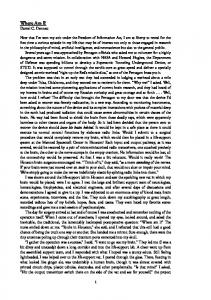
[PDF]Books I am, I am, I am: Seventeen Brushes with ... - Google Sites

I Am, I Am, I Am: Seventeen Brushes With Death - The ... - Google Sites

I Am, I Am, I Am by Maggie O'Farrell book ... - Knopf Doubleday

I am autonomous, you are autonomous - Semantic Scholar

Item 4552 What State Am I? - tlsbooks.com

Where am I and what am I seeing? Algorithms for an autonomous ...