Where Do Return and Volatility Come From? The Case of Asian ETFs
Jose A. Gutierrez Department of Finance, University of Texas at San Antonio
Valeria Martinez Department of Finance, Fairfield University
Yiuman Tse* Department of Finance, University of Texas at San Antonio
December 2007
*Corresponding author. College of Business, 501 West Durango Blvd., San Antonio, Texas 78207. Tel.: 210-458-2503; fax: 210-458-2515; E-mail:
[email protected]
1
Where Do Returns and Volatilities Come From? The Case of Asian ETFs
Abstract We analyze return and volatility of Asian iShares traded in the U.S. The difference in trading schedules between the U.S. and Asia offers a unique market setting that allows us to distinguish various return and volatility sources. We find Asian ETFs have higher overnight volatility than daytime volatility, explained by public information released during each local market’s trading session. Local Asian markets also play an important role in determining each Asian ETF returns. Nonetheless, returns for these funds are highly correlated with U.S. markets, indicative of the investor sentiment effect. Finally, volatility in U.S. markets Grangercauses volatility in all Asian markets analyzed.
JEL Classification: F30; G15 Keywords: International ETF; iShares; returns; variance; diversification
2
Where Do Returns and Volatilities Come From? The Case of Asian ETFs 1. Introduction Where does volatility come from? In previous work volatility is explained by public information, private information, or noise trading1. Because in most markets all three effects take place at the same time, determining which of these three is the source can be a difficult task. There have been various attempts to disentangle these effects by taking advantage of existing market characteristics. For example, Fleming, Kirby, and Ostdiek (2006) analyze volatility for weather sensitive agricultural and energy markets. Under their assumptions, if public information that affects these markets is released at regular intervals throughout the day, then trading and non-trading variances should be equal per unit of time. If there is higher variance during the trading hours then it can be attributed to noise. If trading period variance is normally higher than non-trading period variance, and the difference between these drops during the weather sensitive season, then we can attribute the higher variance to public information. Nonetheless, if the private information flow also rises in the weather sensitive season, then it may be difficult to disentangle these two effects. We extend the work in Fleming et al. (2006), and add value to existing work by analyzing volatility sources for Asian Exchange-Traded Funds (ETFs). The 12-hour difference in schedule between the U.S. and Asian markets enable us isolate the effects of 1
For more information Oldfield and Rogalski (1980), French and Roll (1986), Amihud and Mendelson (1987) Barclay et al. (1990), Stoll and Whaley (1990), Harvey and Huang (1991), Chang et al. (1993), and Chan and Chan (1993).
3
public information, private information, and noise trading. In this setting, more daytime than overnight volatility can be attributed to noise trading or private information, related to trading activity in U.S. markets. More overnight than daytime volatility is attributed to the release of public information in the local Asian market. In addition to volatility, we also analyze Asian ETF returns. Various authors such as Froot and Dabora (1999) find returns are not only determined by the underlying assets they represent but are also influenced by the international market in which they trade. Our results show that Asian ETFs have higher overnight volatility than daytime volatility. We attribute this finding to the release of public information which primarily occurs during each of the local market’s trading session. A closer look at ETF volatilities shows significant bi-directional Granger causality between the U.S. and all Asian markets used in this study. Shifting our focus to returns, we find that Asian markets play an important role in determining Asian ETF returns, however, we also find that returns for these funds are highly correlated with U.S. market returns, indicative of the investor sentiment effect. Taken together, both the U.S. and local Asian markets, contribute to each of the respective funds’ returns, with U.S. markets contributing at least as much and in some cases more to a fund’s return. Overall, the impact of public information in local Asian markets has a significant effect on ETF returns; however the U.S. market investor sentiment effect also plays a determinant role in explaining Asian ETF returns and volatilities.
2. Literature Review There are numerous studies that explain the sources of volatility observed in different markets. Stoll and Whaley (1990) argue that volatility of daytime returns is
4
related to the release of public information during the day. Jones, Kaul, and Lipson (1994), find volatility is higher on days when exchanges are open, even if no trades occur, than when exchanges are closed. French and Roll (1986) posit that the greater trading period variance is due to more private information released during this time period, since traders are more likely to obtain this information and act on it during trading hours. Barclay, Litzenberger, and Warner (1990) attribute the higher weekend volatility on the Tokyo stock exchange to the release of private information. Chan, Fong, Kho, and Stulz (1996) discover that volatility patterns for Asian and European stock are consistent with the arrival of public information, but not private information. Barclay and Hendershott (2003) find that for Nasdaq stocks, the ratio of private to public information during the day is higher than in after hours trading, when there tends to be less informed trades and more liquidity trades. By taking advantage of the natural characteristics of different financial instruments we are able isolate the different volatility sources and better understand the origin of volatility in financial markets. Such is the case of Fleming, Kirby, and Ostdiek (2007), where they analyze volatility for weather sensitive agricultural and energy markets. This market setting allows them to differentiate between the different sources of volatility. While private information and noise trading are more likely during the trading session, public information on these products is evenly distributed throughout the day. They find that there is a strong relationship between prices and public information that cannot be explained by pricing errors or changes in trading activity. Thus volatility in these markets is driven by public information.
5
In the current analysis, we take advantage of the trading schedule differences for international investments, to isolate the local foreign market’s public information from private information and noise trading released during the U.S trading session. However, when it comes to the analysis of foreign investments that trade outside of their home country, there are other factors that come into play. Many of these investments not only reflect public information from their home country, but also display characteristics of the international market in which they trade. This phenomenon is commonly referred to as location of trade or investor sentiment. Evidence of the investor sentiment effect is found in the work of Bodurtha, Kim and Lee (1995), Froot and Dabora (1999), Chan, Hamed, and Lau (2003), and Wang and Jiang (2004). Bodurtha et al. (1995), find that the premiums for the different international closed-end funds tend to move together reflecting the varying sentiment of U.S. investors. Froot et al. (1999) study the trading of the same company stock in different markets. After adjusting for exchange rates, they conclude the same stock trades at different prices in different markets, attributing their results to country specific investor sentiment. Chan et al. (2003) analyze the trading activity of the Hong Kong based company Jardine Group before and after they were de-listed from the Hong Kong Exchange in 1994. After delisting, the core business of the group is maintained in Hong Kong and mainland China, while most of the group’s trading takes place in Singapore. They discover that after delisting the group’s stock from the Hong Kong market, returns are more correlated with the Singapore market and less correlated with the Hong Kong market, consistent with country-specific investor sentiment.
6
Wang and Jiang (2004) analyze Chinese companies that issue A shares in mainland China and H Shares in Hong Kong markets. They find H shares have significant exposure to Hong Kong market factors and behave more like Hong Kong stock than mainland China stock. Choudhry, Lu, and Peng (2006) find significant linkage between the Far East markets before, during, and after the 1997 Asian financial crisis with the U.S. being the most important market. The questions then become more complex than was originally thought. Does volatility come form private information, pubic information, or noise trading?
Are
returns characterized by location of trade or the underlying assets they represent? These are the questions we attempt to answer for the case of Asian ETFs traded in U.S. markets.
3. Data Description Exchange-traded funds (ETFs) are diversified security portfolios that track a stock or bond market index. They can be traded like stock throughout the day using market orders, limit orders, stop orders, margin purchases etc. They trade in both national and regional U.S. exchanges. ETFs have become very popular due to their positive features such as ease of trading, diversification benefits, low expense fees, and potential tax advantage. The latter refers to the fact that in contrast to open-end funds, where the creation or destruction of shares results in a taxable event, ETF investors are not subject to tax consequences as a result of investor demand or liquidations. ETFs create and destroy shares through “in kind transactions or transfers of securities” which are a non-taxable event for the fund. The process is as follows: every day market makers receive information on the demand for (excess of) securities needed to create (destroy) a particular ETF’s shares. They buy
7
(sell) these securities in the capital markets and deposit them (redeem them) with the custodian who issues (destroys) the appropriate number of ETF shares. iShares where created by Barclays in 1996. Since then, the dollar value invested in ETFs has grown to approximately $417 billion, and at the end of 2006, there were nearly 400 different ETF funds. International iShares funds track the Morgan Stanley Capital Indexes which encompass about 85% of each country’s market capitalization. Although the ETFs closely track the index they represent, they do not fully replicate the index. As a result, the ETF and the underlying index will not move in lockstep.2 As reported by Lauricella and Gullapalli (2007), ETF prices are not only determined by fundamental information of the assets they represent, but also by supply and demand in the U.S. market in which they trade. In addition, due to the trading schedule difference between local Asian markets and U.S. markets, prices in each market will not reflect the same amount of information. Since the U.S. market opens and closes at a later time during the day, on any given trading day the U.S. markets can incorporate additional information beyond that released during the Asian trading hours. Rules and regulations for ETFs, may also affect how closely they track the index. For example, the IRS single issue rule points out that an ETF cannot hold a single position that represents more than 25% of their portfolio. Based on this rule, an ETF that tracks any country index that holds a single position of more than 25% of its portfolio will not be able to fully replicate the index. In this study we use daily and intraday data from January 2002 through December 2006 for the following six Asian iShares funds: Hong Kong (EWH), Japan (EWJ), 2
For the sample of funds used in this analysis the correlation between the ETF daytime returns and corresponding local index returns ranges from 27% to 61%.
8
Malaysia (EWM) , Singapore (EWS), South Korea (EWY), Taiwan (EWT), and for the S&P500 (IVV) iShares fund. Daily price data and local market index futures prices come from Commodity Systems Incorporated (CSI). We also use intraday trade data from the Trade and Quote database (TAQ). Initially listed on the AMEX, the iShares used in this analysis migrated to the NYSE in November 2005. Daytime returns are estimated as the log difference between the closing (CLt) and opening (OPt) prices on day t. Overnight returns are the log difference between the opening price on day t (OPt) and the closing price on day t-1 (CLt-1). Daytime returns = log(CLt) - log(OPt)
(1)
Overnight returns = log(OPt) - log(CLt-1)
(2)
Table 1 shows average daily daytime and overnight returns and their standard deviations for each Asian ETF and the U.S. ETF. Consistent with market efficiency, for all the markets, daytime returns and overnight returns are both insignificantly different from zero. For all Asian markets overnight volatility is greater than daytime volatility, and for the U.S. market, daytime volatility is greater than overnight volatility. Daily average dollar volume in shares indicates that the three most active ETFs are Japan (110.1 million), U.S. (76.7 million), and Korea (16.01 million).
4. Main Results We explore the source of Asian ETFs return and variance by analyzing volatility plots, return and volatility correlations, location of trade and public information impact on returns, and Granger causality in returns and volatilities.
9
3.1 Volatility Plots We construct volatility plots for each market using absolute returns of five-minute interval data from January 2002 through December 2006. Figure 1 shows the Taiwan ETF has the highest average intraday volatility (0.089%) and the U.S. ETF the lowest (0.059%) with the rest of the funds ranging in between these values. Each Asian market as well as the S&P 500 presents the typical U-shaped pattern. Admati and Plfeiderer (1988) explain higher volatility at the market opening and close is due to the concentration of informed and uninformed investors. Higher trading volume at these times of the day attracts informed investors who want to use their private information to trade while hiding their identity. Liquidity investors also wish to trade at these times since the competition generated among the various informed investors will tend to reduce trading costs. Brock and Kleidon (1992) explain the U-shape pattern with a different rationale. They claim high trading at the open is caused by the accumulation of overnight information on which investors cannot trade on until the next day’s market opening. Investors also trade heavily around the close in order to re-establish their optimal portfolios. Fama and Roll (1986) argue that the price dynamics around the close tend to be different from the price dynamics associated with normal trading hours.
4.2. Volatility Ratios We construct volatility ratios for each ETF and compare daytime to overnight return volatility using daily data. Table 2 shows that all Asian volatility ratios are lower than one, and range from 0.941 (Malaysia) to 0.517 (Japan). Volatility ratios less than one indicate higher overnight volatility than daytime volatility. The higher overnight
10
volatility signals the release of public information in the local Asian market. These ratios contrast with the U.S. volatility ratio which has a value of 3.53, indicating higher daytime than overnight variance. The higher daytime volatility can be attributed to the release of public information in the U.S. market. To further strengthen these results, we compare daytime and overnight volatilities excluding holidays for each respective Asian market. When Asian holidays are excluded, we expect the observed difference between daytime and overnight volatility to increase which would reduce the values of the observed variance ratios. Table 2 presents the volatility ratios for each market with and without the local holiday effects. The results are in line with our hypothesis. When we exclude local Asian holidays, variance ratios drop across the board in all Asian markets, indicating a greater volatility difference between daytime and overnight returns. These results support the notion that the volatility difference in returns is driven by public information released in each local Asian market. However, the difference between the volatility ratios when Asian holidays are included and excluded is economically insignificant.
4.3 Correlation Analysis Most studies that analyze the relationship between world markets attribute high levels of correlation to location of trade and world market integration. Bodurtha, Kim and Lee (1995), Froot and Dabora (1999), Chan, Hamed, and Lau (2003) determine prices can be influenced by location of trade. Bosner-Neal et al. (1990), Patro (2001), Olienyk, Schwebach and Zumwalt (1999), and Pennathur, Delcoure, and Anderson (2002), find that the more world markets are integrated, the higher the correlation between U.S. and
11
foreign investments , which translates into less diversification benefits from foreign investments. We analyze daily and intraday correlation between the Asian and the U.S. S&P 500 ETF returns and volatilities. As shown in Table 2, Asian funds have at least a 28% daily return correlation and up to 60% with the S&P 500 fund. For the period of our analysis, the Asian fund with the highest daily return correlation with U.S. market is Hong Kong, followed by Japan, Taiwan, Korea, Singapore, and Malaysia, with correlation coefficients of 0.603, 0.571, 0.564, 0.545, 0.466, and 0.282 respectively. In terms of daily volatility, the highest correlation with the U.S. is found in Hong Kong (0.427), Korea (0.381), and Taiwan (0.378), and the Asian market with the lowest volatility correlation with the U.S. is Malaysia (0.128). The high correlation values suggest that Asian ETFs have limited diversification benefits. In addition, the strong relationship between these funds and the U.S. equity market shows that location of trade, as well as world market integration are both important factors in determining each of the ETFs’ returns. Next we obtain the U.S. dollar-denominated ETF returns, as well as transformed ETF returns (transformed using the dollar / local Asian market exchange rate) and study the correlation between the Asian ETF returns, the transformed ETF returns, and the leading local Asian market index returns. As evidenced by Table 3, the correlation between the Asian ETF return and the transformed ETF return ranges from 0.996 (Hong Kong) to 0.754 (Malaysia). In the case of Hong Kong, this high foreign exchange effect is a function of the Hong Kong dollar being pegged to the U.S. dollar.
12
In Table 3 we also present the correlation between the Asian ETF returns and the returns from the leading local Asian market index. These correlations range from 0.692 (South Korea) to 0.539 (Hong Kong). Although these values are high, it is apparent that the Asian ETFs are not designed to fully replicate the underlying index that they represent, but rather provide returns that generally correspond to the yield performance of the underlying index. Further evidence of this can be found in Appendix 1, which provides a breakdown of the top 10 holdings for both the ETF and the leading local Asian market index as of December 2006.
4.4 Location of Trade and Market Integration To further study the source of Asian iShares returns we use a simple regression analysis of contemporaneous variables. We regress each Asian ETF’s daytime returns on the S&P 500 iShares daytime returns and the local market’s overnight returns, represented by the local index’s nearest futures contract. Arett=b0+b1USrett+b2Indexrett+b3Ahdumt+et
(3)
Where: Arett= daytime return of each Asian iShares; USrett= daytime return of the S&P 500 iShares; Indexrett= overnight return in each Asian market’s most representative market index futures contract; Ahdumt= dummy variable equal to one when there is a holiday in that particular Asian market and zero otherwise; and et = error term.
13
Table 4 shows that for Hong Kong, Japan, Korea, and Taiwan, the U.S. market returns explain a greater portion of Asian ETF returns than do the returns from the local market, as measured by the b1 and b2 coefficients, respectively. For example, in the case of Hong Kong, the b1 coefficient (t-statistic) is 0.477 (8.66) whereas the b2 coefficient is 0.284 (4.46). In the case of Malaysia and Singapore, however, the above does not hold. For Malaysia, the local market explains more of the ETF returns, while for Singapore the local market and the U.S. market explain approximately equal portions of the Singapore ETF returns. The significant contribution of U.S. market returns to international investment returns is consistent with the importance of location of trade and world market integration in explaining foreign investment returns. In addition, the important contribution of each local market’s returns to each Asian ETF, confirms public information released in each local market also plays an important role in explaining these ETFs’ returns. It is important to point out that these results are qualitatively the same after controlling for the foreign exchange rate between the U.S. and the local Asian market. Furthermore, holidays do not have a significant effect on returns for any Asian country.
4.5 Granger Causality in Returns and Volatilities We analyze the lead-lag relationship in returns and volatilities between the U.S. market and each Asian market using 5-minute-interval intraday data. The equations used in the analysis are as follows. For returns: Arett= α10 + B11(L)Arett-1 +B12(L) USrett-1+e1t USrett= α20 + B21(L)Arett-1 +B22(L)USrett-1+e2t
(4)
14
Where : Arett= daytime return of each Asian iShares; USrett= daytime return of the S&P iShares; αi0= vector of constants; Bij = lagged values of Aret and USret; and eit= error terms.
For volatilities: |Arett|= α10 + B11(L)|Arett-1| +B12(L)|USrett-1|+e1t
|Usrett|= α20 + B21(L)|Arett-1| +B22(L)|USrett-1|+e2t
(5)
Where : |Arett|= absolute value of daytime return of each Asian iShares; |USrett|= absolute value of daytime return of the S&P iShares; αi0= vector of constants; Bij = lagged values of |Aret| and |USret|; and eit= error terms. Based on AIC and SBC criteria, as well as error autocorrelation for each system of equations, we use 8 lags to analyze Granger causality in returns and 24 lags for volatility. Panel A of Table 5 shows Chi-squared tests for Granger causality in returns between each Asian market and the U.S. We observe U.S. ETF returns Granger-cause returns for all Asian markets at a significance level of 0.1%. In contrast, only Japan and
15
Taiwan Granger-cause U.S. returns at significance levels of 0.5% and 0.1% respectively. These results are consistent with those observed in Table 4, highlighting the importance of the U.S. market, in which these ETFs trade.3 Panel B of Table 5 shows Granger causality in volatility. With the exception of Malaysia, we observe significant bi-directional Granger causality between the U.S. and all Asian markets. These results are consistent with the efficient transmission of information across world markets.
5. Summary of Findings By taking advantage of the trading schedule difference between the U.S. and Asian markets, we are able to distinguish between different return and volatility sources for Asian iShares. We find that Asian ETF returns are explained by both U.S. returns (location of trade) and local Asian market returns. The location of trade or investor sentiment effect is further supported by the high return correlation between the Asian and U.S. ETFs. In the case of volatility, we observe higher overnight than daytime volatility, credited to the release of public information in each local market. Finally, Granger causality analysis of returns and volatilities shows the U.S. Granger-causes returns in all Asian markets. In addition, we find bi-directional Granger causality in volatilities, between the U.S. and the six Asian markets analyzed. These results are consistent with the absence of arbitrage and confirm the existence of market efficiency.
3
Dummies for Mondays and holidays (not reported) are insignificant.
16
Overall, local market information and returns play an important role in explaining Asian ETF returns and volatilities. Nonetheless, returns and volatilities are heavily influenced by the U.S. market in which they trade in.
17
References Barclay, M. J., Litzenberger R.H., & Warner, J. B. (1990). Private information, trading volume and stock return variances. Review of Financial Studies 3, 233-253. Barclay, M. J., & Hendershott, T. (2003). Price discovery and trading after hours. Review of Financial Studies 16, 1041-1073. Baxter, M., & Jermann, U. J. (1997). The international diversification puzzle is worse than you think. The American Economic Review 87, 170-180. Bodurtha, J.N., Kim, D.S., & Lee, C.M.C. (1995). Closed-end country funds and U.S. market sentiment. Review of Financial Studies 8, 879-918. Bonser-Neal, C. Brauer, G., Neal, R., & Wheatley, S. (1990). International investment restrictions and closed-end country fund prices. Journal of Finance 45, 523-547. Chan, K., & Chan, Y.C. (1993). Price volatility in the Hong Kong stock market: a test of the information and trading noise hypothesis. Pacific-Basin Financial Journal 1, 189-202. Chan, K., Fong, W. M., Kho, B. C., & Stulz, R. M. (1996). Information trading and stock returns: Lessons from dually-listed securities. Journal of Banking and Finance 20, 1161-1187. Chan, K., Hamed, A., & Lau, S. T. (2003). What if trading location is different from business location? Evidence from the Jardine Group. Journal of Finance 58, 1221-1246. Chang, R.P., Fukuda, T., Rhee, S.G., & Takano, M. (1993). Interday and intraday return behavior of the TOPIX. Pacific-Basin Financial Journal 1, 67-95. Choudry, T., Lu, L., & Peng, K. (2006). Common stochastic trends among Far East stock prices: Effects of the Asian financial crisis. International Review of Financial Analysis 16, 242-261.
18
French, K. R., & Poterba, J. M. (1991). Investor diversification and international equity markets. The American Economic Review 81, 222-226. French, K.R., & Roll, R. (1986). Stock return variances: the arrival of information and the reaction of traders. Journal of Financial Economics 17, 5-26. Fleming, J., Kirby, C., & Ostdiek, B. (2006). Information, trading and volatility: Evidence from weather-sensitive markets. Journal of Finance 61, 2899-2930. Froot, K.A., & Dabora, E.M. (1999). How are stock prices affected by the location of trade? Journal of Financial Economics 53, 189-216. Jones, C.M., Kaul, & G. Lipson, M. (1994). Information trading and volatility. Journal of Financial Economics 36, 127-154. Kang, J. K., & Stulz, R. M. (1997). Why is there a home bias? An analysis of foreign portfolio equity ownership in Japan. Journal of Financial Economics 46, 3-28 Lauricella, T., & Gullapalli, D. (2007), Fast Money Crowds Embrace ETFs, adding risk for individual investors. The Wall Street Journal. Oldfield, S., & Rogalski, R. (1980). A theory of common stock returns over trading and nontrading periods. Journal of Finance 35, 729-751. Olienyk, J.P., Schwebach, R.G., & Zumwalt, J. K. (1999). WEBS, SPDRs, and country funds: an analysis of international cointegration. Journal of Multinational Financial Management 9, 217–232. Patro, D.K. (2001). Market segmentation and international asset prices: evidence from the listing of world equity benchmark shares. Journal of Financial Research 24, 83-98. Pennathur, A.K. Delcoure, N., & Anderson, D. (2002). Diversification benefits of iShares and closed-end funds. Journal of Financial Research 25, 541-557.
19
Stoll, H., & Whaley R. (1990). Stock Market Structure and Volatility. Review of Financial Studies 3, 37-71. Tesar, L., & Werner, I. (1995). Home bias and high turnover. Journal of International Money and Finance 14, 467-492. Wang, S. S., & Jiang, L. (2004). Location of trade, ownership restrictions, and market illiquidity: Examining Chinese A- and H- shares. Journal of Banking and Finance 28, 1273-1297.
20
15:30
15:00
14:30
14:00
13:30
13:00
12:30
12:00
11:30
11:00
10:30
10:00
9:30
Avg. Abs. Returns
EST
Korea
0.2
0.1
EST 0.15 0.2
0.1
0 0
12:30
12:00
11:30
11:00
10:30
15:00 15:30
15:00 15:30
15:00 15:30
14:30
Taiwan
14:30
0.25
14:00
EST
14:30
0
13:30
0.1
14:00
0.05
13:30
0.2
14:00
0.15
13:30
Singapore
13:00
0.25
13:00
EST
13:00
0.05 0.05
12:30
Japan
12:00
EST
12:30
0.25 11:30
0 10:00
Hong Kong
12:00
0.1
11:30
0.05
11:00
0.25
10:30
0
11:00
0 9:30
0.05 0.05
10:30
0.2
9:30
0.1 Avg. Abs. Returns
0.2
10:00
0.15
Avg. Abs. Returns
15:30
15:00
14:30
14:00
13:30
13:00
12:30
12:00
11:30
11:00
10:30
10:00
9:30
Avg. Abs. Returns 0.15
10:00
0.15
Avg. Abs. Returns
15:30
15:00
14:30
14:00
13:30
13:00
12:30
12:00
11:30
11:00
10:30
10:00
9:30
Avg. Abs. Returns 0.25
9:30
15:30
15:00
14:30
14:00
13:30
13:00
12:30
12:00
11:30
11:00
10:30
10:00
9:30
Avg. Abs. Returns
Figure 1 Intraday Volatility Plots
Volatility plots for average absolute returns obtained from five-minute intervals from January 2002 to December 2006 for each Asian ETF and the S&P500 ETF. 0.25
Malaysia
0.15
0.2
0.1
EST
0.25
U.S.
0.15 0.2
0.05 0.1
0
EST
21
Table 1 Descriptive Statistics Daytime returns are estimated as the difference between the U.S. market’s closing and opening price for each ETF. Daytime returns = log(CLt) - log(OPt). Overnight returns are estimated as the difference between the U.S. market’s opening price and the previous day’s closing price for each ETF. Overnight returns = log(OPt) - log(CLt-1). Daily volume, returns, and standard deviation of returns are obtained using data from January 2002 to December 2006.
Average Returns
Std. Dev of Returns
Daytime
Overnight
Daytime
Overnight
Volume ($m)
Hong Kong
(EWH)
-0.0005
0.0010
0.0112
0.0127
7.87
Japan
(EWJ)
0.0004
0.0001
0.0081
0.0112
110.12
Korea
(EWY)
-0.0012
0.0020
0.0133
0.0174
16.01
Malaysia
(EWM)
-0.0001
0.0005
0.0091
0.0094
3.10
Singapore
(EWS)
-0.0003
0.0009
0.0121
0.0126
2.95
Taiwan
(EWT)
-0.0018
0.0020
0.0147
0.0172
13.77
(IVV)
0.0000
0.0002
0.0092
0.0049
76.72
U.S.
22
Table 2 Variance Ratios and Correlations The table shows variance ratios estimated as the ratio of daytime return variance divided by overnight return variance. VR1 is the variance ratio of daytime to overnight return variance of each Asian and U.S. iShares. VR2 is the variance ratio of daytime to overnight return variance of each iShares excluding holidays in each respective Asian market. Daily return and volatility correlations are estimated using daily close to close price returns. Daily return and volatility correlations are estimated using the log difference between the U.S. market’s closing price and the previous day’s closing price. ∆CLt = log(CLt) – log(CLt-1).Intraday return and volatility correlations are estimated using 5-minute intraday interval returns.
Variance Ratios VR1
VR2
Correlations Daily Intraday Return Volatility Return Volatility
Hong Kong
(EWH)
0.776
0.757
0.603
0.427
0.119
0.110
Japan
(EWJ)
0.517
0.507
0.571
0.325
0.434
0.299
Korea
(EWY)
0.589
0.574
0.545
0.381
0.170
0.143
Malaysia
(EWM)
0.941
0.932
0.282
0.128
0.068
0.075
Singapore
(EWS)
0.922
0.912
0.466
0.358
0.105
0.092
Taiwan
(EWT)
0.734
0.702
0.564
0.378
0.158
0.121
(IVV)
3.531
U.S.
23
Table 3 ETF Return, Transformed ETF Return and Asian Index Return Correlations The table shows the correlation between the ETF return, the ETF return transformed by the U.S. and local Asian market exchange rate, and the return of the leading local Asian market index.
Hong Kong (EWH)
Singapore (EWS)
Taiwan (EWT)
Japan (EWJ)
Korea (EWY)
Malaysia (EWM)
Asian ETF Return
Trans Asian ETF Ret
Asian Index Return
Asian ETF Ret Trans Asian ETF Ret Asian Index Return
1.00000 0.99691 0.53904
1.00000 0.53946
1.00000
Asian ETF Ret Trans Asian ETF Ret Asian Index Return
1.00000 0.96342 0.57135
1.00000 0.55831
1.00000
Asian ETF Ret Trans Asian ETF Ret Asian Index Return
1.00000 0.95451 0.64203
1.00000 0.61316
1.00000
Asian ETF Ret Trans Asian ETF Ret Asian Index Return
1.00000 0.90943 0.58759
1.00000 0.54934
1.00000
Asian ETF Ret Trans Asian ETF Ret Asian Index Return
1.00000 0.88496 0.69202
1.00000 0.61820
1.00000
Asian ETF Ret Trans Asian ETF Ret Asian Index Return
1.00000 0.75432 0.54179
1.00000 0.43013
1.00000
24
Table 4 Location of Trade vs. Release of Public Information The table shows the results for the regression: Arett= b0 + b1USrett + b2Indexrett+ b3Fxret+ b4Ahdum +et,. Where Arett is the daytime return of each Asian iShares; USrett is the daytime return of the S&P500 iShares; Indexrett is the overnight return in each Asian market’s most representative market index futures contract; Ahdum is a dummy variable equal to one when there is a holiday in that particular Asian market and zero otherwise; and et, is the error term. T-statistics are presented in parenthesis below the coefficients. Regression errors are corrected for hetersoskedasticity using White (1980). Arett= b0+b1USrett+b2Indexrett+b3Ahdum + et Dependent Variable Hong Kong Japan Korea Malaysia Singapore (EWH) (EWJ) (EWY) (EWM) (EWS)
Taiwan (EWT)
b0
-0.001 (-1.68)
0.000 (1.41)
-0.001 (-3.78)
0.000 (-0.80)
-0.001 (-1.71)
-0.002 (-5.36)
b1
0.480** (8.67)
0.432** (15.15)
0.505** (9.15)
0.158** (3.74)
0.313** (4.85)
0.731** (8.18)
b2
0.283** (4.45)
0.304** (9.86)
0.310** (6.54)
0.343** (4.05)
0.386** (5.26)
0.237 (1.90)
b3
0.008* (2.46)
0.000 (-0.42)
0.000 (0.84)
0.000 (-1.77)
0.002 (-1.37)
0.001 (0.95)
0.29
0.51
0.35
0.08
0.20
0.31
2
R Adj.
* Significant at the 5% level ** Significant at the 1% level
25
Table 5 Granger Causality Between U.S. and Asian Markets The table shows Wald coefficient tests for Granger causality from the U.S. ETF to each Asian ETF and vice versa, from January 2002 through December 2006. Panel A shows causality in returns and Panel B shows causality in volatilities. Chi-squared p-values are presented in parentheses below the coefficients. Pvalue coefficients for 5 and 35 lag Q-statistics on residual autocorrelation are presented at the foot of each panel. Results are generated using two-equation VAR systems with eight lags for return models and 24 lags for volatility models. Panel A: Causality in Returns Arett= α10 + B11(L)Arett-1 +B12(L) USrett-1+e1t USrett= α20 + B21(L)Arett-1 +B22(L)USrett-1+e2t
U.S. Granger-causes Asia
(1)
(2)
(3)
(4)
(5)
(6)
Hong Kong
Japan
Korea
Malaysia
Singapore
Taiwan
1894.3** (0.000)
1861.0** (0.000)
511.2** (0.000)
978.3** (0.000)
1504.0** (0.000)
1495.5** (0.000)
p-value Q(5) p-value Q(35)
0.73 0.05
0.99 0.99
0.94 0.60
0.65 0.80
0.92 1.00
0.95 0.97
Asia Granger-causes U.S.
6.57 (0.584)
64.54** (0.000)
11.96 (0.153)
6.08 (0.639)
3.93 (0.864)
23.68* (0.003)
p-value Q(5) p-value Q(35)
0.61 0.99
0.28 0.10
1.00 0.93
0.75 1.00
0.82 0.70
0.99 0.94
Panel B: Causality in Volatility |Arett|= α10 + B11(L)|Arett-1| +B12(L)|USrett-1|+e1t |Usrett|= α20 + B21(L)|Arett-1| +B22(L)|USrett-1|+e2t (1)
(2)
(3)
(4)
(5)
(6)
Hong Kong
Japan
Korea
Malaysia
Singapore
Taiwan
U.S. Granger-causes Asia
121.7** (0.000)
192.3** (0.000)
84.6** (0.000)
36.6 (0.048)
59.6* (0.000)
160.7** (0.000)
p-value Q(5) p-value Q(35)
0.99 1.00
0.99 1.00
1.00 1.00
1.00 1.00
0.99 1.00
0.86 1.00
Asia Granger-causes U.S.
68.78** (0.000)
60.82** (0.000)
163.59** (0.000)
36.90 (0.045)
58.41* (0.000)
48.77* (0.002)
p-value Q(5) p-value Q(35)
1.00 1.00
0.87 1.00
0.94 0.99
0.97 1.00
0.98 1.00
0.94 0.99
n = 79,455
* Significant at the 0.5% level
** Significant at the 0.1% level
26
Appendix The table shows the top 10 holdings (in percentage) of both the ETF and the leading local Asian market index as of December 2006. ETF Hong Kong (EWH) Hutchison Whampoa Ltd Cheung Kong Holdings Ltd Sun Hung Kai Properties Ltd Hong Kong Exchanges and Clearing Ltd Espirit Holdings Ltd Hang Seng Bank Ltd Swire Pacific Ltd 'A' CLP Holdings Ltd BOC Hong Kong Holdings Ltd LI & Fung Ltd
Japan (EWJ) Toyota Motor Corp Mitsubishi UFJ Financial Gro Mizuho Financial Group Inc Canon Inc Sumitomo Mitsui Financial Group Honda Motor Co Ltd Takeda Pharmaceutical Co Ltd Sony Corp Nippon Steel Corp Matsushita Electric Indust
Taiwan (EWT) Taiwan Semiconductor Manufac HON HAI Precision Industry Co Ltd Cathay Financial Holding Co Ltd MediaTek Inc Nan Ya Plastics Corp United Microelectronics Corp AU Optronics Corp Formosa Plastics Corp China Steel Corp Chunghwa Telecom Co Ltd
Index
8.68% 8.10% 6.78% 6.27% 5.46% 4.28% 3.82% 3.67% 3.65% 3.30% 54.01%
5.80% 3.03% 2.22% 2.08% 2.04% 1.92% 1.85% 1.76% 1.37% 1.36% 23.43%
12.23% 9.75% 3.59% 3.42% 2.97% 2.84% 2.83% 2.78% 2.75% 2.45% 45.61%
Hang Seng China Mobile Ltd HSBC Holdings PLC China Life Insurance Co Ltd Hong Kong Exchanges and Clearing Ltd China Construction Bank Corp Industrial & Commercial Bank of China Cheung Kong Holdings Ltd CNOOC Ltd Sun Hung Kai Properties Ltd Hutchison Whampoa Ltd
Nikkei 225 Fanuc Ltd Kyocera Corp TDK Corp Canon Inc KDDI Corp Takeda Pharmaceutical Co Ltd Shin-Etsu Chemical Co Ltd Honda Motor Co Ltd Tokyo Electron Ltd Softbank Corp
TAIEX TSMC HON HAI Precision Industry Co Ltd Formosa Petrochemical Corp Cathay Financial Holding Co Ltd Nan Ya Plastics Corp Chunghwa Telecom Co Ltd MediaTek Inc China Steel Corp Formosa Plastics Corp Formosa Chemicals & Fibre Corp
14.23% 13.94% 6.73% 4.88% 4.53% 4.31% 3.51% 3.34% 3.27% 3.24% 61.99%
2.94% 2.55% 2.42% 2.32% 2.12% 1.98% 1.97% 1.92% 1.84% 1.70% 21.74%
7.24% 6.74% 4.09% 3.32% 3.03% 2.78% 2.59% 2.47% 2.37% 2.11% 36.75%
27
Korea (EWY) Samsung Electronics Co Ltd POSCO Kookmin Bank Shinhan Financial Group Co Ltd Hyundai Heavy Industries SK Telecom Co Ltd Hyundai Motor Co Korea Electric Power Corp Shinsegae Co Ltd Samsung Heavy Industries
Singapore (EWS) Singapore Telecommunications Ltd United Overseas Bank Ltd DBS Group Holdings Ltd Oversea-Chinese Banking Corp Keppel Corp Ltd CapitaLand Ltd Singapore Airlines Ltd City Developments Ltd Singapore Exchange Ltd Singapore Press Holdings Ltd
Malaysia (EWM) Bumiputra-Commerce Holdings Bhd Malayan Banking Bhd IOI Corp Bhd Genting Bhd Tenaga Nasional Bhd Sime Darby Bhd MISC Bhd Telekom Malaysia Bhd Public Bank BHD Resorts World BHD
14.69% 7.83% 6.49% 4.19% 3.73% 2.96% 2.66% 2.51% 2.02% 1.91% 48.99%
11.74% 11.60% 11.09% 10.09% 5.39% 4.94% 4.51% 4.15% 3.29% 3.11% 69.91%
10.29% 8.42% 6.48% 5.52% 5.35% 5.23% 4.03% 3.82% 3.79% 3.14% 56.07%
KOSPI Samsung Electronics Co Ltd POSCO Hyundai Heavy Industries Kookmin Bank Shinhan Financial Group Co Ltd Korea Electric Power Corp SK Telecom Co Ltd Hyundai Motor Co LG Corp Shinsegae Co Ltd
STI Singapore Telecommunications Ltd United Overseas Bank Ltd DBS Group Holdings Ltd Oversea-Chinese Banking Corp Singapore Exchange Ltd Keppel Corp Ltd CapitaLand Ltd Singapore Airlines Ltd Hongkong Land Holdings Ltd Jardine Matheson Holdings Ltd
KLSE Malayan Banking Bhd Tenaga Nasional Bhd Bumiputra-Commerce Holdings Bhd MISC Bhd Telekom Malaysia Bhd IOI Corp Bhd Public Bank BHD Genting Bhd Sime Darby Bhd Petronas Gas BHD
10.13% 8.02% 4.33% 3.89% 3.34% 2.82% 2.29% 1.82% 1.67% 1.59% 39.89%
10.98% 10.31% 8.99% 8.19% 6.30% 6.23% 4.86% 4.02% 3.20% 3.02% 66.09%
6.21% 5.64% 5.33% 5.02% 4.97% 4.95% 4.89% 4.03% 3.85% 2.99% 47.87%
28