15 FEBRUARY 2003
619
BRUNKE ET AL.
Which Bulk Aerodynamic Algorithms are Least Problematic in Computing Ocean Surface Turbulent Fluxes? MICHAEL A. BRUNKE Institute of Atmospheric Physics, The University of Arizona, Tucson, Arizona
CHRIS W. FAIRALL National Oceanic and Atmospheric Administration/Environmental Technology Laboratory, Boulder, Colorado
XUBIN ZENG Institute of Atmospheric Physics, The University of Arizona, Tucson, Arizona
LAURENCE EYMARD Centre d’Etude des Environments Terrestre et Plane´ taires, Velizy, France
JUDITH A. CURRY Department of Earth and Atmospheric Sciences, Georgia Institute of Technology, Atlanta, Georgia (Manuscript received 14 November 2001, in final form 5 July 2002) ABSTRACT Bulk aerodynamic algorithms are needed to compute ocean surface turbulent fluxes in weather forecasting and climate models and in the development of global surface flux datasets. Twelve such algorithms are evaluated and ranked using direct turbulent flux measurements determined from covariance and inertial-dissipation methods from 12 ship cruises over the tropical and midlatitude oceans (from about 58S to 608N). The four least problematic of these 12 algorithms based upon the overall ranking for this data include the Coupled Ocean–Atmosphere Response Experiment (COARE) version 3.0 and The University of Arizona (UA) schemes as well as those used at the European Centre for Medium-Range Weather Forecasts (ECMWF) and the National Aeronautics and Space Administration (NASA) Data Assimilation Office for version 1 of the Goddard Earth Observing System reanalysis (GEOS-1). Furthermore, the four most problematic of these algorithms are also identified along with possible explanations. The overall ranking is not substantially affected by the use of the average of covariance and inertialdissipation flux measurements or by taking into consideration measurement uncertainties. The differences between computed and observed fluxes are further evaluated as a function of near-surface wind speed and sea surface temperature to understand the rankings. Finally, several unresolved issues in terms of measurement and algorithm uncertainties are raised.
1. Introduction Knowledge of the sea surface turbulent fluxes; that is, latent and sensible heat fluxes as well as momentum flux or wind stress, is important for understanding air– sea interactions, forcing ocean models, evaluating numerical weather prediction and coupled atmosphere– ocean models, understanding the ocean heat and freshwater budget, and the partitioning of the global poleto-equator transport between the atmosphere and ocean. Corresponding author address: Michael A. Brunke, Department of Atmospheric Sciences, The University of Arizona, Physics–Atmospheric Sciences Bldg., P.O. Box 210081, Tucson, AZ 85721. E-mail:
[email protected]
q 2003 American Meteorological Society
The ocean surface turbulent fluxes are calculated directly from the covariances of wind speed, humidity, and temperature with vertical velocities such that
t 5 r a [(w9u9 ) 1 (w9y 9 ) 2 ]1/2 , LH 5 r a Ly w9q9, SH 5 r a C p w9u9,
and
(1) (2) (3)
where t, LH, and SH are the wind stress, latent heat flux, and sensible heat flux, respectively; r a is the density of air; L y is the latent heat of vaporization; C p is the specific heat of air at constant pressure; and w9F9 (with F 5 u, y , q, or u) is the covariance between the
620
JOURNAL OF CLIMATE
turbulent perturbations of vertical velocity and F.1 These covariances can be directly computed using highfrequency measurements of turbulent perturbations. Direct measurements of turbulent fluxes are made only during field experiments. Hence, for modeling and dataset generation purposes, it is desirable to use bulk aerodynamic algorithms that relate the turbulent fluxes to bulk meteorological variables (e.g., surface temperature, surface air temperature, humidity, and wind). These bulk algorithms use Monin–Obukhov similarity theory in which three turbulent parameters are defined: u* 5 [(w9u9 ) 2 1 (w9y 9 ) 2 ]1/4 , q* 5 2
w9q9 , u*
and
(4) (5)
w9u9 , (6) u* where u* is the scaling parameter for wind or friction velocity, q* is the scaling parameter for humidity, and u* is the scaling parameter for potential temperature. Thus, 2 t 5 r a u*, (7)
u* 5 2
LH 5 2r a Ly u*q*,
and
(8)
SH 5 2r a C p u*u*. (9) The turbulent fluxes are directly related to the mean meteorological measurements by defining turbulent exchange coefficients, u*2 CD 5 , (10) SU CE 5 2
u*q* , S(q s 2 q a )
and
(11)
u*u* , (12) S(u s 2 u a ) where C D , C E , and C H are the exchange coefficients for momentum, moisture, and heat respectively; U is the near-surface wind speed; S is the near-surface wind speed with the inclusion of convective gustiness if it is considered (see the appendix; S 5 U otherwise); q s and q a are the surface and near-surface atmospheric specific humidities, respectively; and u s and u a are the surface and near-surface air potential temperatures, respectively. Thus, t 5 r a C D SU, (13) CH 5 2
LH 5 r a Ly C E S(q s 2 q a ), SH 5 r a C p C H S(u s 2 u a ).
and
(14) (15)
1 Here, u is the zonal wind speed, y is the meridional wind speed, w is the vertical wind speed, q is specific humidity, and u is potential temperature.
VOLUME 16
Bulk algorithms differ in how they parameterize these exchange coefficients. The algorithms also differ in how the wave spectrum is considered, which in turn affects the parameterization of the roughness length for momentum. Most algorithms explicitly consider only gravity waves; a few recently developed algorithms, the Bourassa–Vincent–Wood (BVW; Bourassa et al. 1999) and Clayson–Fairall–Curry (CFC; Clayson et al. 1996) algorithms, also include the effects of capillary waves. Other differences among algorithms include those in the parameterization of the roughness lengths for heat and moisture, whether or not the effect of the salinity of seawater is considered in the calculation of surface saturated humidity, and whether or not convective gustiness is considered at low wind speeds. These differences have been extensively discussed in Zeng et al. (1998) and Brunke et al. (2002). All of these factors contribute to the differences between the fluxes calculated by the algorithms that have been shown to be particularly important in modeling (e.g., Webster and Lukas 1992; Miller et al. 1992; Wang et al. 1996). In addition to their use in weather and climate models, algorithms are also used to generate datasets of turbulent sea surface fluxes. Recently, several groups have developed global datasets of these fluxes derived from satellite observations such as the Hamburg Ocean–Atmosphere Parameters from Satellite Data (HOAPS; see online at http://www.hoaps.zmaw.de), the Goddard SatelliteBased Surface Turbulent Fluxes (GSSTF; Chou et al. 2001, 2002; see online at http://daac.gsfc.nasa.gov/ CAMPAIGNpDOCS/hydrology/hdpmain.shtml), and the Japanese Ocean Flux Data Sets with Use of Remote Sensing Observations (J-OFURO; Kubota et al. 2002; see online at http://dtsv.scc.u-tokai.ac.jp). Brunke et al. (2002) showed that while the flux differences from various datasets such as these are primarily caused by differences in the bulk variables, algorithm differences still play a significant role. In this paper, the performance of 12 bulk aerodynamic algorithms used in weather and climate models as well as satellite dataset development is evaluated based on extensive inertial-dissipation and covariance flux measurements taken from ships during 12 experiments in the Tropics and midlatitudes. Previously, such comparisons have been conducted using data from one or two such experiments (Brunke et al. 2002; Zeng et al. 1998; Chang and Grossman 1999), resulting in a limited evaluation of the algorithms and interpretation of the algorithm uncertainties. Of these 12 algorithms, we choose what we believe based on the data used herein to be the ‘‘best’’ or least problematic. In interpreting our selection, the reader is cautioned that alternative selection criteria could result in alternative recommendations. The algorithms included in this study are explained in the appendix, and the data from the 12 ship cruises are described in section 2. Results are presented in section 3 and further discussed in section 4.
15 FEBRUARY 2003
621
BRUNKE ET AL. TABLE 1. The cruises for which data is used in this study.
Experiment
Acronym
Atlantic Stratocumulus Transition Experiment Couplage avec l’Atmosphe`re en Conditions Hivernales Coupled Ocean–Atmosphere Response Experiment Fronts and Atlantic Storm Track Experiment Flux, E´tat de la Mer et Te´le´de´tection en Condition de Fetch Variable Joint Air–Sea Monsoon Experiment Kwajalein Experiment Mooringsa Nauru ’99 Pan-American Climate Study Flux 1999b San Clemente Ocean Probing Experiment Tropical Instability Wave Experiment
Institution
Ship or platform
Time period
Reference
ASTEX
ETL
R/V Malcolm Baldridge
Jun 1992
White et al. (1995)
CATCH
CETP
R/V Le Suroıˆt
Jan–Feb 1997
Eymard et al. (1999)
COARE
ETL
R/V Moana Wave
Nov 1991–Feb 1992
Young et al. (1992)
FASTEX
ETL
R/V Knorr
Dec 1996–Jan 1997
Hare et al. (1999)
FETCH JASMINE KWAJEX
CETP ETL ETL ETL ETL
R/V R/V R/V R/V R/V
L’Atalante Ronald H. Brown Ronald H. Brown Ronald H. Brown Ronald H. Brown
Mar–Apr. 1998 May 1999 Jul–Sep 1999 Sep–Oct 1999 Jun–Jul 1999
Hauser et al. (2002) Fairall et al. (2000a)
PACSF99
ETL
R/V Ronald H. Brown
Nov–Dec 1999
SCOPE TIWE
ETL ETL
R/P FLIPc R/V Moana Wave
Sep 1993 Nov–Dec 1991
Fairall et al. (2000b)
Fairall and Edson (1994) Chertock et al. (1993)
A cruise to service buoys in the North Pacific. Part of the Eastern Pacific Investigation of Climate Processes in the Coupled Ocean–Atmosphere System (EPIC). c Scripps Institution of Oceanography’s Floating Instrument Platform. a
b
2. Data The observational data come from two sources. Ten datasets are from experiments operated by the National Oceanic and Atmospheric Administration (NOAA) Environmental Technology Laboratory (ETL; Table 1; data available from ETL). The other two sets are from the Centre d’Etude des Environments Terrestre et Plane´taires [CETP; Table 1; data available from CETP at the AUTOFLUX Linked Base for Automatic Transfer at the Ocean Surface (ALBATROS) Web site: http:// dataserv.cetp.ipsl.fr; Weill et al. 2003]. Figure 1 shows the locations of these 12 cruises. Table 1 presents the time period in which measurements were taken, and Table 2 shows the heights of the instrumentation used to obtain mean measurements for wind speed and di-
rection, temperature, and humidity as well as the depth at which bulk sea surface temperature (SST) was measured during each cruise. During the ETL cruises, the mean air temperature and humidity were measured using a Vaisala sensor (an HMP-35 in the early 1990s and an HMP-235 for the later cruises) and improved meteorological (IMET) sensors. The IMET measurements were preferred for the Fronts and Atlantic Storm Track Experiment (FASTEX) and the Vaisala measurements were preferred for the other ETL cruises. Mean wind speed was measured using a Gill sonic anemometer (INUSA RS-2 or RS-2A). Bulk SST was measured by a floating thermistor at a depth of about 0.05 m (Table 2). Turbulent measurements of wind and temperature were made by the sonic anemometer, and turbulent mea-
FIG. 1. The ship trajectories of each of the 12 cruises used in this comparison.
622
JOURNAL OF CLIMATE
TABLE 2. The height of the instruments used to obtain mean wind speed, air temperature, and air humidity. Instrumentation height or depth (m) Experiment ASTEX CATCH COARE FASTEX FETCH JASMINE KWAJEX Moorings Nauru ’99 PACSF99 SCOPE TIWE
Sonic Air anemometer temperature 21.00 17.40 15.00 19.20 17.80 17.70 17.70 17.70 17.70 17.70 11.00 15.00
20.00 16.40 14.00 17.50 17.55 14.80 14.80 14.80 14.80 14.80 11.00 14.00
Air humidity
Sea surface temperature
20.00 16.40 14.00 17.50 17.55 14.80 14.80 14.80 14.80 14.80 11.00 14.00
0.05 2.50 0.05 0.05 2.50 0.05 0.05 0.05 0.05 0.05 0.05 0.05
surements of humidity were made by a high-speed infrared hygrometer (Ophir Corporation IR-2000). For the CETP cruises, mean air temperature and humidity was measured by a Vaisala HMP-35D and HMP-233, respectively. A Gill Solent sonic symmetric anemometer was also used along with two Young propeller-vane anemometers (each located 1 m horizontally from the sonic anemometer). The sonic anemometer measurements are used herein. Bulk SST was measured using a SBE 21 SEACAT thermosalinograph at a depth of 2.5–3 m (Table 2). The sonic anemometer was used for the turbulent measurements of wind and temperature, and turbulent measurements of humidity were derived from a combination with the refraction index by a refractometer developed at CETP (Delahaye et al. 2001). The turbulent fluxes used herein are those derived from the covariance (or eddy correlation) and inertialdissipation methods. Both were available for wind stress, latent heat flux, and sensible heat flux during the ETL cruises. Both were also available for latent heat and sensible heat fluxes for Flux E´tat de la Mer et Te´le´de´tection en Condition de Fetch Variable (FETCH) and only inertial-dissipation fluxes were available for the Couplage avec l’Atmosphe`re en Conditions Hivernales (CATCH). Several studies have shown that the covariance fluxes are more reliable for latent heat and sensible heat fluxes (Fairall et al. 1996; Pedreros et al. 2002, manuscript submitted to J. Geophys. Res., hereafter PED). Therefore, in this study the covariance latent and sensible heat fluxes are used whenever possible and the inertial-dissipation wind stresses are retained. The effect of this choice on the results will be evaluated later. These fluxes have a typical root-mean-square error that includes sampling uncertainty of 5 W m 22 6 20%, 3 W m 22 6 20%, and 15% for 50-min samples of covariance latent heat flux, covariance sensible heat flux, and inertial-dissipation wind stress, respectively. For average fluxes, the typical uncertainty for the remaining biases is 4 W m 22 , 2 W m 22 , and 5% (Fairall et al. 1996).
VOLUME 16
These turbulent fluxes are known to be sensitive to platform motion, environmental conditions, and flow distortion among other sources of error (Edson et al. 1998). Platform motion is particularly troublesome for the derivation of covariance fluxes as this occurs at frequencies where covariance measurements are taken (PED). During the ETL cruises, high-frequency (i.e., surface wave induced) motions were obtained from an integrated package of angular rate sensors and accelerometers (Systron Donner Motionpak), and lower-frequency motions were obtained from a global positioning system (GPS) instrument, a gyrocompass, and the ship’s Doppler speed log. Details of the motion correction are given in Edson et al. (1998). For FETCH, a TSS 335B motion package measured high-frequency ship movements, and GPS, a gyroscope, and an Alma two-axis knotmeter measured low-frequency motions (PED). Flow distortion due to the presence of the ship or platform affects both the mean and turbulent measurements, particularly of the wind. Corrections for this have been applied for mean wind speed and for the height of measurements based on wind tunnel measurements (R/V Moana Wave) and wind flow patterns obtained by computational fluid dynamics (CFD) models (R/V Knorr, R/V Ronald H. Brown, and R/V L’Atalante). Height adjustments to mean observations and corrections to inertial-dissipation fluxes are made according to Yelland et al. (1998) for data taken aboard the R/V Moana Wave [Coupled Ocean–Atmosphere Response Experiment (COARE) and the Tropical Instability Wave Experiment (TIWE)]; R/V Knorr (FASTEX), and R/V Ronald H. Brown [the Joint Air–Sea Monsoon Interaction Experiment (JASMINE), the Kwajalein Experiment (KWAJEX), Moorings, Nauru ’99, and the PanAmerican Climate Study Flux 1999 experiment (PACSF99)]. For data from the R/V L’Atalante (FETCH), the height adjustment is a constant 1.21 m and the true wind speed, Utrue , and relative wind direction, ftrue , are found thusly, 100
Uobs 2 Utrue Utrue 5 25.76 2 0.192fobs 1 0.015f 2obs 3 4 1 (1.39 3 1024)f obs 1 (3.51 3 1027)f obs
(16)
5 2 (1.43 3 10210)f obs and 2 ftrue 5 0.2056 1 0.7283fobs 1 (8.626 3 1024)f obs 3 4 1 (3.130 3 1025)f obs 2 (1.534 3 1027)f obs , (17)
where Uobs and fobs are the distorted wind speed and relative wind direction observed by the sensor, respectively (Dupuis et al. 2002). No independent distortion estimates are available for the measurements made aboard the R/V Malcom Baldridge and R/V Le Suroıˆt for the Atlantic Stratocumulus Transition Experiment
15 FEBRUARY 2003
623
BRUNKE ET AL.
(ASTEX) and CATCH, respectively; thus, no height adjustments or corrections to the inertial-dissipation fluxes were made for these data. To further reduce the effects of flow distortion in this study, data from the cruises other than the San Clemente Ocean Probing Experiment (SCOPE) with winds greater than 6308 relative to the bow of the ships as suggested by Yelland et al. (1998) were excluded. For SCOPE, data with winds 608–1008 relative to the bow were excluded. Additional errors in sonic temperature from the ETL cruises due to velocity cross talk and the humidity contribution are corrected as in Fairall et al. (1997). The high-speed hygrometer used in the ETL cruises is subject to contamination by salt on the optics (Fairall and Young 1991; Fairall et al. 1997), rainwater, and sunlight. The condition of the optics is monitored in the data stream and a threshold is set based on this index. Thus, data that exceeds this threshold is thrown out in this study. The hygrometer used for the ETL cruises and the refractometer on the CETP cruises are located as near to the anemometer as flow distortion considerations allow (about 1 m or less). A correction (typically 2%– 4%) is applied to account for the loss of correlation caused by the physical separation of the two sensors. For the ETL cruises, this correction was done following Kristensen et al. (1997). Since the mass concentration of water vapor is measured by both the ETL and CETP cruises, we account for mass density effects due to heat and water vapor transport known as the Webb effect (Webb et al. 1980) in the covariance and inertial-dissipation latent heat fluxes. Finally, when possible during the ETL cruises, the wind vector is referenced to the ocean surface to remove the effects of currents. For COARE the currents at a nearby buoy were used to correct the measured earth-frame wind vectors; for the 1999 cruises the ship’s Doppler speed log was used as the reference in the motion corrections. For FETCH, motion corrections were made to remove the effects of ship surge, sway, and heave as well as the motion of the ship and instrument package (PED). Of these data (hourly for the ETL cruises and halfhourly for the CETP cruises), the potentially corrupted data are removed. Thus, the total number of acceptable points is 2771. The number for each cruise is given in Table 3. Table 3 also presents the ranges of wind speeds and SSTs observed during each of the 12 cruises. Most of the tropical cruises have very light to relatively high wind speeds, while most of the midlatitude cruises have very high wind speeds. For instance, CATCH’s highest wind is above 30 m s 21 . Note that these midlatitude locations are visited frequently by synoptic systems in which some of these experiments were designed to study. Also during CATCH, there was a large amount of pitching and rolling by the ship due to swell and wind sea, which might contribute to some measurement errors (Eymard et al. 1999). On the other hand, at lower latitudes, both PACSF99- and ASTEX-measured maximum wind speeds are less than 10 m s 21 . For tropical
TABLE 3. The number of acceptable points used for each cruise as well as the range of wind speeds and SST for each cruise. Range Experiment
No. of valid points
Wind speed (m s21 )
SST (8C)
ASTEX CATCH COARE FASTEX FETCH JASMINE KWAJEX Moorings Nauru ’99 PACSF99 SCOPE TIWE
112 210 567 102 590 139 456 112 257 11 242 13
0.4–9.8 0.6–30.8 0.1–15.3 0.05–22.3 0.01–19.1 0.2–13.1 0.2–10.5 0.5–19.5 0.5–12.8 1.9–9.1 0.1–11.2 3.3–11
17.9–26.4 3.5–14.8 27.4–31.5 2.1–17.7 12.4–14.8 29.5–31.1 28.1–31.4 7.2–31.4 26.1–31.8 19.6–28.8 17.7–19.8 26.9–28.2
cruises, SST varies from about 208 to 328C with SST for the midlatitude cruises ranging from 2.58 to 17.78C. Thus, a considerable range of conditions is represented by these data. Additionally, SCOPE and FETCH are experiments that were performed near shore. These cruises were also included in this study since the same bulk algorithms are used for both open ocean and coastal waters in practice in global modeling and dataset development. 3. Results The 12 bulk flux algorithms evaluated in this study are summarized in Table 4. Further details of the algorithms are described in the appendix. To evaluate these algorithms, the mean surface observations for each data point are input into each of the 12 bulk flux algorithms. The surface saturated humidity q s is computed by each of the algorithms from SST according to their respective formulas, and measured bulk SST is adjusted for the warm layer–cool skin effect in those algorithms that include this (CFC and COARE 3.0). Also, as information on wave state are not available from these data, to make BVW, which needs this information, consistent with the other algorithms we assumed that the wind and waves were always moving in the same direction and were in local equilibrium. Tables 5–7 show the biases of the 12 algorithms along with the measured mean wind stresses, SH fluxes, and LH fluxes for each of the 12 cruises. Relatively large biases are seen among virtually all of the algorithms for a few of the experiments. For instance, all algorithms significantly underestimate wind stress (Table 5) and SH flux (Table 6) during CATCH. Some of the high wind stress biases for this cruise might be due to measurement errors caused by the strong pitching and rolling of the ship due to the sea state during this cruise (Eymard et al. 1999) or due to difficulties that the algorithms have under high wind conditions. Also, the use of inertialdissipation SH fluxes instead of covariance fluxes could
624
JOURNAL OF CLIMATE
VOLUME 16
TABLE 4. The algorithms used in this study. Algorithm
Acronym
BDY With convective gustiness Without convective gustiness Bourassa–Vincent–Wood Community Climate Model version 3 Clayson–Fairall–Curry Coupled Ocean–Atmosphere Response Experiment version 3.0 European Centre for Medium-Range Weather Forecasts model Goddard Earth Observing System reanalysis version 1
BDY-C BDY-NC BVW CCM3 CFC COARE 3.0 ECMWF GEOS-1
Goddard Satellite-Based Surface Turbulent Fluxes version 2 Hamburg Ocean–Atmosphere Parameters from Satellite Data Japanese Ocean Flux Data Sets with Use of Remote Sensing Observations
GSSTF-2 HOAPS J-OFURO
The University of Arizona
UA
have contributed to some of the high biases for this flux during CATCH. PED found that the covariance SH fluxes in particular were more accurate than inertial-dissipation values for FETCH. The algorithms also significantly underestimate wind stress (Table 5) for TIWE, and almost all algorithms significantly overestimate LH flux (Table 7) for JASMINE. Some algorithms also consistently have relatively large biases compared to other algorithms. For instance, the highest biases for wind stress (Table 5) are from both versions of Bourra’s algorithm using Dupuis et al. (1997) and Yelland and Taylor (1996) coefficients (BDY), BVW, CFC, and J-OFURO during five cruises (COARE, FETCH, KWAJEX, Moorings, and Nauru ’99). For SH (Table 6) and LH (Table 7) flux, both versions of BDY produce the highest biases for most cruises. Also, the inclusion of convective gustiness significantly increases the bias in BDY-C for wind stress (Table 5) but not for SH or LH flux (Tables 6–7). Table 8 presents the standard deviation of the difference (SDDs) between computed and measured wind stress of the 12 algorithms. The SDDs for each cruise do not differ much among algorithms as they also do for LH and SH flux (not shown). Some cruises have higher SDDs than others. In particular, for wind stress the highest SDDs (Table 8) are produced during three midlatitude cruises that have some of the highest winds; that is, CATCH, FASTEX, and FETCH. This is also the case for SH flux, and for LH flux the highest SDDs are found for CATCH and FASTEX only. It is likely that variances in the measured fluxes are largely contributing to the high SDDs during these cruises. This will be looked at further later. The correlation coefficients between computed and measured fluxes are also computed for each algorithm in each cruise. The correlations are highest for wind stress, ranging from 0.72 to 0.98. Correlations vary from 0.74 to 0.94 for LH flux and from 0.44 to 0.91 for SH flux (excluding the data from Moorings and PACSF99 for which the correlations were very low: between 0.22
Reference(s) Depuis et al. (1997); Yelland and Taylor (1996) Bourassa et al. (1999) Large and Pond (1981, 1982) Clayson et al. (1996) Fairall et al. (1996, 2003) Beljaars (1995a,b) Large and Pond (1981); Kondo (1975) Chou (1993) Smith (1988) Kondo (1975); Large and Pond (1982); Kubota and Mitsumori (1997) Zeng et al. (1998)
and 0.27). To evaluate the significance of these correlations, the Fisher transform (Wilks 1995) is performed, and all correlations are found to be significant at the 99% level for wind stress, LH flux, and SH flux (except for J-OFURO’s SH flux on several cruises). a. Determination of the least and most problematic algorithms To determine the least and most problematic of the 12 algorithms, each algorithm is scored based upon the biases (Tables 5–7) and SDDs (Table 8 for wind stress). i For a particular turbulent flux, a score sbias (where i 5 F 1 to 12 for each of the cruises and F 5 t, LH, or SH) is assigned to each algorithm for each of the 12 cruises based upon the magnitude of its bias (Tables 5–7). This score can range from 1 for the algorithm with the lowest bias to 12 for the algorithm with the highest bias. Simi ilarly, a score sSDD is assigned to each algorithm for F each cruise based upon its SDD (Table 8 for t). For each algorithm, these bias and SDD scores are averaged to obtain a mean bias score s biasF and a mean SDD score s SDDF. This method, however, gives the same weighting to each cruise regardless of the number of data points in each cruise. An alternate method is to score each algorithm based upon the magnitude of its biases, SbiasF, and SDD, SSDDF, computed using all of the data from the 12 cruises combined (as given in Tables 5–8 in the rows labeled ‘‘all data’’). The flux score for a particular algorithm, then is 1 S F 5 (s biasF 1 s SDDF 1 SbiasF 1 SSDDF ). 4
(18)
Based on these flux scores, the 12 algorithms are divided into three categories: A for the four least problematic with the lowest scores, C for the four most problematic with the four highest scores, and B for those in between. Table 9 lists, in alphabetical order, the algorithms in each of the three categories. Also given is the ranking of algorithms (the fifth column) based upon the overall
15 FEBRUARY 2003
625
BRUNKE ET AL.
TABLE 5. Inertial-dissipation wind stress biases; i.e., the differences between computed and measured means, for the 12 algorithms for each of the 12 ship cruises. Also shown are the observed means. Units are 10 23 N m22 . In the table headings, CCM 5 CCM3; C3.0 5 COARE 3.0; EM 5 ECMWF; GEOS 5 GEOS-1; GF 5 GSSTF-2; HP 5 HOAPS; JF 5 J-OFURO. Experiment ASTEX CATCH COARE FASTEX FETCH JASMINE KWAJEX Moorings Nauru ’99 PACSF99 SCOPE TIWE All data Without CATCH
Measured BDYmean BDY-C NC
BVW b,c CCM a,b
47.5 0.28 20.75 2.04 24.45 337 229.1 234.1 218.6 266.7 36.4 5.29 4.18 4.44 21.35 231 6.27 2.64 17.7 221.7 132 14.7 12.5 20.9 22.56 44.6 1.01 20.04 1.45 24.93 32.8 6.68 5.63 7.58 2.35 35.6 5.03 3.91 5.15 20.17 34.3 5.83 4.69 5.81 0.50 65.3 23.28 25.03 0.95 28.56 30.5 6.06 4.64 2.62 22.12 81.2 218.2 219.3 211.6 221.5 85.2 4.33 2.60 6.62 26.96 64.6 5.71 4.11 7.69 24.63
CFC b,d
C3.0a,b,e
EM a,b GEOS a,b
5.50 23.76 21.54 22.91 213.4 228.6 233.0 265.2 5.85 21.16 1.46 21.10 28.1 5.14 8.52 220.1 27.6 11.1 13.2 21.86 3.59 24.21 21.38 24.48 9.70 2.41 4.81 3.36 7.29 20.13 1.83 0.69 7.79 0.65 2.83 1.33 5.87 25.48 20.72 25.50 3.11 22.66 21.06 22.69 26.61 218.3 213.2 218.6 9.98 20.26 1.58 26.26 10.8 1.00 2.99 23.94
GF 22.88 249.4 20.48 24.84 6.14 23.48 3.17 0.52 1.47 24.15 22.63 216.6 22.74 20.97
HPb 24.60 254.4 22.53 29.43 3.45 25.94 1.15 21.24 20.83 26.76 23.32 220.2 25.14 23.30
JF
UAa,b,f
25.16 22.05 289.2 243.1 22.63 0.07 237.50 0.49 211.8 9.60 25.63 22.90 2.37 3.66 21.18 1.13 0.32 1.94 28.87 23.18 25.65 21.92 219.1 215.6 211.9 20.98 29.81 0.61
Previously compared in Zeng et al. (1998) using COARE data (COARE version 2.5 compared). Previously compared in Brunke et al. (2002) using SCOPE data (COARE version 2.5 compared). c Previously compared with COARE and SCOPE data. d Previously compared using ASTEX, SCOPE, and TIWE data. e Tuned to data from ASTEX, COARE, SCOPE, and TIWE as well as others not used herein. f Tuned to COARE data. a
b
score, S, which is the average of the three flux scores. The overall category A algorithms include COARE 3.0, ECMWF, version 1 of the Goddard Earth Observing System (GEOS-1), and The University of Arizona (UA) algorithm. The overall category C algorithms include both versions of BDY along with CFC and J-OFURO. These results are based on the covariance LH and SH data (with the exception of CATCH in which only the inertial-dissipation data was available) and inertial-dissipation wind stress data and does not take into consideration measurement uncertainties. Thus, the sensitivity of the rankings to the choice of direct fluxes and to uncertainties in measurements are tested in three ways. First, the algorithms are rescored based on the average of covariance and inertial-dissipation data when both were available (for the ETL cruises and for LH and SH flux during FETCH) and on just the inertial-dissipation
data otherwise (for CATCH and for wind stress during FETCH). The overall ranking of the algorithms using this method is given in the last column of Table 9. These rankings are very similar to the original overall rankings (in the fifth column). The only impact is to move HOAPS and GSSTF-2 from B to C and BDY-NC and CFC from C to B. Furthermore, we have evaluated the impact on the overall ranking of the CATCH data in which all algorithms have large biases and SDDs (Tables 5–8). If CATCH is excluded, the impact on the overall ranking is to move the European Centre for MediumRange Weather Forecasts (ECMWF) and UA from category A to B, BVW and GSSTF-2 from B to A, the Community Climate Model version 3 (CCM3) from B to C, and CFC from C to B. Finally, we have evaluated the impact of measurement uncertainties on the rankings. This was done by only averaging for each algo-
TABLE 6. Same as in Table 5 except for covariance SH flux biases in W m 22 . Experiment ASTEX CATCH COARE FASTEX FETCH JASMINE KWAJEX Moorings Nauru ’99 PACSF99 SCOPE TIWE All data Without CATCH
Measured BDYmean BDY-C NC
BVW
CCM
3.21 4.54 4.55 2.66 3.46 91.89 228.63 228.92 239.49 228.37 5.91 2.62 2.59 0.31 1.05 36.58 3.59 3.33 25.08 1.31 13.64 8.91 8.80 3.63 7.62 2.94 3.17 3.16 1.65 2.13 3.83 3.88 3.87 1.89 2.57 2.66 6.28 6.27 3.92 4.74 2.53 4.36 4.32 2.48 2.97 4.11 10.38 10.30 7.05 8.57 12.59 6.83 6.65 0.91 2.67 21.22 4.90 4.88 4.15 4.48 14.59 2.54 2.46 21.43 1.05 8.25 3.45 3.38 20.18 1.97
CFC
C3.0
EM
GEOS
3.72 2.19 3.13 3.17 234.75 235.34 234.52 233.25 0.39 20.59 0.72 0.46 21.20 23.01 21.84 21.24 5.60 4.39 5.42 5.82 1.63 0.67 1.84 1.74 2.35 1.27 2.32 2.14 4.54 3.41 4.35 4.26 2.37 1.25 2.61 2.41 8.71 7.01 8.44 8.26 2.08 1.55 1.92 1.07 4.06 2.96 4.40 4.41 20.23 21.28 20.22 20.20 0.81 20.21 0.89 0.54
GF
HP
JF
UA
3.59 4.10 3.13 3.72 240.13 238.95 219.61 230.53 0.97 0.85 0.05 1.13 23.28 23.08 7.38 1.19 4.55 5.28 26.10 7.09 2.13 2.36 0.20 2.20 2.68 2.76 2.26 2.71 4.80 4.88 3.10 4.90 2.87 2.99 3.23 2.95 9.11 8.58 5.84 9.41 2.05 1.19 27.80 2.62 4.67 5.22 6.21 4.69 20.67 20.47 22.11 0.83 0.55 0.75 21.89 1.79
626
JOURNAL OF CLIMATE
VOLUME 16
TABLE 7. Same as in Table 5 except for covariance LH flux biases in W m 22 . Experiment ASTEX CATCH COARE FASTEX FETCH JASMINE KWAJEX Moorings Nauru ’99 PACSF99 SCOPE TIWE All data Without CATCH
Measured BDYmean BDY-C NC 64.48 160.01 103.01 154.23 101.41 93.91 92.78 82.29 103.33 113.13 46.11 115.46 99.52 94.56
23.41 2.80 23.31 5.50 6.76 35.88 16.80 17.90 27.51 8.35 18.60 11.04 17.06 17.25
23.45 2.15 22.88 4.69 6.40 35.53 16.54 17.70 26.87 7.77 18.04 10.36 16.64 16.83
BVW
CCM
CFC
C3.0
EM
GEOS
GF
HP
JF
UA
14.00 1.99 9.20 2.52 2.15 22.63 5.42 7.13 11.17 21.93 8.04 2.30 7.15 7.12
16.57 14.89 12.21 12.34 8.54 25.65 8.33 9.85 14.29 2.20 9.55 5.27 11.70 11.50
6.43 228.33 26.25 223.91 213.53 8.64 25.12 22.97 23.19 213.30 0.00 28.16 27.65 7.39
10.61 26.74 0.50 27.29 23.07 14.92 20.11 2.13 2.36 26.81 3.98 23.75 0.48 0.45
19.76 5.78 16.06 8.34 4.55 30.32 14.95 13.60 17.75 10.12 12.24 16.75 13.10 13.27
8.64 25.47 22.78 24.03 22.62 11.14 23.16 20.41 20.97 27.55 1.08 23.80 21.32 21.46
16.10 215.61 8.77 210.27 23.61 23.40 8.39 9.54 12.41 3.64 6.28 8.58 4.86 5.15
17.81 0.16 8.37 3.32 3.22 21.78 7.52 9.31 9.41 4.21 8.45 6.40 7.57 7.53
21.76 10.74 12.35 13.34 10.64 31.50 15.35 13.50 16.29 13.33 3.92 29.86 13.53 13.61
15.19 2.06 5.33 4.27 3.72 19.90 3.94 6.10 8.22 0.95 6.47 6.11 6.01 5.87
i i rithm those scores sbias and sSDD to obtain s biasF and F F s SDDF, respectively, for those cruises in which the algorithm bias and SDD, respectively, were larger than the measurement uncertainties given in section 2. Also if an all-data bias or SDD score (SbiasF or SSDDF, respectively) for a particular algorithm was smaller than measurement uncertainty, it was also eliminated from the averaging to obtain S F . The only impact of doing this is to move ECMWF from category A to B and BVW from B to A.
b. Comparison under various meteorological conditions To help explain the biases and SDDs in Tables 5–8 as well as the rankings in Table 9, the algorithms are further evaluated according to the meteorological conditions. Figures 2–4 show the biases of the algorithms for three wind speed ranges: low wind speeds (U , 4 m s 21 ; Figs. 2a, 3a, 4a) moderate wind speeds (4 # U ,10 m s 21 ; Figs. 2b, 3b, 4b), and high wind speeds (U $ 10 m s 21 ; Figs. 2c, 3c, 4c). All algorithms underestimate wind stress for all wind speeds (Fig. 2) during CATCH and TIWE as expected from Table 5. At low
wind speeds (Fig. 2a), BDY with and without convective gustiness generally substantially overestimates wind stress. For moderate and high wind speeds (Figs. 2b,c), BDY’s overestimation generally remains constant or decreases, while BVW and CFC increasingly overestimate wind stress, surpassing the overestimation by BDY for several cruises. This overestimation is likely due to the inclusion of capillary waves in the roughness length for momentum in BVW and CFC [see Eqs. (A11) and (A15)]. The inclusion of these waves increases the roughness length. CFC’s overestimation is higher since it assumes that the effects of capillary waves are always equally important whereas in BVW this effect essentially decreases exponentially with increasing u*. As was the case for wind stress, both versions of BDY grossly overestimate LH flux at low wind speeds (Fig. 3a) as expected from Table 7. Also having high LH flux biases at low wind speeds are BVW, CCM3, and ECMWF. At moderate wind speeds (Fig. 3b), BDY, CCM3, and ECMWF continue to have high LH flux biases, although they are surpassed by J-OFURO at moderate to high wind speeds. For SH flux (Fig. 4), all of the algorithms significantly underestimate SH flux during CATCH for all wind
TABLE 8. The SDDs between computed and measured wind stresses of the 12 algorithms for each of the 12 cruises. Units are 1023 N m22 . Experiment ASTEX CATCH COARE FASTEX FETCH JASMINE KWAJEX Moorings Nauru ’99 PACSF99 SCOPE TIWE All data Without CATCH
BDY-C BDY-NC BVW 9.63 96.9 8.11 49.9 30.4 19.4 7.04 10.4 10.3 11.5 7.10 31.6 34.1 25.8
9.76 97.0 8.21 49.7 29.6 19.6 7.13 10.5 10.2 11.9 7.04 31.6 34.2 25.9
8.04 97.0 6.58 52.1 32.7 16.9 6.03 9.48 10.1 9.77 8.98 31.2 34.5 26.4
CCM
CFC
C3.0
EM
GEOS
GF
HP
JF
UA
9.25 103 7.63 49.0 30.8 21.0 6.27 10.1 9.18 11.9 5.58 32.6 38.1 29.9
8.53 99.0 7.95 52.9 35.3 15.8 7.06 10.0 11.4 9.30 10.9 30.9 35.8 28.4
8.11 96.3 6.12 51.1 30.9 18.0 5.81 9.43 9.58 9.96 7.10 31.7 33.6 25.3
8.06 96.9 7.20 50.9 30.9 16.0 6.37 9.78 10.5 9.28 9.43 31.0 34.3 26.2
8.40 103 6.96 48.8 31.4 20.9 6.02 9.75 9.38 10.5 6.02 32.4 38.1 29.9
7.98 100 6.11 48.5 30.1 17.7 5.92 9.49 9.83 9.75 7.44 31.5 35.6 27.5
8.11 101 6.27 48.4 30.0 18.6 5.79 9.22 9.40 10.2 6.81 31.8 36.1 28.1
9.07 110 7.46 51.6 35.1 21.2 6.13 10.7 9.46 11.6 6.13 32.5 43.5 35.2
7.96 99.2 6.18 48.8 30.0 17.4 5.97 9.43 9.94 9.65 7.93 31.4 35.0 26.9
15 FEBRUARY 2003
627
BRUNKE ET AL.
TABLE 9. The general level of performance for each of the 12 algorithms evaluated using observed inertial-dissipation wind stress ( t ), covariance LH flux, and covariance SH flux in addition to using the average between inertial dissipation and covariance for all three fluxes. The algorithms are placed into three categories: A for the four least problematic, C for the four most problematic, and B for those in between, based upon a scoring system discussed in detail in the text. The algorithms are given in alphabetical order in each category. Overall: Avg of inertial dissipation and covariance t , LH, SH
Inertial-dissipation wind stress
Covariance LH flux
Covariance SH flux
Overall: Inertial-dissipation t and covariance LH, SH
A (least problematic)
COARE 3.0 ECMWF GSSTF-2 UA
BVW COARE 3.0 GEOS-1 UA
CCM3 COARE 3.0 ECMWF GEOS-1
COARE 3.0 ECMWF GEOS-1 UA
COARE 3.0 ECMWF GEOS-1 UA
B
BDY-C BDY-NC BVW HOAPS
CCM3 CFC GSSTF-2 HOAPS
BVW CFC HOAPS UA
BVW CCM3 GSSTF-2 HOAPS
BDY-NC BVW CCM3 CFC
C (most problematic)
CCM3 CFC GEOS-1 J-OFURO
BDY-C BDY-NC ECMWF J-OFURO
BDY-C BDY-NC GSSTF-2 J-OFURO
BDY-C BDY-NC CFC J-OFURO
BDY-C GSSTF-2 HOAPS J-OFURO
Category
FIG. 2. The wind stress biases multiplied by 10 3 for each of the 12 cruises for three wind speed ranges: (a) U , 4 m s 21 , (b) 4 # U , 10 m s 21 , and (c) U $ 10 m s 21 . Each bar represents the bias of each of the 12 algorithms used: BDY with (BDY-C, orchid) and without (BDY-NC, purple) convective gustiness, BVW (brown), CCM3 (light blue), CFC (gold), COARE 3.0 (cyan), ECMWF (blue), GEOS-1 (orange), GSSTF-2 (magenta), HOAPS (green), J-OFURO (blue–gray), and UA (red). The numbers given for each of the cruises are the measured mean for each of the three wind speed ranges. ‘‘N/A’’ means that no acceptable stresses were taken in that range of wind speeds.
628
JOURNAL OF CLIMATE
VOLUME 16
FIG. 3. The same as in Fig. 2 except for LH flux.
speeds. At high wind speeds (Fig. 4c), for most of the cruises all or most algorithms underestimate SH flux. At low wind speeds (Fig. 4a), the highest biases are generally produced by BDY-C and BDY-NC. However, in some instances J-OFURO greatly underestimates SH flux particularly for the midlatitude cruises and at low wind speeds (Fig. 4). A comparison of the SDDs for each flux for the three wind speed ranges reveals that the SDDs are fairly similar among algorithms and among most cruises. However, some cruises have particularly large SDDs especially for wind stress and SH flux as was seen at the beginning of this section. For instance, algorithm-averaged SDDs from CATCH increase for wind stress and SH flux from 0.038 N m 22 and 19 W m 22 , respectively, at low wind speeds (U , 4 m s 21 ) to 0.12 N m 22 and 57.8 W m 22 at high wind speeds (U $ 10 m s 21 ). Similarly, the SDDs for SH flux during both FASTEX and FETCH as well as for wind stress during FASTEX also steadily increase with increasing wind speed. For FETCH, the overall wind stress SDDs are dominated by those obtained at low and high wind speeds. These findings suggest that the SDDs in Table 8 might be dominated during some cruises by sampling variability
in the measured fluxes, which varies highly on wind speed. Figures 5–7 compare the calculated and observed fluxes and wind stresses as a function of sea surface temperature (SST), T s , in 0.58C bins using all data from the 12 cruises that can be used to separate tropical from midlatitude oceans. For LH flux (Fig. 5) and wind stress (Fig. 6), the algorithm biases are fairly constant for most SSTs between about 620%. However, for very warm tropical SSTs (T s . 308C), the biases from both versions of BDY dramatically increase to 37% or higher (Figs. 5b, 6b). For cooler SSTs characteristic of the midlatitude ocean (T s , 188C), CFC and BVW have the highest wind stress biases. For SH flux (Fig. 7), the relative biases at tropical SSTs (T s $ 188C) are significantly higher than those at midlatitude SSTs (T s , 188C) due to the lower SH fluxes characteristic of the tropical oceans. Again, BDY has the highest SH flux biases especially for very warm tropical SSTs. 4. Further discussion and conclusions Twelve bulk flux algorithms [UA, COARE version 3.0, BDY with and without convective gustiness, BVW,
15 FEBRUARY 2003
BRUNKE ET AL.
629
FIG. 4. The same as in Fig. 2 except for SH flux.
and CFC, plus those used in the National Center for Atmospheric Research (NCAR) CCM3, in the ECMWF model, for the GEOS-1 reanalysis, for HOAPS, for GSSTF-2, and for J-OFURO] are compared here and ranked in Table 9 based upon their biases and SDDs from 12 cruises. While the algorithms are ranked into three categories, considering all of the uncertainties that go into creating such a ranking scheme, only the difference between the algorithms in categories A and C is most likely significant. Some of the algorithms that fall into category C are those that use neutral exchange coefficients, particularly BDY and J-OFURO. J-OFURO is ranked in category C for wind stress, LH flux, and SH flux. For wind stress, its ranking is primarily due to its underestimation of wind stress at high wind speeds (Fig. 2c) and at midlatitude SSTs (Fig. 6). Its LH flux ranking is largely due to its overestimation at moderate to high wind speeds (Figs. 3b,c), and J-OFURO falls under category C for SH flux due to its parameterization of this flux based upon climatological Bowen ratios and calculated LH fluxes. One or both versions of BDY appear in category C for LH and SH flux, since they tend to significantly overestimate these fluxes for low to moderate wind speeds (Figs. 3a,b and 4a,b) and tropical SSTs (Figs. 5 and 7). Another factor
to substantially affect wind stress is the explicit inclusion of capillary waves as is done in BVW and CFC. While BVW is ranked in category B, CFC is ranked in category C because its overestimation for moderate to high wind speeds (Figs. 2b,c) and most SSTs (Fig. 6) is more substantial than BVW. Also, our assumption in BVW to have the wind and waves move in the same direction and to have local equilibrium could have contributed some additional bias for this algorithm. Both versions of BDY also significantly overestimate wind stress at low wind speeds (Fig. 2a). However, the number of occasions when this occurred is smaller than those at higher wind speeds, thus giving a ranking for wind stress in category B for both BDY-C and BDY-NC. Among the 12 algorithms compared here, five include convective gustiness due to large eddies in the convective boundary layer: BDY-C, BVW, COARE 3.0, ECMWF, and UA (Table A1). Some of the algorithms without a convective gustiness parameterization ranked poorly for wind stress. In particular, CCM3 and GEOS1 are both ranked in category C for wind stress due to their overestimation for light winds (Fig. 2a). At higher wind speeds, the salinity effect becomes more important (Zeng et al. 1998; Brunke et al. 2002). ECMWF does not include the salinity effect and hence overestimates
630
JOURNAL OF CLIMATE
VOLUME 16
FIG. 5. (a) The LH fluxes averaged from all 12 cruises as a function of sea surface temperature T s in 0.58C bins. Each line represents the mean calculated fluxes of each of the 12 algorithms plus the mean measured fluxes: BDY with (BDY-C, orchid) and without (BDY-NC, purple) convection, BVW (brown), CCM3 (light blue), CFC (gold), COARE 3.0 (cyan), ECMWF (blue), GEOS-1 (orange), GSSTF-2 (magenta), HOAPS (green), J-OFURO (blue–gray), UA (red), and measured (black). Also shown are (b) the relative biases of the algorithm fluxes from measured.
LH flux for moderate to high wind speeds (Figs. 3b,c), explaining its ranking in category C for LH flux. Overall, the least problematic of these bulk schemes based upon the data from these 12 cruises are algorithms
commonly used in weather forecasting and data assimilation models as well as by the community. They are in alphabetical order: COARE 3.0, ECMWF, GEOS-1, and UA (Table 9). In particular, the overall excellent
FIG. 6. The same as in Fig. 5 except for wind stress t.
15 FEBRUARY 2003
631
BRUNKE ET AL.
FIG. 7. The same as in Fig. 5 except for SH flux.
performance of COARE 3.0 (Fairall et al. 2003) is partly caused by the revision of the code (from version 2.5 to 3.0) utilizing cruise data from both the Tropics and midlatitudes including ASTEX, COARE, SCOPE, and TIWE used herein as well as from the marine boundary layer (MBL) experiment off of the California coast, the Humidity Exchange Over the Sea (HEXOS) Main Experiment (HEXMAX), and Yelland and Taylor (1996). Also, COARE 3.0 adjusts bulk SST for cool skin and warm layer effects. In the near future, however, several issues need to be resolved. For instance, all algorithms substantially underestimate wind stress and SH flux for CATCH (with wind speeds ranging from 0.6 to 30.8 m s 21 ). Also, the algorithm-averaged bias in LH flux is 20% relative to measured values for JASMINE (with wind speeds ranging from 0.2 to 13.8 m s 21 ), and the bias in wind stress is 222% relative to measured values for TIWE (with wind speed ranging from 0.2 to 13.8 m s 21 ). It is possible that some of these large differences are caused by measurement errors. However, it is uncertain how large these errors are. Also, most if not all algorithms have positive biases for LH and SH flux for most cruises especially during moderate wind conditions (Figs. 3b and 4b) and tropical SSTs (Figs. 5 and 7). This may be due to a possible weakness in the algorithms studied here. In addition, a more thorough look at the parameterization of convective conditions should also be conducted. Here, we have looked at algorithms that have included convective gustiness under low wind and convective conditions. Several recently developed algorithms utilize convective transport theory (Stull 1994; Greischar and Stull 1999). However, the use of such
algorithms is limited to a small number of conditions (e.g., calm to light winds and free convection). More recently, Zeng et al. (2002) have developed a parameterization of wind gustiness contributed by boundary layer large eddies, convective precipitation, and cloudiness at different spatial scales for the computation of ocean surface fluxes. Finally, a further investigation of the differences in the parameterization of the exchange coefficients in the various algorithms would help in understanding some of the differences between the computed fluxes seen here. Acknowledgments. This work was supported by the NOAA OGP under Grants NA96GP0388 and NA16GP1619. The impetus for this work are the two SEAFLUX workshops held in August 1999 and May 2000. Drs. A. Beljaars, D. Bourras, M. A. Bourassa, C. A. Clayson, S.-H. Chou, M. Kubota, A. Molod, J. Schulz, and C.-L. Shie are thanked for providing their subroutines or algorithms. We are also grateful to Drs. M. Barlage, A. Beljaars, S.-H. Chou, and M. Kubota for their helpful comments. APPENDIX The Bulk Aerodynamic Algorithms The 12 algorithms in Table 4 differ in several aspects. One aspect is whether or not a convective gustiness is included in the computation of scalar wind speed, S 5 (u 2 1 y 2 1 w g2 )1/2 ,
(A1)
where u and y are the zonal and meridional components
632
JOURNAL OF CLIMATE
TABLE A1. The differences in how the algorithms consider wave spectrum, convective gustiness, the salinity effect on surface saturated humidity, and the cool skin–warm layer effect.
Algorithm
Waves
BDY-C BDY-NC BVW CCM3 CFC COARE 3.0 ECMWF GEOS-1 GSSTF-2 HOAPS J-OFURO UA
Gravity Gravity Gravity, capillary Gravity Gravity, capillary Gravity Gravity Gravity Gravity Gravity Gravity Gravity
Convective Salinity gustiness effect Yes No Yes No No Yes Yes No No No No Yes
Yes Yes Yes Yes Yes Yes No No Yes Yes No Yes
Cool skin– warm layer effect No No No No Yes Yes No No No No No No
where U10N is the 10-m neutral wind speed. At higher winds, the Yelland and Taylor (1996) formulation is used for C D , and C E is fixed at the value for U10N 5 5.2 m s 21 : C D 5 C DN 5 0.0007U10N 1 0.0006 for U10N . 5.85 m s21
2
[ 1 2] 10 ln zo
for U10N # 5.85 m s21
and
(A4)
0.002 79 1 0.000 658 U10N
for U10N # 5.2 m s21 ,
(A5)
2
,
k2
C EN 5
1 2 1 2
(A8)
,
and
(A9)
10 10 ln ln z oq zo k2
1 2 1 2
.
(A10)
10 10 ln ln z ot zo
(A3)
C D 5 C DN 5 0.0117U10N 1 0.000 668
C E 5 C EN 5
k2
C DN 5
C HN 5
where u y is the virtual potential temperature, u y ∗ is the scaling parameter for virtual potential temperature, and z i is the height of the atmospheric boundary layer (ABL). Other differences include the waves explicitly considered, whether or not the effect of salinity in depressing the sea surface humidity by 2% compared to that of pure water, and the cool skin and warm layer diurnal effects are considered by each algorithm. Table A1 describes these differences between the 12 algorithms used herein. In addition, these algorithms differ in how each parameterizes the exchange coefficients and roughness lengths. BDY uses the neutral exchange coefficients at a height of 10 m. At low wind speeds, the exchange coefficients are those of Dupuis et al. (1997) derived from measurements taken during Surface of the Oceans, Fluxes, and Interaction with the Atmosphere (SOFIA) and Structure des Echanges Mer-Atmosphere, Properties des Heterogeneites Oceaniques: Recherche Experimentale (SEMAPHORE):
(A7)
Here C H 5 C E for unstable conditions (z # 0) and is set to 0.0007 for stable conditions (z . 0). Thus, the roughness lengths can be defined in terms of the neutral exchange coefficients such that
1/3
,
(A6)
for U10N . 5.2 m s21 .
w g 5 bw*, (A2) where b is a coefficient and w* is the convective velocity scale or Deardorff velocity,
1
and
0.002 79 1 0.000 658 5.2
C E 5 C EN 5
of the wind, respectively, and w g is the convective gustiness defined as
g w* 5 2 uy * u*z i uy
VOLUME 16
Since BVW (Bourassa et al. 1999) does not assume that the surface waves are moving parallel to the wind, the roughness length for momentum has two components: zo1 in the direction of wave propagation, and zo 2 perpendicular to wave propagation. Because it also explicitly includes capillary waves, a particular component of the roughness length is the sum of the roughness length of a smooth surface and the root-mean-square weighted sum of the roughness lengths of capillary and gravity waves such that z oi 5 bn9
0.11n 1 |u* i |
[1
b9c b ci
1
1 b9g
0.0488s r w |u*| |u* · eˆ i |
2
2
0.48 |u*| |u* · eˆ i | wai g
2
]
2 1/2
,
(A11)
where i 5 1 or 2; n is the kinematic viscosity of air; s is the surface tension of water; r w is the mass density of water; g is the gravitational acceleration; u* i is the friction velocity vector in the direction of i; eˆ i is the unit vector in the direction of i; wai is the wave age in the direction of i defined as the ratio of the phase speed of the dominate waves in the direction of i and the friction velocity in the direction of i (cp i/u* i ); b9y , b9c , and b9g are coefficients that are 0 or 1 depending upon whether a smooth surface, capillary waves, or gravity waves, respectively, are contributing to the total rough-
15 FEBRUARY 2003
ness; and b ci is a weight for the capillary wave roughness length in the direction of i. The roughness lengths for heat and moisture are (Kondo 1975; Brutsaert 1982) z ot 5
0.40n u*
z oq 5
0.62n . u*
and
(A12) (A13)
CCM3 derives the roughness length for momentum from the 10-m neutral exchange coefficient (Large and Pond 1982): C DN
The roughness lengths for heat and moisture differ from those of the previous version that were based upon the Liu et al. (1979) parameterization. Now, zot 5 zoq 5 min(1.1 3 10 25 m, 5.5 3 10 25 Re 20.6 * ), (A20) where Re* is the roughness Reynolds number defined as zo u*/n. The equations for the roughness lengths in ECMWF are
0.0027 5 1 0.000 142 1 0.000 076 4U10N . (A14) U10N
The roughness length for heat, z ot , is set to 2.2 3 10 29 m for z . 0 and to 4.9 3 10 25 m for z # 0. The roughness length for moisture, z oq , is set to 9.5 3 10 25 m. CFC (Clayson et al. 1996), like BVW, explicitly includes the effects of capillary waves. Therefore, its roughness length for momentum is 0.019s
u* r n 0.11 u* 2
zo 5
w
633
BRUNKE ET AL.
0.48 u*2 1 wa g
for u*w a . c pmin for u*w a , c pmin ,
where c pmin is the minimum phase speed for surface waves to exist. The roughness lengths for heat and moisture are based on surface renewal theory:
[1 [1
2
1 z ot 5 z o exp k 5 2 Pr t St o z oq 5 z o exp k 5 2
and
(A16)
]
2
1 , Sc t Da o
(A17)
where Pr t and Sc t are the turbulent Prandtl and Schmidt numbers, respectively, and Sto and Dao are the interfacial Stanton and Dalton numbers, respectively. COARE 3.0 (Fairall et al. 1996, 2003) is based upon the Liu et al. (1979) algorithm. As part of its improvement from version 2.5, the parameterization of the roughness length for momentum has been changed such that the Charnock parameter, a, is no longer constant (0.011) but varies with wind speed such that 0.011
0.007 a 5 0.011 1 (S 2 10) 8 0.018
for S # 10 m s21 for 10 , S , 18 m s21 for S $ 18 m s21 . (A18)
Thus, the roughness length for momentum is zo 5
au*2 0.11n 1 . g u*
(A19)
(A21)
z ot 5
6 3 1026 , u*
(A22)
z oq 5
9.3 3 1026 . u*
and
(A23)
A1 3 1 A2 1 A3 u* 1 A4 u*2 1 A5 u*, u*
(A24)
where the coefficients A1 , A 2 , A 3 , A 4 , and A 5 are derived by interpolating Large and Pond’s (1981) relation at moderate to high wind speeds and Kondo’s (1975) at low wind speeds. The roughness lengths for heat and moisture are equal: ln
]
0.018u*2 0.65 3 1026 1 , g u*
For GEOS-1, the equation for the roughness length for momentum is zo 5
(A15)
zo 5
1z 2 5 ln 1z 2 5 0.72(Re* 2 0.135) zo
zo
ot
oq
1/2
.
(A25)
Like COARE 3.0, GSSTF-2 is also based upon the Liu et al. (1979) parameterization. The roughness length for momentum is from Chou (1993) though, zo 5
0.0144u*2 0.11n 1 . g u*
(A26)
The roughness lengths and moisture from Liu et al. (1979) are retained: z ot u* 5 a1Re*b1 n
and
z oq u* 5 a 2 Re*b 2 , n
(A27) (A28)
where a1 , a 2 , b1 , and b 2 are coefficients that vary depending upon the value of Re* as described in Table 1 of Liu et al. (1979). HOAPS is based upon the Smith (1988) parameterization. The roughness length for momentum is zo 5
0.011u*2 0.11n 1 . g u*
(A29)
The neutral exchange coefficient for heat, C HN , is set to 1 3 10 23 , and the exchange coefficient for moisture is
634
JOURNAL OF CLIMATE
C E 5 1.2C H .
(A30)
J-OFURO’s exchange coefficients are also the neutral ones at the 10-m height. The drag coefficient, is based upon the Large and Pond (1982) parameterization such that 10 3 C D 5 10 3 C DN 5 1.14 5 0.49 1 0.065U10
for U10 , 10 m s21 for 10 , U10 , 25 m s21 , (A31)
where U10 is the 10-m wind speed. It uses the parameterization developed by Kondo (1975) for the exchange coefficient for moisture: Pe 10 3 C E 5 10 3 C EN 5 a e 1 b e U 10 1 c e (U10 2 8) 2 . (A32)
The coefficients a e , b e , c e , and p e vary with U10 as prescribed in Table A1 of Kondo (1975). J-OFURO is unique in that it does not use the surface meteorological variables directly to calculate sensible heat flux (SH), but calculates SH from the latent heat flux (LH) according to Kubota and Mitsumori (1997): SH 5 B LH,
(A33)
where B is a climatological Bowen ratio (SH /LH ) derived from ECMWF reanalysis data. Thus, the exchange coefficient for heat would be CH 5
BLy C E (q s 2 q a ) , C p (u s 2 u a )
(A34)
where L y is the latent heat of vaporization and C p is the heat capacity of air. Finally, UA’s (Zeng et al. 1998) roughness length for momentum is zo 5
0.013u*2 0.11n 1 . g u*
(A35)
The roughness lengths for heat and moisture are equal (Brutsaert 1982): ln
1z 2 5 ln 1z 2 5 2.67Re* 2 2.57. zo
zo
ot
oq
1/4
(A36)
REFERENCES Beljaars, A. C. M., 1995a: The impact of some aspects of the boundary layer scheme in the ECMWF model. Proc. Seminar on Parameterization of Sub-Grid Scale Physical Processes, Reading, United Kingdom, ECMWF. ——, 1995b: The parameterization of surface fluxes in large scale models under free convection. Quart. J. Roy. Meteor. Soc., 121, 255–270. Bourassa, M. A., D. G. Vincent, and W. L. Wood, 1999: A flux parameterization including the effects of capillary waves and sea state. J. Atmos. Sci., 56, 1123–1139. Brunke, M. A., X. Zeng, and S. Anderson, 2002: Uncertainties in sea surface turbulent flux algorithms and data sets. J. Geophys. Res., 107 (C10), 3141, doi: 10.1029/2001JC000992.
VOLUME 16
Brutsaert, W. A., 1982: Evaporation into the Atmosphere. Reidel, 299 pp. Chang, H.-R., and R. L. Grossman, 1999: Evaluation of bulk surface flux algorithms for light wind conditions using data from the Coupled Ocean–Atmosphere Response Experiment (COARE). Quart. J. Roy. Meteor. Soc., 125, 1551–1588. Chertock, B., C. W. Fairall, and A. B. White, 1993: Surface-based measurements and satellite retrievals of broken cloud properties in the equatorial Pacific. J. Geophys. Res., 98, 18 489–18 500. Chou, S.-H., 1993: A comparison of airborne eddy correlation and bulk aerodynamic methods for ocean-air turbulent fluxes during cold-air outbreaks. Bound.-Layer Meteor., 64, 75–100. ——, C.-L. Shie, R. M. Atlas, J. Ardizzone, and E. Nelkin, 2001: A multiyear dataset of SSM/I-derived global ocean surface turbulent fluxes. Preprints, 11th Conf. on Interaction of the Sea and Atmosphere, San Diego, CA, Amer. Meteor. Soc., 131–134. ——, M.-D. Chou, P.-K. Chan, and P.-H. Lin, 2002: Interaction between surface heat budget, sea surface temperature, and deep convection in the tropical western Pacific. Preprints, 25th Conf. on Hurricane and Tropical Meteorology, San Diego, CA, Amer. Meteor. Soc., 567–568. Clayson, C. A., C. W. Fairall, and J. A. Curry, 1996: Evaluation of turbulent fluxes at the ocean surface using surface renewal theory. J. Geophys. Res., 101, 28 503–28 513. Delahaye, J.-Y., and Coauthors, 2001: A new shipbourne microwave refractometer for estimating the evaporation flux at the sea surface. J. Atmos. Oceanic Technol., 18, 459–475. Dupuis, H., P. K. Taylor, A. Weill, and K. Katsaros, 1997: Inertial dissipation method applied to derive turbulent fluxes over the ocean during the Surface of the Ocean, Fluxes and Interactions with the Atmosphere/Atlantic Stratocumulus Transition Experiment (SOFIA/ASTEX) and Structure des Echanges Mer-Atmosphere, Proprietes des Heterogeneites Oceaniques: Recherche Experimentale (SEMAPHORE) experiments with low to moderate wind speeds. J. Geophys. Res., 102 (C9), 21 115–21 129. ——, C. Gue´rin, D. Hauser, A. Weill, P. Nacass, W. Drennan, S. Cloche´, and H. Graber, 2002: Impact of flow distortion corrections on turbulent fluxes estimated by the inertial dissipation method during the FETCH experiment on R/V L’Atalante. J. Geophys. Res., in press. Edson, J. B., A. A. Hinton, and K. E. Prada, 1998: Direct covariance flux estimates from mobile platforms at sea. J. Atmos. Oceanic Technol., 15, 547–562. Eymard, L., and Coauthors, 1999: Surface fluxes in the North Atlantic Current during the CATCH/FASTEX experiment. Quart. J. Roy. Meteor. Soc., 125, 3563–3599. Fairall, C. W., and G. S. Young, 1991: A field evaluation of shipboard performance of an infrared hygrometer. Preprints, Seventh Symp. on Meteorological Observations and Instrumentation, New Orleans, LA, Amer. Meteor. Soc., 311–315. ——, and J. B. Edson, 1994: Recent measurements of the dimensionless turbulent kinetic energy dissipation function over the ocean. Preprints, Second Int. Conf. on Air–Sea Interaction and Meteorology and Oceanography of the Coastal Zone, Lisbon, Portugal, Amer. Meteor. Soc., 224–225. ——, E. F. Bradley, D. P. Rogers, J. B. Edson, and G. S. Young, 1996: Bulk parameterization of air–sea fluxes for Tropical Ocean-Global Atmosphere Coupled–Ocean Atmosphere Response Experiment. J. Geophys. Res., 101 (C2), 3747–3764. ——, A. B. White, J. B. Edson, and J. E. Hare, 1997: Integrated shipboard measurements of the marine boundary layer. J. Atmos. Oceanic Technol., 14, 338–359. ——, J. E. Hare, A. A. Grachev, and E. F. Bradley, 2000a: Air–sea flux measurements in the Bay of Bengal during the JASMINE field program. Preprints, 10th Conf. on Interaction of Sea and Atmosphere, Ft. Lauderdale, FL, Amer. Meteor. Soc., J25–J26. ——, ——, ——, and A. B. White, 2000b: Preliminary surface energy budget measurements from Nauru ’99. Proc. 10th ARM Science Team Meeting, San Antonio, TX, ARM. [Available on-
15 FEBRUARY 2003
BRUNKE ET AL.
line at http://www.arm.gov/docs/documents/technical/confp 0003/fairall(1)-cw.pdf.] ——, E. F. Bradley, J. E. Hare, A. A. Grachev, and J. B. Edson, 2003: Bulk parameterization on air–sea fluxes: Updates and verification for the COARE algorithm. J. Climate, 16, 571–591. Greischar, L., and R. Stull, 1999: Convective transport theory for surface fluxes tested over the western Pacific warm pool. J. Atmos. Sci., 56, 2201–2211. Hare, J. E., P. O. G. Pearson, C. W. Fairall, and J. B. Edson, 1999: Behavior of Charnock’s relationship for high wind conditions. Preprints, 13th Symp. of Boundary Layers and Turbulence, Dallas, TX, Amer. Meteor. Soc., 252–255. Hauser, D., and Coauthors, 2002: The FETCH experiment: An overview. J. Geophys. Res., in press. Kondo, J., 1975: Air–sea bulk transfer coefficients in diabatic conditions. Bound.-Layer Meteor., 9, 91–112. Kristensen, L., J. Mann, S. P. Oncley, and J. C. Wyngaard, 1997: How close is close enough when measuring scalar fluxes with displaced sensors. J. Atmos. Oceanic Technol., 14, 814–821. Kubota, M., and S. Mitsumori, 1997: Sensible heat flux estimated by satellite data over the North Pacific. Space Remote Sensing of Subtropical Oceans, C.-T. Liu, Ed., Pergamon, 127–136. ——, K. Ichikawa, N. Iwasaka, S. Kizu, M. Konda, and K. Kutsuwada, 2002: Japanese Ocean Flux Data Sets with Use of Remote Sensing Observations (J-OFURO). J. Oceanogr., 58, 213–225. Large, W. G., and S. Pond, 1981: Open ocean momentum flux measurements in moderate to strong winds. J. Phys. Oceanogr., 11, 324–336. ——, and ——, 1982: Sensible and latent heat flux measurements over the ocean. J. Phys. Oceanogr., 12, 464–482. Liu, W. T., K. B. Katsaros, and J. A. Businger, 1979: Bulk parameterization of air–sea exchanges of heat and water vapor including the molecular constraints at the interface. J. Atmos. Sci., 36, 1722–1735. Miller, M. J., A. C. M. Beljaars, and T. N. Palmer, 1992: The sensitivity of the ECMWF model to the parameterization of evaporation from the tropical oceans. J. Climate, 5, 418–434. Smith, S. D., 1988: Coefficients for sea surface wind stress, heat flux,
635
and wind profiles as a function of wind speed and temperature. J. Geophys. Res., 93, 15 467–15 472. Stull, R. B., 1994: A convective transport theory for surface fluxes. J. Atmos. Sci., 51, 3–22. Wang, Y., W.-K. Tao, and J. Simpson, 1996: The impact of ocean surface fluxes on a TOGA COARE convective system. Mon. Wea. Rev., 124, 2753–2763. Webb, E. K., G. I. Pearman, and R. Leuning, 1980: Correction of flux measurements for density effects due to heat and water vapor transport. Quart. J. Roy. Meteor. Soc., 106, 85–100. Webster, P. J., and R. Lukas, 1992: TOGA COARE: The Coupled Ocean–Atmosphere Response Experiment. Bull. Amer. Meteor. Soc., 73, 1377–1416. Weill, A., and Coauthors, 2003: Toward a better determination of turbulent air–sea fluxes from several experiments. J. Climate, 16, 600–618. White, A. B., C. W. Fairall, and J. B. Snider, 1995: Surface-based remote sensing of marine boundary-layer cloud properties. J. Atmos. Sci., 52, 2827–2838. Wilks, D. S., 1995: Statistical Methods in the Atmospheric Sciences: An Introduction. Academic Press, 467 pp. Yelland, M., and P. K. Taylor, 1996: Wind stress measurements from the open ocean. J. Phys. Oceanogr., 26, 541–558. ——, B. I. Moat, P. K. Taylor, R. W. Pascal, J. Hutchings, and V. C. Cornell, 1998: Wind stress measurements from the open ocean corrected for airflow distortion by the ship. J. Phys. Oceanogr., 28, 1511–1526. Young, G. S., D. R. Ledvina, and C. W. Fairall, 1992: Influence of precipitating convection on the surface energy budget observed during a Tropical Ocean Global Atmosphere pilot cruise in the tropical western Pacific Ocean. J. Geophys. Res., 97, 9595–9603. Zeng, X., M. Zhao, and R. E. Dickinson, 1998: Intercomparison of bulk aerodynamic algorithms for the computation of sea surface fluxes using TOGA COARE and TAO data. J. Climate, 11, 2628– 2644. ——, Q. Zhang, D. Johnson, and W.-K. Tao, 2002: Parameterization of wind gustiness for the computation of ocean surface fluxes at different spatial scales. Mon. Wea. Rev., 130, 2125–2133.