Which spatial discretization for distributed hydrological models ...

Hydrol. Earth Syst. Sci., 12, 769–796, 2008 www.hydrol-earth-syst-sci.net/12/769/2008/ © Author(s) 2008. This work is distributed under the Creative Commons Attribution 3.0 License.

Hydrology and Earth System Sciences

Which spatial discretization for distributed hydrological models? Proposition of a methodology and illustration for medium to large-scale catchments J. Dehotin and I. Braud Cemagref Lyon, Research Unit Hydrology and Hydraulics, 3bis Quai Chauveau, CP 220, 69336 Lyon Cédex 9, France Received: 12 January 2007 – Published in Hydrol. Earth Syst. Sci. Discuss.: 10 April 2007 Revised: 18 January 2008 – Accepted: 24 April 2008 – Published: 23 May 2008

Abstract. Distributed hydrological models are valuable tools to derive distributed estimation of water balance components or to study the impact of land-use or climate change on water resources and water quality. In these models, the choice of an appropriate spatial discretization is a crucial issue. It is obviously linked to the available data, their spatial resolution and the dominant hydrological processes. For a given catchment and a given data set, the “optimal” spatial discretization should be adapted to the modelling objectives, as the latter determine the dominant hydrological processes considered in the modelling. For small catchments, landscape heterogeneity can be represented explicitly, whereas for large catchments such fine representation is not feasible and simplification is needed. The question is thus: is it possible to design a flexible methodology to represent landscape heterogeneity efficiently, according to the problem to be solved? This methodology should allow a controlled and objective trade-off between available data, the scale of the dominant water cycle components and the modelling objectives. In this paper, we propose a general methodology for such catchment discretization. It is based on the use of nested discretizations. The first level of discretization is composed of the sub-catchments, organised by the river network topology. The sub-catchment variability can be described using a second level of discretizations, which is called hydro-landscape units. This level of discretization is only performed if it is consistent with the modelling objectives, the active hydrological processes and data availability. The hydro-landscapes take into account different geophysical factors such as topography, land-use, pedology, but also suitable hydrological discontinuities such as ditches, hedges, dams, etc. For numeri-

cal reasons these hydro-landscapes can be further subdivided into smaller elements that will constitute the modelling units (third level of discretization). The first part of the paper presents a review about catchment discretization in hydrological models from which we derived the principles of our general methodology. The second part of the paper focuses on the derivation of hydrolandscape units for medium to large scale catchments. For this sub-catchment discretization, we propose the use of principles borrowed from landscape classification. These principles are independent of the catchment size. They allow retaining suitable features required in the catchment description in order to fulfil a specific modelling objective. The method leads to unstructured and homogeneous areas within the sub-catchments, which can be used to derive modelling meshes. It avoids map smoothing by suppressing the smallest units, the role of which can be very important in hydrology, and provides a confidence map (the distance map) for the classification. The confidence map can be used for further uncertainty analysis of modelling results. The final discretization remains consistent with the resolution of input data and that of the source maps. The last part of the paper illustrates the method using available data for the upper Saône catchment in France. The interest of the method for an efficient representation of landscape heterogeneity is illustrated by a comparison with more traditional mapping approaches. Examples of possible models, which can be built on this spatial discretization, are finally given as perspectives for the work.

Correspondence to: J. Dehotin ([email protected]) Published by Copernicus Publications on behalf of the European Geosciences Union.

770 1

J. Dehotin and I. Braud: Variability of input data Introduction

The growing of concerns about environmental, climate change issues, and the emergence of the concept of sustainable development, has modified the requirements towards hydrological modelling. The focus was first on the prediction of the water stream flow at a few locations. The demand has now moved to the prediction of the water balance components (rainfall, runoff, water storage, transpiration, evaporation, groundwater levels etc.) at every point within a catchment. The consideration of land-use and human-induced modifications of landscapes is a major concern for water management problems (quantity and quality) such as flood forecasting, the study of the impact of land use evolution on stream flow, pollutants or sediments transport. For some of these questions, the knowledge of the water balance components is not sufficient and fluxes throughout the landscape are required as well as a proper handling of water pathways. For such questions, a representation of the land-surface heterogeneities is necessary. In this context, distributed models can be valuable tools as they have the ability to take the landscape heterogeneity into account, and provide distributed output variables. They can be used to test different functioning hypotheses from which simplified and/or predictive models can be derived for more operational purposes. If reliable output variables are expected, distributed model parameters can be estimated a priori from available information. Verification of these models behaviour can be performed not only on the stream flow at the outlet, but also at intermediate stations and on other variables leading to a multi-objective verification (e.g. Mroczkowski et al., 1997; Beldring, 2002; Engeland et al., 2006; Varado et al., 2006a). There was high expectation about the ability of distributed models to take into account changes in the landscape, especially thanks to the increasing availability of high-resolution information. For small catchments, landscape features such as agricultural fields, buildings, and hedges can be represented explicitly, as well as the water pathways between them (e.g. Moussa et al., 2002; Carluer and De Marsily, 2004; Branger, 2007). For larger catchments, a fine representation is not feasible and simplification is necessary. In this case, the specification of all needed parameters, with a suitable resolution, remains a difficult and uncertain task. As a consequence, some distributed parameters are often calibrated in practice. Thus the usefulness of such distributed models has been questioned many times due to problems of over-parameterization, parameter estimation and validation limitations (e.g. Beven and Binley, 1992; Grayson et al., 1992a, b; Beven, 2001). The parameter specification in distributed models is particularly uncertain for large catchments. It depends on the choice of a proper level of discretization to handle the landscape heterogeneity. This choice should take into account the goals of the modelling and the dominant hydrological processes. The question is thus: is it possible to design a flexible methodology to represent landscape heterogeneity effiHydrol. Earth Syst. Sci., 12, 769–796, 2008

ciently, according to the problem to be solved? This methodology should allow a controlled and objective trade-off between available data and the scale of the dominant water cycle components. The result should also be a function of the catchment under study and of its specificities, especially its size. The problem of scales and scaling in hydrology, as reviewed by Blöschl and Sivapalan (1995), is underlying all these questions. These questions also form part of a challenge proposed by various hydrologists (e.g., Beven, 2002a; Reggiani and Schellenkens, 2003) and have led to an active field of research in the framework of the Predictions in Ungauged Basins (PUB) decade, initiated by the IAHS (e.g., Sivapalan, 2003). In this paper, we propose a methodology for catchment discretization based on the use of nested discretizations. The first level is composed of a hierarchy of sub-catchments, organised by the river network topology. If consistent with the objectives, the sub-catchment variability can be described using a second level of nested discretizations, composed of “homogeneous” landscape areas within the sub-catchments. This discretization is called hydro-landscape units (Winter, 2001). The hydro-landscapes take into account different geophysical factors such as topography, land-use, pedology, but also possibly hydrological discontinuities such as ditches, hedges, dams, etc. For numerical reasons these hydrolandscapes can be further subdivided into smaller elements that will constitute the modelling units (third level of discretization). In the first part, the paper presents a review about this spatial discretization and the representation of land surface heterogeneity within distributed hydrological models. We used this synthesis to derive the principles of our general methodology. The second part of the paper (Sect. 3) focuses on the second level of discretization and the derivation of hydrolandscape units for medium to large scale catchments. We propose the use of landscape classification techniques to define homogeneous hydrological areas. The objective is to provide rationale for the improvement of land surface heterogeneity description based on various GIS layers. Traditional GIS layers overlay, can lead to a very fragmented discretization, and to smoothing by using re-sampling techniques. These techniques often suppress smaller units, which can have an important role in hydrology. An illustration of the whole discretization method, using data from the Saône catchment (11 700 km2 ) in France, is proposed in Sect. 4. A comparison with traditional methods for the definition of homogeneous areas is also performed in Sect. 4, with a discussion of the interest and limitations of the approach. Section 5 provides illustrations on how the principles of spatial discretization, outlined in the paper, are being used to answer several questions, and the corresponding models which are being built. Conclusions and perspectives are given in the last section.

www.hydrol-earth-syst-sci.net/12/769/2008/

J. Dehotin and I. Braud: Variability of input data 2

Land surface discretization for distributed hydrological models: an overview

The definition of an appropriate spatial discretization for hydrological models will result from a trade-off between various, sometimes opposing considerations: 1. What is the objective of the distributed hydrological modelling? 2. Which output variables are required and at which spatial and temporal resolution? 3. What are the measured data and at which resolution are they available? 4. What are the active/dominant hydrological processes on this catchment and what are their functional scales? 5. Which representation of hydrological processes is relevant and at which scale? 6. Which degree of heterogeneity is acceptable within the hydro-landscape units? We first review these various items. In a second step we use this review as a basis for the proposition of a general methodology for the representation of landscape heterogeneity in distributed hydrological models, using several levels of nested discretizations. 2.1

What is the objective of the distributed hydrological modelling?

This question might seem trivial but is often not always well defined by the modellers. Refsgaard et al. (2005) retained it as one of the first item in the list of tasks they identified for performing a modelling study while respecting some quality insurance criteria. Examples of possible modelling objectives are: determination of the components of the water balance of a catchment, quantification of flood or draught risk, evaluation of mitigation solutions for the limitation of the river pollution at a given location, test of functioning hypotheses, and search for dominant hydrological processes. For each objective and a given catchment, the required spatial discretization should be different. 2.2

Which output variables are required and at which spatial and temporal resolution?

The definition of the objective of the study leads to the definition of the output variables of interest, and of the spatial and temporal resolution at which they are required or relevant. For water balance analysis, the outputs are the various components such as runoff, evapotranspiration, groundwater recharge, water storage etc. For pollutant transfer problems, outputs can be, integrated fluxes, maximum concentrations over a given time step, durations over which legal www.hydrol-earth-syst-sci.net/12/769/2008/

771 thresholds are exceeded. These outputs can be required at annual, monthly, daily, hourly time scale; at distributed locations within sub-catchments or only at the outlet of the whole catchment. A general rule is that a coarser resolution in time and space for output data requires a coarser representation of surface heterogeneity. But there is no clear rule to define that appropriate resolution. 2.3

What are the measured data and at which resolution are they available?

The measured data includes input forcing variables (rainfall and climate forcing, but also possibly data about water management, such as irrigation or reservoir operation), output variables for verification such as stream flow, soil moisture, groundwater levels, surface fluxes, and landscape descriptors such as land use, geology, elevation, which are used for model parameter estimation and definition of the hydrolandscape and/or modelling meshes. When speaking about observations, Blöschl and Sivapalan (1995) distinguish between: 1. The extent of the data, i.e. the zone other which the data set is collected 2. The support of the observation i.e. the spatial resolution at which data are integrated 3. The spacing i.e. the distance in time and space between different observations points. In this paper, we focus on the spatial resolution, but the temporal resolution is obviously linked (e.g. Sko¨ıen and Blöschl, 2006). For modelling purposes, all input data, parameters and the verification data are required over the hydrolandscape and/or modelling meshes. Unfortunately, there is often a mismatch between the observations data resolution and the modelling meshes resolution. The support of insitu measurements is often local. Therefore spatial interpolation using techniques such as kriging is required to derive the values over the modelling meshes. Stream flow data are directly integrated over catchment areas and are more consistent with the modelling scale, but the number of gauging stations is often much smaller than the number of modelled sub-catchments. New measurements techniques such as scintillometers provide a certain space averaging for sensible and/or latent heat flux along transects (Green et al., 2001), but do not yet provide values over sub-catchments. With the availability of remote sensing data (satellite, planes, drone etc), there was a hope that their spatial nature will help fill the gap between in-situ measurements and modelling. Existing sensors are more and more able to get data at impressive resolutions, but according to the resolution, some variables do not have the same meaning (e.g. slope, leaf area index etc). Moving from information at a fine resolution (e.g. the trees) to information at a larger scale (e.g. a forest) is not Hydrol. Earth Syst. Sci., 12, 769–796, 2008

772

J. Dehotin and I. Braud: Variability of input data

obvious. Thus the fundamental question “which data resolution is needed for landscape description to represent hydrological processes?” remains open (Puech, 2002). Furthermore, remote sensing measurements are often not directly related to the hydrologic quantity of interest. The sensors often only sample the first centimetres of the continental surfaces, whereas information on deeper soil layers would be required. Multi-disciplinary research amongst hydrologists (and more generally with researchers in environment) and remote sensing specialists is still needed to progress on these questions. There is also a paradox in this progress of remote sensing. Whereas the continental surface can be described with more and more accuracy, even at the scale of a building, the knowledge of the sub-soil is not progressing so rapidly. For example, there is a lack of knowledge on soil properties. The data support is local, spacing and extent are limited due to the difficulty and cost of soil sampling. To derive reliable maps at larger scales, hypotheses about soil organisation, forming factors are required. In pedology sophisticated classification techniques using geostatistics or fuzzy rules are developed for mapping soil units, but the result remain uncertain (e.g. Burrough et al., 1997; Lagacherie et al., 1997, 2001). Available data in soil databases often provides rather descriptive information on the soils. Their content is often found disappointing, if not useless by hydrologists who are looking for transfer coefficients. The initiative of Lin et al. (2006) to promote hydropedology as a synergetic discipline between hydrologists and pedologists is promising (e.g. D’Herbes and Valentin, 1997), but will require some years to be fruitful. This is under way in Europe where the extension of the HOST (Hydrology of Soil Types initiative, Boorman et al., 1995) classification, derived for UKs, is being tested at the European Union level (Schneider et al., 2007). Progress is also expected on soil characterization with the use of geophysical techniques, but their use is still limited and they cannot be deployed routinely yet. Therefore, for a while, we will have to cope with the paucity of information related to the soil and sub-soil, while performing hydrological modelling. This fact should not be forgotten when combining these data with the detailed data derived from remote sensing of continental surfaces. From this analysis of data in hydrology, it is obvious that the information is often not available with the desired accuracy. Therefore there is a need to revisit modelling objectives according to the available data. The formulation of hydrological processes and the representation of surface heterogeneity will also be affected, especially if the resolutions of the various sources of information are different. 2.4

What are the active/dominant hydrological processes on a catchment and what are their functional scales?

A lot of former distributed hydrological models were based on Hortonian scheme for the runoff. In such models, the Hydrol. Earth Syst. Sci., 12, 769–796, 2008

catchment was subdivided into so-called isochrones surfaces. The hydrograph separation with isotopic techniques showed later that this mechanism was uncommon in some environments (Crouzet, Hubert et al., 1970, cited by Gineste, 1997). In such cases, the hydrograph is mainly composed with the waters present in the soil before the rainy event (Grésillon, 1994). This convinces hydrologists of the complexity across scale of flow generation processes inside a catchment. Lots of research has been dedicated to the determination of hydrological processes characteristic scales. One of the recent examples is provide by Sko¨ıen et al. (2003) and Sko¨ıen and Blöschl (2006) who analysed rainfall, stream flow, groundwater level and soil moisture records from Austria and Australia, using geostatistical tools. They were able to determine characteristic time and scales of respectively one day and one month for rainfall and runoff. They also showed that groundwater levels were not stationary. In space, they found that rainfall was almost fractal without characteristic scales whereas runoff appeared non-stationary but not fractal. This data analysis provided evidence of the consistency of the Blöschl and Sivapalan (1995) scale diagram. The latter provides guidance for the definition of appropriate spatial and temporal discretizations of the various hydrological processes that are included into a particular model. However, the range of scales for a given process is still large and the dominant processes can change with scale. This is especially evident for the rainfall-runoff relationship for which various authors have shown a decrease of the runoff coefficient with increasing catchment scale for various hydrologic and climatic contexts (e.g., Bergkamp, 1998; Braud et al., 2001; Cerdan et al., 2004). A downward approach of model complexity (Klemes, 1983), based on data analysis can help in the formulation of a conceptual model of the rainfall-runoff relationship, leading to a parsimonious model using parameters derived from available data. This concept has been recently applied by Jothityangkoon et al. (2001) and Eder et al. (2003) for a semi-arid and an alpine catchment respectively. They propose models of the rainfallrunoff relationships at the annual, monthly and daily time scale, by progressively increasing the model complexity until a good reproduction of the data behaviour was obtained. The two cases studies show that, according to climate and catchment characteristics, very different models can emerge, with different dominant hydrological processes in both cases. Macropores, preferential flow, re-infiltration, variability of land cover, the influence of micro-topography leading to the concentration of runoff into small channels, are some of the factors being able to explain threshold effects and the observed differences in dominant hydrological processes across scales (e.g. Bergkamp, 1998; Lehmann et al., 2006; Sidle, 2006; Zehe et al., 2005). Several concepts have been proposed to describe and explain the variability of landscape characteristics such as organization, hierarchy or fractal behaviour, leading to the definition of various characteristic scales (e.g. Vogel and Roth, www.hydrol-earth-syst-sci.net/12/769/2008/

J. Dehotin and I. Braud: Variability of input data 2003; Lin et al., 2006). The choice of the dominant processes that are represented within the model should help in the choice of the proper level of organisation to keep for the spatial discretization. 2.5

Which representation of hydrological processes is relevant and at which scale?

The representation of a process within a model implies the choice of two complementary elements. The first one is the resolution for the spatial discretization and the second one is the process conceptualisation. If we borrow the vocabulary from the atmospherical community, the choice of the resolution for the spatial discretization will allow the separation between the processes which are represented explicitly (i.e. for which a prognostic variable with an evolution equation is defined) and the processes which are not described explicitly and which will be parameterised1 (i.e. for which simplified representations are adopted and added to the prognostic equations). According to the resolution chosen for the spatial discretization, some processes can be represented explicitly or parameterised. The adoption of the same vocabulary in hydrology could avoid quarrels on the nature of conceptual or physically based modelling. A process would be conceptual (or parameterised) at one resolution and physically based (explicitly resolved) at another resolution. In atmospheric sciences, the relative homogeneity of the atmosphere allows a straightforward relation between the choice of the spatial resolution (the resolution of the grid) and the processes that are explicitly resolved. It is thus quite easy to change the method used for process representation according to the spatial scale. In hydrology, the picture is more complicated due to the hierarchical nature of the hydrological network and the landscape heterogeneity. The definition of the spatial scale at which explicit representation is required is not straightforward. It could be viewed as a level of organisation which would distinguish between processes which are explicitly resolved and those which are not. Examples taken from soil description can be found in Vogel and Roth (2003) and Lin et al. (2006). The proper level of spatial discretization could be chosen between geological layers, pedo-landscapes, soil profiles, soil horizons and at smaller scales macropores and soil matrix. Ideally, each level of discretization should correspond with a different process conceptualisation. The difficulty of defining a proper level of discretization has led to the proposition of several types of regular and irregular discretizations, as well as to various processes conceptualisations. For process conceptualisation, plot scale studies allowed the derivation of physical equations, extensively used in hydrology such as the Richards equation for sat1 In this context, the word “parameterization” should not be con-

founded with the estimation of parameters for which it is often used in hydrology. It would be equivalent to conceptualisation in the hydrology jargon.


773 urated/unsaturated water flow, the Boussinesq equation for 2D groundwater flow, the Saint-Venant equation for river or overland flow. At this scale, several parameters in these equations such as the retention curve, the hydraulic conductivity or the surface roughness can be estimated from measurements. When using coarse resolutions, it is often assumed that the form of the equation remains valid. Then it is necessary to derive so-called effective parameters at those scales (e.g. Blöschl and Sivapalan, 1995). For this purpose the aggregation-disaggregation modelling (Blöschl and Sivapalan, 1995) approach to identify the functional relationship at a larger scale from results at smaller scales can be used (see an example in Viney and Sivapalan, 2004). The downward approach of model complexity presented in Sect. 2.4 provides another method to address process conceptualisation at various scales. Concerning the spatial discretization, several distributed hydrological models are based on a regular mesh over which point scale laws are extended and where effective values of the parameters must be determined. Examples are MIKESHE (Abbott et al., 1986a, b), ECOMAG (Motovilov et al., 1999), and TOPKAPI (Ciarapica and Todini, 2002). Some authors contest this approach, referred to as a “reductionist” approach (e.g. Gottschalk et al., 2001), arguing that the equation becomes a parameterisation of the process, since parameters cannot be estimated from field measurements (e.g. Beven, 2002b). The choice of the grid size is not always rationalised taking into account the processes that are represented, but seems rather the result of commodity and data resolution. One exception can be found in Beldring et al. (1999) and Motovilov et al. (1999) using the ECOMAG model in the framework of the NOPEX project. They determined the size of the mesh from analysis of averaging properties of point groundwater and soil moisture measurements obtained using a dedicated sampling strategy with nested spacing. Of course, data required for such a study are seldom available. One of the main criticisms about square elements is their poor handling of heterogeneity because continental surface is not organised in pixels. The task of parameter estimation is therefore more difficult. To overcome the problem, some authors proposed different approaches such as spatial discretizations based on iso-contours of elevation in THALES (Grayson et al., 1992a) or TOPOG (Vertessy et al., 1994); and also discretizations based on Triangular Irregular Networks (TINs) (Palacios-Velez et al., 1992; Ivanov et al., 2004a; Vivoni et al., 2004). The latter offer a good compromise between efficiency and accuracy as shown by the performances of the tRIBS model, developed on this irregular geometry (Ivanov et al., 2004a, b). Other authors tried to define more “hydrological” modelling units. Contributing zones are based on the concept of hydrologic similarity, and can be defined using for instance the topographic index of Beven and Kirkby (1979). Within these areas, it is assumed that the catchment response is similar. The concept Hydrol. Earth Syst. Sci., 12, 769–796, 2008

774 is used in TOPMODEL (Beven and Kirby, 1992). In order to represent land-use heterogeneity, some authors have introduced the concept of Hydrological Response Units (HRUs) (e.g., Flügel, 1995), used in the Soil Water Assessment Tool (SWAT) model (Neitsch et al., 2005). HRUs represent a subcatchment scale discretization composed of a unique combination of land cover, soil and land management. One of the drawbacks is that the HRUs mapping induces merging of smaller units into larger ones by applying smoothing filters. From a hydrological point of view, it may result in a loss of information, as some major hydrological processes can be localised on very small units. Illustrations are re-infiltration of runoff at the bottom of hill slopes in the Sahel (Seguis et al., 2002); runoff decrease due to hedge networks (Viaud et al., 2005). Another example of hydrological spatial discretization is the concept of Representative Elementary Area (REA) proposed by Wood et al. (1988), looking for characteristic spatial scales, beyond which the geographical locations of features could be neglected and the distribution taken into account using statistical distributions. Fan and Bras (1995) questioned the universality of the concept, especially because flow routines and the hierarchical structure of the river network were not taken into account in the analysis. This drawback is overcome with the concept of Representative Elementary Watershed (REWs) proposed by Reggiani et al. (1998, 1999, 2000) and extended by Tian et al. (2006). In terms of spatial discretization, the term REW is strictly equivalent to the term sub-catchment. But Reggiani et al. (1998, 1999) have proposed a unifying theory for the modelling of hydrological processes on these spatial entities. In their approach, REWs form the elementary modelling units divided into several zones corresponding to the various hydrological processes. Global mass, momentum and energy balance laws are formulated at the sub-catchment scale. The corresponding equations remain unchanged whatever the scale (e.g. for REWs defined at various Strahler order). On the other hand fluxes between REWs and their zones (saturated, non-saturated, overland, concentrated and river flow) must be defined for each scale. Sub-catchment variability can be parameterised in the derivation of these fluxes. The strength of the approach is therefore to translate the general problem of model formulation into the problem of derivation of closure relationships at various scales (Reggiani and Schellekens, 2003). Lee et al. (2005), Reggiani and Rientjes (2005) or Zhang et al. (2005) have provided various formulations of these closure relationships, but further work is still needed to develop closure relationships that adequately represent the effect of within-REW heterogeneity on REW fluxes. As an illustration, Varado et al. (2006a) on a case study in Benin, have shown that it could be important to describe sub-catchment scale heterogeneity, especially in the unsaturated zone, in order to get results consistent with measurements of stream flow and groundwater levels. Therefore there is a need to combine the various approaches, retaining Hydrol. Earth Syst. Sci., 12, 769–796, 2008

J. Dehotin and I. Braud: Variability of input data the strength of each one, in order to get a spatial discretization consistent with the characteristic scales and dynamics of the various processes. 2.6

Consequences for the definition of modelling units and process representation: a practical proposition for catchments discretization

The picture drawn from the review of the various items above might result quite confusing. As mentioned above, contrary to atmospheric sciences, it’s difficult to define a unique scale separating processes being represented explicitly from those that must be parameterised. It’s due to the hierarchical nature of the river network and the landscape complexity across scales. Furthermore characteristic scales are different for the various processes. Therefore we propose to adopt an approach suggested by Leavesley et al. (2002). It requires that, for a given catchment and a given problem, we replace the question “which model is most appropriate for a specific set of criteria?” by the following one “what combination of process conceptualisations is most appropriate?”. This approach is consistent with the downward approach mentioned previously and the recognition of the “uniqueness of place” as stated by Beven (2003). It also allows building a specific model for a specific objective, taking into account the availability of data. This pleads for the use of multi-scale hydrological framework, where the processes are develop as independent components, using the facilities provided by Object Oriented Modelling and, if possible with their characteristic time and space scales. They are then coupled through adequate tools provided by the modelling environment (for recent reviews about environmental computing frameworks, see for instance Argent, 2004; Krause et al., 2005). The work presented in this paper forms part of a more general effort aiming at developing such a modelling framework, using an improved description of the landscape heterogeneity for distributed hydrological models. In order to represent landscape heterogeneity efficiently according to the modelling goals, we propose a flexible methodology for catchment discretization, based on nested discretizations (Fig. 1). i) The first level is composed of the hierarchy of subcatchments, linked by the river network topology. ii) If consistent with the modelling objectives, the active hydrological processes and data availability, sub-catchment variability can be refined using a second level of discretization: the hydro-landscapes units. They allow refining the estimation of exchange fluxes within the subcatchment. The discretization can take into account different geophysical factors such as topography, land-use, geology, pedology, but also hydrological discontinuities such as ditches and hedges, etc., in order to represent sub-catchment variability, consistently with the characteristic spatial and temporal scales of the represented hydrological processes. The hydro-landscapes units can also be discretized vertically into www.hydrol-earth-syst-sci.net/12/769/2008/


775

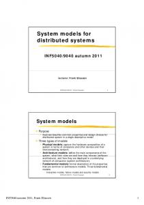
Fig. 1

Fig. 1. Flow diagram of the three-level discretization procedure.

3 Subdividing catchments into hydro-landscapes: cells to take into account the vertical structure of soil profiles (Haverkamp et al., 2004). a practical proposition iii) Finally, if required by the process conceptualisation 3.1 Principle of the hydro-landscape delineation and/or numerical considerations such as convexity requirement, a third discretization level can be used and the hydroAs mentioned in Sect. 1, for small catchments, landscape fealandscapes can be subdivided into smaller elements, the tures such as agricultural fields, buildings, and hedges can be modelling units. Note that heterogeneity within hydrorepresented explicitly, as well as the water pathways between landscapes can be taken into account in a statistical way usthem. We can even end up with standard partial differential ing for instance the “tile” approach (e.g. Koster and Suarez, equations. The conservation laws can be solved using appro1992) used in atmospheric sciences, if the geographical lopriate numerical methods, which are consistent with the excation of these heterogeneity is not important. Conservation change fluxes approach. At larger scales, such a representalaws can be solved on the obtained elementary volumes, with tion is not feasible and simplified representations are needed. various degrees of complexity. In the remaining of the section we focus on the second level The first discretization level (sub-catchments) is perof discretization and introduce a method providing rationales formed, using traditional terrain analysis, based on the Digfor the determination of hydro-landscapes units for medium ital Elevation Model. This level is not detailed in this paFig. 2 to large catchments. The principle of hydro-landscape is deper (for more details see Dehotin, 2007). The second disscribed in Fig. 2. The first step consists in the definition of cretization level (hydro-landscape) requires the used of difhomogeneous areas using the data set available. In a second ferent kinds of landscape data. The available data needed step, the homogeneous areas map is combined with the first to describe the landscape heterogeneity inside the model are level discretization map (sub-catchments), and with other characterized by different spatial resolutions. In addition, we vector maps required to represent hydrological processes to need to define hydro-landscape consistently with the charend up with the final hydro-landscape delineation. acteristic spatial and temporal scales of the represented hyHomogeneous zones delineation will be different accorddrological processes. In the next section we focus on this ing to the refinement needed in the heterogeneity description. second level discretization and introduce a method providing For small catchments where detailed data are often available rationales for the determination of hydro-landscapes units (e.g. agricultural fields), a simple combination of the availacross scales. The third discretization level can be required able data can be used for homogeneous zones definition (e.g. according to numerical constraints associated with the methMoussa et al., 2002; Rodriguez et al., 2005; Branger, 2007 ods used to represent hydrological processes. We present an – see also Sect. 5.3.). For medium and large scale catchillustration of the third discretization level in section 4. ments, some simplifications are needed. Usually, many mapping techniques such as smoothing are used. However, it’s difficult with these techniques to keep in the landscape relevant details that might be important for hydrological modelling. Moreover, these mapping procedures do not produce www.hydrol-earth-syst-sci.net/12/769/2008/

Hydrol. Earth Syst. Sci., 12, 769–796, 2008

776

J. Dehotin and I. Braud: Variability of input data Fig. 1

Fig. 2

Fig. 2. Flow diagram of hydro-landscape delineation.

any confidence about the final homogeneous zones map. In the remaining of the section, we present a methodology to derive homogeneous zones for medium to large catchments, based on classification techniques. 3.2

Subdividing medium to large catchments in homogeneous zones: classification requirements

Hydro-landscapes, introduced by Winter (2001), can be defined as areas where hydrological processes can be considered as homogeneous. They can be considered as an extension of the HRU concept or of the Representative Elementary Columns – RECs – proposed by Haverkamp et al. (2004). Their delineation can take into account what will be referred to as factors below, influencing hydrological processes, e.g. slope, land use, geology, pedology, etc. The choice of the retained factors depends on the modelling goal, and the considered hydrological processes. In general, the map obtained by the overlay of various GIS layers leads to a very fragmented picture (see Fig. 7d for example), which is not necessarily consistent with the variability of hydrological processes. For hydrological modelling this variability needs to be simplified. Traditional methods are based on smoothing techniques, which suppress the smallest units using area thresholds for instance. The results do not take into account the underlying hydrological processes, whereas the role of these small units can be very important. Improvements are therefore needed to end up with a more rational methodology. The discretization methodology should remain flexible enough to fit with objectives concerning the consistency of scales and the simplification of the patterns. Therefore, the method should allow a better control on the errors arising from the overlay of maps at different resolutions, in an objective and quantifiable way. Hydrol. Earth Syst. Sci., 12, 769–796, 2008

As a practical solution, we suggest to extend the principle of landscape classification, used is soil mapping for the definition of homogeneous areas. It allows defining different levels of complexity in landscape representation that can be associated with different levels of accuracy in hydrological processes description. The parameters used in the classification can be adapted to the dominant hydrological processes and the resolution of the final units remains consistent with the resolution of the available data. We borrowed the principles of our landscape classification from those used in soil mapping (Burrough et al., 1997) and more specifically from the method of Robbez-Masson (1994, 1995); RobbezMasson et al. (1999); Lagacherie et al. (2001). The latter is based on the definition of reference zones and an analysis of the neighbourhood composition at each location. 3.3

Homogeneous areas delineation principles using classification technique

The different steps of the homogeneous areas delineation method are the following: 1. Identification of the available data and their resolution. Various maps describing several catchment characteristics can be used as factors (slope, soil, lithology, landuse...). The classification is a raster-based method. Thus all maps must be in a raster format and are re-sampled with the same resolution, usually the finer one. Note that the procedure could stop here if the data are not sufficient to fulfil the objectives. 2. Choice of relevant hydrological processes and their representation according to the available data. www.hydrol-earth-syst-sci.net/12/769/2008/

J. Dehotin and I. Braud: Variability of input data 3. Definition of the p factors expected to be influential on these hydrological processes, according to the chosen representation. 4. Simplification of each factor into np classes. This is especially relevant for continuous data such as slope. Then the p factors maps are overlaid using GIS. This overlay leads to a map of the combined factors comP Q posed of a maximum of nj combined factors. One j =1

class is therefore a unique combination of the p factors. Up to this step, the procedure is therefore similar to the classical GIS layers overlay used for instance in the HRU approach. 5. Definition of the reference zones on the study catchment. They are areas associated with a unique combination of the retained factors, which can be related to a specific hydrological response, for instance a zone prone to saturated excess runoff. 6. Choice of a neighbouring window (size and shape) and of a descriptor of the composition of the combined factors within this neighbourhood. The neighbourhood window allows to relate each pixel to the pixels inside this window and thus to take into account its surrounding pixels to perform the classification. A descriptor of the pixels distribution within the neighbouring window is used to characterize each point (pixel) in the landscape. The reference zones are characterized using the same descriptor of the combined factors within each zone. 7. Mapping of the whole catchment using a pixel-by-pixel analysis. Each pixel is allocated to one of the reference zones according to a distance criterion between the descriptor of its neighbouring window composition and that of the reference zones. 8. Estimation of the distance map, which can be considered as a confidence map of the classification. 9. Iteration from steps 6 to 8 until a resolution ensuring a given accuracy and consistency with the input data is obtained. This step is important since the accuracy of the final map depends on the size of the neighbourhood window. Accuracy can be inferred using the confidence map. We present an illustration of the whole methodology in section 4 and will now detail steps 3 to 9 in Sects. 3.4 to 3.6. 3.4

Definition of landscape factors (step 3 to 4)

In natural sciences, there is not a unique definition of a “landscape” amongst disciplines. In agriculture, agro-landscape refers to an ensemble of fields that are classified according www.hydrol-earth-syst-sci.net/12/769/2008/

777 to natural vegetation, wooded zones, river network, topography and soil surface characteristics (Girard, 2000). In soil sciences, pedology is considered as the results of several interacting factors (climate, geology, slope, land use), which are used to define soil-landscapes. In ecology, eco-regions are defined as land and water extends including distinct natural community. For hydrology, the factors that will be retained in the analysis will depend on the modelled hydrological processes. To model infiltration, factors such as soil surface characteristics, soil types, management practices will be influential. To simulate runoff, we can consider topography, topographical index, and soil surface characteristics. For evapotranspiration modelling, land-use, orientation, groundwater levels (geology), snow melt (topography, orientation) can be taken into account. Once all needed factors are identified, their corresponding layers/maps superposition using GIS gives a composed picture of the landscape. This composed picture defines various combinations of the landscape factors characterizing the spatial organization and characteristics of water dynamics within the sub-catchment. 3.5

Definition of references zones (step 5)

The notion of reference zone has been borrowed from soil classification where Favrot (1989) proposed the use of reference sectors for small natural region characterisation. Reference zones are extensively surveyed areas that are supposed to contain all the soil classes of the region to be mapped. For the final cartography, one unique soil type characterizes each reference sector. The derivation of accurate classifications and the quantification of uncertainties has led to lots of research using techniques such as geostatistics, fuzzy sets, conditional probabilities (e.g. Burrough et al., 1997), the discussion of which is beyond the scope of the paper. We propose to extend the notion of reference area for hydrological purposes. We define a reference zone for hydrology as an area with a certain degree of homogeneity relevant in the characterisation of hydrological processes. It may correspond to a unique combination of factors or to a dominant combination of factors. For the modelling of evapotranspiration and runoff, such combination can be “deciduous forests over steep slopes” or “cultures over moderate slopes”. For modelling saturated zones and their influence on runoff, they can be “high topographic index” etc. Man influence can be included through management practices: “drained area”, “urban area”, etc. References zone can also be a particular natural region where water dynamics are specific (e.g. karstic areas, vineyard). There is no limitation in the number of reference zones considered in the analysis. Therefore, the modeller has a lot of flexibility in the mapping of the landscape heterogeneity (complex/simple description), according to the data available, their scale and its objectives. However, he keeps track of the choices he has made and of the hypotheses underlying the final maps. Hydrol. Earth Syst. Sci., 12, 769–796, 2008

778

J. Dehotin and I. Braud: Variability of input data ample provided in the left of Fig. 4, each colour of the pixels characterizes a specific combination of factors and we chose the histogram as a descriptor. To derive it we consider all the pixels inside the neighbourhood window (here a square) and count the number of each combination class (i.e. each colour) in this window. This histogram is constructed for each point of the map. The choice of the shape of the window allows taking into account some anisotropy in the catchment. For instance ellipsis neighbourhood window with the major axe oriented north south can be chosen if specific factor (e.g. topography) has such an orientation. 3.6.2

Fig. 3. Illustration of the neighbourhood Fig. 3 window’s definition.

If there is a good knowledge of the catchment, the reference zones can be quite easily defined and delineated using the a priori knowledge of field hydrologists. The latter can know the location of areas prone to saturation, or with high slopes, etc. For larger catchments or catchments where it is not possible to perform intensive field surveys, the task is more difficult. In this case, only the factors map can provide the available information. These maps can be used to define possible reference zones, according to traditional/standard knowledge about hydrological processes. In this case, a simplified classification of factors can be used and the reference zones can be defined using a statistical and spatial analysis of the multivariate map (see details in Sect. 4). The relevance of such delineation can then be confirmed by a specific field survey. 3.6 3.6.1

Mapping of homogeneous zones (steps 6 to 9) Neighbourhood definition and characterization of all point in the catchment (step 6)

“Landscape is what is around you” (Robbez-Masson, Foltête et al., 1999). With this Fig. sentence 4 these authors argue that the integration of spatial neighbourhood is necessary to describe the landscape. With this mapping approach, each point in the landscape is characterized by the composition of a neighbourhood window around the point (contextual analysis). The modeller must define the size and the shape of a neighbourhood window (e.g. ellipsis neighbourhood window on Fig. 3). The latter determines the resolution of the final units. All points in the catchment are characterized using the composition of their neighbourhood window. The characterization of each point is performed (inside the neighbourhood window) using a descriptor on the multivariate image (in pixels). The descriptor may be a histogram, a mean or a standard deviation. This descriptor is calculated for each of the points of the multivariate image. In the exHydrol. Earth Syst. Sci., 12, 769–796, 2008

References zones characterization and mapping procedure (steps 6 to 9)

Similarly for each point of the map the references zones are characterized by their composition, using the same descriptor, according to the combination factor map (right of Fig. 4). The mapping consists of assigning all points in the landscape the most similar reference zone in a statistical sense. Similarity is defined as the minimization of the distance between the descriptor of each characterized point and those of the references zones. The distance may be the modal distance, Kolmogorov distance or Manhattan distance (RobbezMasson, 1994). See the illustration of the principles in Fig. 4. The result of the mapping consists in two maps. The first map represents a segmentation of the initial multivariate image into elementary landscape units or polygons. This map is thus composed of homogeneous and unstructured areas. The second map can be considered as a confidence map for the classification. This map represents the distance between the descriptor (e.g. histogram) of each point and the affected reference zone descriptor (e.g. histogram). It quantifies the reliability of the modelling units by providing a criterion of the statistical quality of the classification. If the confidence map is not satisfactory, the classification can be improved by adding more reference zones to get a better representation of the landscape. 3.6.3

Scale and accuracy assessment (step 9)

The size of the hydro-landscapes in the final map depends of the size of the neighbourhood window. This size must be chosen in consistency with the resolution of the input data. The size of the smallest units on the classified map cannot be lower than the finest units of the input maps. An iterative procedure is therefore needed to define a neighbourhood window size, consistent with this first constraint. This iterative procedure consists in testing several sizes for the neighbourhood window until the constraint is fulfilled (iteration of steps 6 to 8). This ensures consistency of the modelling units with the input data resolutions. Once the “optimal” size of the neighbourhood windows is chosen, the classification can be improved using the distance www.hydrol-earth-syst-sci.net/12/769/2008/


Fig. 3

779

Fig. 4 Fig. 4. Basic principles for the mapping by landscape classification. On the left map is figured a point to be mapped (the black one) with a squared neighbourhood window and the composition histogram within this window. On the right map are shown the reference zones and their composition histograms. In the middle the Manhattan distance is used to search for the minimum distance between the left histogram and those of the reference zones.

map. The latter provides an idea of the accuracy of the classification. If the distance is large, it means that the similarity of the neighbourhood with the available reference zones is poor. Therefore, new references zones can be added in the areas with larger distances and used to improve the mapping (iteration of steps 6, 7 to 9). This will reduce uncertainties on the landscape heterogeneity representation and handling. 3.7

Determination of the hydro-landscapes and modelling meshes

As shown in Fig. 2, the hydro-landscapes are obtained by overlaying the map of homogeneous areas and the subFig. 5. Location of the upper-Saône catchment in France. catchments map. Other vector maps can be added at thisFig. 5 stage. These maps may describe hydrological discontinuities, or specific boundary maps, that are important for the In the next section, we present an illustration of the whole modelling. After this step, the discretization result consists methodology through the detailed presentation of a case of irregular polygons composing an unstructured mesh. Acstudy. For the determination of homogeneous areas, we also cording to the numerical method used for the representapresent a comparison with more traditional approaches. The tion of some processes, these meshes can be directly used goal of the comparison is to show which method produces as modelling units (e.g. vertical infiltration with one dimenthe “best” representation of the landscape heterogeneity. The sional Richard’s equations, or evaporation flux simulation). comparison through hydrological model results is beyond the In some other cases, such as the resolution of partial differscope of the paper and will be reported in other publications. ential equations using the finite volumes or finite elements method, these meshes cannot be directly used, because they are not convex. A third level of discretization is thus needed. 4 Illustration of the methodology using data from the This third level of discretization consists in deriving conupper-Saône catchment in France vexes meshes based on the hydro-landscapes of the second level of discretization. This can be obtained by forcing the In this section, we illustrate the discretization methodology hydro-landscapes polygons with Triangular Irregular Netpresented in Sect. 2.6 and summarised in Fig. 1 using data works (TINs) or by using specific algorithms to derive confrom the upper-Saône catchment, upstream of the gauging vex meshes from the hydro-landscapes. station Lechatelet (11 700 km2 ). It is located in north-eastern www.hydrol-earth-syst-sci.net/12/769/2008/


780


France (Fig. 5). The river rises in the Vosges Mountains in Lorraine, and flows south through Burgundy. The elevation ranges from 177 a.m.s.l. at the outlet to more than 1215 a.m.s.l. in the Vosges. The main land-use classes are broad-leaved forests, arable land, and pastures. The arable land is mainly located in the south-western part, whereas the pastures are located in the north-eastern part of the catchment. The forests are spread all over the catchment and in the Vosges, coniferous forest is important. Urban surfaces constitute about 2% of the catchment area with the largest concentration around the town of Dijon. The geology is characterised by limestone in the southern parts and sandstones and granites in the northern parts. We first present the available data and their resolution, as well as the objectives of the study. Then, we illustrate the nested discretization procedure of Fig. 1. For the definition of homogeneous areas, all the steps outlined in Sect. 3 are presented. The results of the classification are also compared with traditional procedures. 4.1

Available data and objectives of the modelling

The available data for this catchment include: – 3 h time resolution values of precipitation (rain and snow), potential evapotranspiration, and the maximum and minimum temperatures, distributed on 8×8 km grid for the period 01/08/1981–31/07/1998 and provided by Météo-France. – Daily stream flow data from the French hydrographic database (Banque Hydro) for the period 01/08/1981– 31/07/1998 at 22 gauging stations. Their catchment areas cover a wide spectrum ranging from 52 to 11 700 km2 . – A digital elevation model (DEM) with resolution 200 m, 100 m and 1000 m from the IGN (Institut Géographique National) in France and provided by Water Agency (Agence de l’eau). – The Corine Land Cover database provided by Institut Français de l’ENvironnement (IFEN) with a 500 m resolution. The database contains 44 land cover classes organized in three levels (Bossard et al., 2000). – A soil map from the Soil information system of France from National Institute of Agronomic Research (INRA) with a 1/1 000 000 resolution (Jamagne et al., 1995). For about one-third of the catchment, another soil database at 1/250 000 resolution was available from the IGCS (Inventaire Gestion et Conservation des Sols) lead by INRA (http://www.gissol.fr/ or http://www.igcs-stb. org/) – The geology map of France with a 1/1 000 000 resolution from the BRGM (Bureau de Recherche Géologique et Minières). Hydrol. Earth Syst. Sci., 12, 769–796, 2008

– A referential of groundwater systems from SANDRE specification (Secrétariat d’Administration Nationale des Données Relatives a` l’Eau) and available at the web site http://sandre.eaufrance.fr/. We can underline the large heterogeneity in the resolution of input maps. Furthermore, meteorological data, which determine the hydrological response, provide the coarser information, both in space and in time. These data are not used in the definition of the hydro-landscapes units, but the information should be taken into account in the choice of the processes representation and then in the final discretization. As shown in Fig. 1, the first step is to define the modelling objectives. The goal of our study is to evaluate the impact on the water cycle, of changes in the land-use. The target variables are the water balance components at the daily, monthly and annual time scales and for sub-catchments with a minimum size of about 50 km2 (the size of the smallest catchment where stream flow data is available, but also the order of magnitude for the meteorological data mesh). The following processes are considered: evapotranspiration, water transfer within the non-saturated and saturated zones, and river flow. No detailed representation of runoff is considered. Further details on the choice of the methods for the representation are given in Sect. 5.1. With these modelling objectives in mind, we used the various sources of information as follows for the spatial discretization of the catchment. First we used the DEM to extract the river network and delineate the sub-catchments (first discretization level, Sect. 4.2.1). For the determination of hydro-landscape units (second level of discretization and sub-catchment scale variability) we used the lithology, land use and slope maps (Sect. 4.2.2.), soil map and the groundwater referential. If required by the process representation and numerical constraints, further sub-divisions of hydrolandscape units can be performed (third level of discretization). For instance, hydro-landscape can be subdivided to get convex polygons for the application of finite volumes methods. 4.2

Catchment discretization for a distributed water balance components derivation

The first step in the discretization is to determine the subcatchments (Sect. 4.2.1). A large degree of heterogeneity, especially in land-use, is still present within each subcatchment. We assume that it must be taken into account for an accurate simulation of evapotranspiration and this justifies the determination of hydro-landscapes units and the use of a second level of discretization. The relevance of this choice should of course be proven through simulation, but it is beyond the scope of the paper, where we only wish to illustrate our methodology for landscape discretization, using the available data of the upper-Saône catchment. www.hydrol-earth-syst-sci.net/12/769/2008/


781

Fig. 6. Discretization of the catchment in sub-catchments using the first (a) and second (b) Strahler order.

Fig. 6 :

4.2.1

A first discretization into sub-catchments

The first discretization level was that of the sub-catchments. Sub-catchments were determined using DEM analysis and river network structure. Several algorithms were proposed to extract hydrological information from DEM (Peuker and Douglas, 1975; Martz and Garbrecht, 1992). We used the Tardem algorithm (Tarboton, 1997) to derive sub-catchments from the 200 m resolution DEM. The 200 m resolution DEM can be used because the modelling does not include a fine representation of runoff. The algorithm we used first performed a detection and treatment of depression zones in the DEM. Then the local direction of out-flows were calculated for each cell using the D8 algorithm. The contributing areas were determined for each cell in terms of drained area and a threshold area was used to define river cells. We used a vector file of the actual river network provided by the National Geographic Institute (France). The TARDEM algorithm allows to enforce the drainage direction to follow an existing river network (using DEM correction). In this case, the automatic network extracted from the DEM is the same as the existing river network used to force the drainage direction. The sub-basins drained by every link of the river network were delineated using a threshold for the Strahler order of the river links. Figure 6a and b show a discretization of the Saône catchment in sub-catchments using the first and second Strahler orders. The number of sub-catchments was 341 and 81 for the first and second order respectively, with an average area of 35 and 147 km2 respectively. These values were quite large but related to the fact that the existing network only considered permanent river reaches.

Table 1. Table defining the factors and the delimitation of classes for the whole classification. Land Use Urban areas Open spaces Agricultural areas Vineyards and fruit trees Pastures Sparsely vegetated areas Broad leaved-forest Coniferous forest Water body Slope Very low slope Low slope Moderate slope High slope Very high slope Lithology Old sediments Sediments Chalk Alluvium Sandstone Tertiary chalk Marl and clayey chalk Sand and clay

Fig. 7



Fig. 6 : 782


Fig. 7. Maps of (a) land-use, (b) slope and (c) lithology on the upper Fig. Saˆ 7 one catchment. (d) Map of the combination of the three previous factors. Superimposed is the discretization of the catchments into sub-catchments at the two Strahler order.

4.2.2

Catchment discretization into hydro-landscapes

Because of the catchment’s size, the available data and the modelling goal presented in Sect. 4.1, the hydro-landscape delineation requires the mapping of homogeneous areas (Fig. 2). In this section, we performed the homogeneous areas delineation using the method proposed in Sect. 3.3. Delineation of the homogeneous zones Factors definition and data selection The modelling objective was the determination of the distributed components of the water balance at various time scales. One of these components is evapotranspiration and we considered land-use as one of its controlling factors. We assumed that the partition of incoming rainfall between runoff and infiltration was controlled by factor such as lithology and slope. Other factors such as the topographic index of Beven and Kirkby (1979), as well as the direct use of soil-landscape units could have been considered. In the Hydrol. Earth Syst. Sci., 12, 769–796, 2008

example described below, we therefore considered three factors: lithology, slope and land-use. The next step was to simplify the information through the definition of classes for continuous data such as slope. In the case of the Saône, we reclassified the original 26 classes of the Corine Land cover map (resolution: 500 m), present in the catchment, into nine classes, especially because the distinction of the various urban areas was not useful for the study. This classification was corresponding to expected differences in hydrological response, especially evapotranspiration. In the same way we simplified the lithology map according to the parent material and the age of the layers, leading to seven classes for lithology (scale: 1/1 000 000). The slope map was derived from the DEM analysis discussed in Sect. 4.1 and classified into five classes (resolution: 200 m). The various classes for the different factors are given in Table 1. All the maps were re-sampled with a 200 m resolution and were used to define the map of combined factors. The maps of factors are shown in Fig. 7a, b and c. Figure 7d shows the multivariable image of the combined factors obtained after superposition of the three data layers. It is composed of 221


J. Dehotin and I. Braud: Variability of input data classes of combined factors (amongst the 9×5×7=315 possible classes) and formed the basis for the hydro-landscape mapping procedure. Figure 7d shows that the variability of these factors is large within a sub-catchment. It is an argument for considering this second level of discretization. Definition of the references zones The definition of reference zones may be the most difficult step of this approach. In an ideal case, reference zones should result from a good knowledge on the catchment (e.g. Peschke et al., 1999 for the definition of factors controlling infiltration excess and saturation excess areas). Usually, this is not the case, as for the upper-Saône catchment. Therefore, we chose to define references zones using spatial analysis of a simplified combination of landscape factors. This map was derived using the 9 classes for land-use, 2 classes for slopes (low and high) and 4 classes for lithology (see Table 1). They were used to define 46 types of reference zones (Table 2). Their location is shown in Fig. 8 and was defined by ensuring the representativeness of each reference zone in all areas over the catchment. As much as possible, we chose areas with a certain degree of homogeneity. Mapping procedure For the mapping procedure, we used an available software named CLAPAS developed by Robbez-Masson (1994) (http://www.umr-lisah.fr/Produits/Clapas/). It allows mapping using landscape classification techniques. Several descriptors of the neighbourhood are available: mean, standard deviation, histogram, and matrix of co-occurrence. The software proposes several choices of the neighbourhood window shape: square, ellipse, circle, ring etc. The squared neighbourhood window is usually used. We used a square, as particular anisotropy handling was not needed. The histogram of composition was used as descriptor (of neighbourhood window and references zones) and the Manhattan distance to compute the similarity with the composition of the reference zones. The choice of the Manhattan distance is justified since it is more robust than the other distances (Kolmogorov, Cramer, etc.) used for performing similarity between vectors (Robbez-Masson, 1994). Each point X within the catchment was characterized by a specific histogram of the possible combined factors (p=221) within the neighbourhood window, denoted by MX =(d1 , d2 , . . ., dp ). The histogram calculation was also performed for each k=46 references zones. For a reference zone j , the histogram is noted Mj =(m1j , m2j , . . ., mpj ). Affectation of a point X to a reference zone j consists of minimizing the Manhattan distance d(Mx , Mj ) calculated by Eq. (1); see Fig. 4:


783 Table 2. Table defining the reference zones type.

Numbers 1 2 3 4 5 6 7 8 9 10 11 12 13 14 15 16 17 18 19 20 21 22 23 24 25 26 27 28 29 30 31 32 33 34 35 36 37 38 39 40 41 42 43 44 45 46

Name of the reference zone Urban areas Open spaces on sedimentary soil with law slope Open spaces on chalky soil with law slope Open spaces on alluvium with low slope Open spaces on marl with low slope Open spaces on chalky soil with high slope Agricultural areas on sedimentary soil with low slope Agricultural areas on chalky soil with low slope Agricultural areas on alluvium with low slope Agricultural areas on marl with low slope Agricultural areas on sedimentary soil with high slope Agricultural areas on chalky soil with high slope Agricultural areas on alluvium with high slope Vineyard and fruit tree on sedimentary soil with low slope Vineyard and fruit tree on chalky soil with low slope Vineyard and fruit tree on marl with low slope Vineyard and fruit tree on sedimentary soil with high slope Vineyard and fruit tree on chalky soil with high slope Prairies on sedimentary soil with low slope Prairies on chalky soil with low slope Prairies on alluvium with low slope Prairies on marl with low slope Prairies on sedimentary soil with high slope Prairies on chalky soil with high slope Prairies on alluvium with high slope Sparsely vegetated areas on sedimentary soil with low slope Sparsely vegetated areas on chalky soil with low slope Sparsely vegetated areas on alluvium with low slope Sparsely vegetated areas on marl with low slope Sparsely vegetated areas on sedimentary soil with high slope Sparsely vegetated areas on chalky soil with high slope Broad leaved-forest on sedimentary soil with high slope Broad leaved-forest on chalky soil with high slope Broad leaved-forest on alluvium with high slope Broad leaved-forest on marl with high slope Broad leaved-forest on sedimentary soil with high slope Broad leaved-forest on chalky soil with high slope Broad leaved-forest on alluvium with high slope Coniferous forest on sedimentary soil with low slope Coniferous forest on chalky soil with low slope Coniferous forest on alluvium with low slope Coniferous forest on marl with low slope Coniferous forest on sedimentary soil with high slope Coniferous forest on chalky soil with high slope Coniferous forest on alluvium with high slope Water body

p X di − mij d(MX , Mj ) =

(1)

i=1

For the assessment of the “optimal” resolution of hydrolandscapes, we varied the neighbourhood windows size, iteratively from 3 km down to one kilometer.


784

J. Dehotin and I. Braud: Variability of input data that the average area of the map units dropped when the neighbourhood window decreased. When the neighbourhood window decreased, the map units were smaller, and the number of coarse features decreased. On Fig. 9 (right), we can see that the decrease of the neighbourhood window was leading to an improvement of the confidence map (less blue colour). Choice of the mapping that fits well with the input data

Fig. 8

Fig. 8. Map of the reference zones.

Resulting hydro-landscapes and distance maps In the first iteration, we used a neighbourhood windows resolution of 3 km. In a second iteration, we tried to refine the mapping by using a smaller neighbourhood window of 2.2 km. In a third step, we tested a window’s size of 1.4 km. Figure 9 shows the maps of the hydro-landscapes and their corresponding distance maps for three sizes of the neighbourhood window: 3, 2.2 and 1.4 km. In Fig. 9 (right), the yellow colour corresponds to pixels that are correctly classified (i.e. with a low value of the Manhattan distance) whereas the blue colour corresponds to pixel which are badly classified (high values of the Manhattan distance). Figure 10 shows the distribution of the area of the mapped units and Table 3 provides the corresponding statistics. Table 3 shows Hydrol. Earth Syst. Sci., 12, 769–796, 2008

The use of different sizes for the neighbourhood windows provided modelling units at different resolutions. The statistical analysis of the area distribution provided a way to assess the consistency of the results with the resolutions of the input data. The finest scale of the input data was 1/250 000 and the coarser scale was 1/1 000 000. The final modelling unit could not be more accurate than the finest scale. For a scale of the classified map of 1/250 000, the rule of “quart” states that the modelling units must have an area larger than 1/4th of 2.5×2.5 km2 , i.e. 1.6 km2 . For a scale of the classified map of 1/1 000 000, the units should be larger than 1/4th of 10×10 km2 , i.e. 6.4 km2 . The percentage of the cumulated areas occupied by the units with area lower than these two thresholds are provided in Table 3. A trade off is needed to choose the most appropriate map. The first one (top of Fig. 9) with an average area of 16 km2 seemed too coarse compared to the resolution of the input data. In the third map (bottom of Fig. 9) the average area of 5 km2 is consistent with a scale of 1/250 000 for the classified map. However this feeling of accuracy may be misleading because 18 % of the total area was composed of units with an area smaller than 6.4 km2 and about 6% of the total area was composed of units with area smaller than 1.6 km2 . The better compromise may be to choose the second map (middle, Fig. 9) with an average area around 9 km2 . More than 90% of the total area was covered with landscape units having an area larger than 6.4 km2 and more than 97% of the total area was covered with landscape units having an area larger than 1.6 km2 . Thus, the iterative procedure of this classification approach provided an efficient tool to assess the mapping resolution according to the input data resolution. Furthermore, the distance map provided an idea of the uncertainties on the modelling units representation, and could be used for uncertainty analysis. The final choice of the window size resolution can also be conditioned by sources of information, not taken into account in the classification procedure. For instance, in the case of the Saône catchment, the input rainfall was available on square grids of 64 km2 . Therefore, the first map resolution (Fig. 9, top left) could be more consistent with rainfall resolution for hydrological modelling. Other modelling objectives and/or other factors map resolution would produce different maps. We performed additional simulation to test the sensitivity of homogeneous zone mapping to the chosen factors. The mapping criteria were www.hydrol-earth-syst-sci.net/12/769/2008/


785

Table 3. Statistics of the areas of the mapped units for several sizes of the neighbourhood window.

Map 1 (3 km) Map 2 (2.2 km) Map 3 (1.4 km)

Average area (km2 )

Standard deviation of area (km2 )

% of the total area with units area lower than 1.6 km2


16 9 5

99 70 34

1 2.5 6

5 9.6 18.4

Fig. 9a

Fig. 9a. Left: hydro-landscapes units and Right: distance map for the neighbourhood window of 3 km.



786


Fig. 9b

Fig. 9b. Left: hydro-landscapes units and Right: distance map for the neighbourhood window of 2.2 km.

the same as those used for the middle map of Fig. 9. The reference zones were the same; the neighbourhood windows shape and size were also the same. The results (Fig. 10, left) were compared with the Fig. 9 (middle) map, (redrawn in Fig. 10, right). We performed two kinds of tests. In the first test, we replaced the slope map by the topographic index map. The result (Fig. 10a) shows that two new reference landscapes appeared: “Pasture on chalky soil” and “Agricultural areas on high slope”. On the other hand, the “Broad leaved-forest on chalky soil” disappeared. In the second test, the topographic index was added to the factors used for the mapping of Fig. 9 (slope, lithology, and land use). The result Hydrol. Earth Syst. Sci., 12, 769–796, 2008

(Fig. 10c) shows that the “Pasture on chalky soil” and the “Broad leaved-forest on chalky soil” were well represented in the final map. This example illustrates that, the choice of the factors retained in the analysis really influence the homogeneous zone mapping. The presented technique allows a large flexibility in landscape heterogeneity representation. It is likely to ensure a relevant representation of heterogeneity according to the available data (factors) and modelling objectives.



787

Fig. 9c

Fig. 9c. Left: hydro-landscapes units and Right: distance map for the neighbourhood window of 1.4 km.

Comparison with the usual mapping techniques for homogeneous areas delineation In this section, we present the results of two traditional mapping techniques to delineate homogeneous areas and compare them with those of the classification methodology presented before. Traditional mapping techniques are based on area threshold criteria. For the usual mapping techniques we used areas threshold criteria of 6.4 km2 and 1.6 km2 corresponding respectively to the minimum and maximum scale of input data. Exhaustive evaluation of the classifica-


tion methodology needs a comparison for a range of models, but we focus at this stage on the capacity of the method to represent efficiently landscape heterogeneity. We show that the methodology allowed handling in more rational manner the uncertainties of heterogeneity representation in distributed modelling. Mapping results with the basic smoothing techniques Smoothing techniques are used to simplify the multivariate factors maps (the map of Fig. 7d), based on the area


788


Fig. 10. Comparison between mapping units when using different factors. (a) Factors used: land use, topographic index and Fig.landscape 10 lithology. (c) Factors used: land use, topographic index, slope and lithology. (b, d) reference map units (redraw of Fig. 9 middle). Fig. 10

statistics of the areas of the mapped units can be found in Table 4. When areas with areas smaller than 6.4 km2 were removed, the average area of the map units was of about 255 km2 . Less than 0.04% of the total area was mapped with units having an area lower than 6.4 km2 (Fig. 12a). The mapped units were very coarse and the picture was not very satisfactory. When removing areas lower than 1.6 km2 (Fig. 12b), the average area of the units was of about 32 km2 and about 1% of the total area was covered with units having an area lower than 6.4 km2 . Fig. 11

Fig. 11. Fraction of the total area occupied with units landscapes of area lower than the area given in abscissa for three values of the neighbourhood window.

Mapping by re-sampling and smoothing technique

The final map of hydro-landscapes can be obtained by re-sampling the original multivariate map (the one shown in Fig. 7d) of the combination of factor in order to get a of the map units. Usually, the basic technique (we used the smoother image. For this re-sampling (we used the resamArcView smoothing function) consists in removing areas pling function of ArcView), only the desired final factors smaller than those representing the resolution of the input were considered (in our case the 46 factors retained for the Fig. 11 data. The corresponding maps are shown in Fig. 12 and the reference zones). Then the same smoothing technique as Hydrol. Earth Syst. Sci., 12, 769–796, 2008



789

Table 4. Synthetic Statistics of different mapping techniques and their capacity to keep in the final map suitable references zones: For 1/250 000 (Min Area = 1.6 km2 ) to 1/1 000 000 (Min Area = 6.4 km2 ).

Landscape Classification Basic smoothing technique Re-sampling technique

Average Area (km2 )



%Reference areas kept in the final map

9 14.6 15

2.5 0.4 1

9.6 6 8

76 28 43

(a)

(b) Fig. 12

Fig. 12. Mapping of the catchment derived from classical smoothing technique obtained by removing areas lower than (a) 6.4 km2 , (b) 1.6 km2 .

before was applied to this map. The corresponding maps are shown on Fig. 13 and the statistics of the area of the units are provided in Table 4.

automatically. In any case, with usual mapping techniques, only five to twenty percents of the 46 reference landscapes of Table 2 were represented in the final map (Table 4).

When removing areas smaller than 6.4 km2 , the average area of the map units was about 64 km2 and less than 8% of the total area was mapped with units having an area lower than 6.4 km2 (Fig. 13a). When removing areas smaller than 1.6 km2 , the average area of the map units was about 15 km2 and less than 1% of the total area was mapped with units having an area lower than 1.6 km2 (Fig. 13b).

When using re-sampling techniques, the result seemed visually better. But only 28 to 50% of the 46 reference landscapes were represented in the final map.

In the case of landscape classification, between 63 and 90% of the 46 reference landscapes types were represented in the final map (and more when new references were added). Thus, this technique provides better result than the classical method. It allows keeping suitable features in the Comments representation of the heterogeneity. (a) (b) In Table 4, we represent the percentages of the 46 iniDiscussion about the methods proposed for the homoFig. 13 tial reference zone encountered in the final map. We observe geneous zones determination a large difference between the three mapping techniques. The first basic smoothing technique does not allow keeping a Because classical mapping techniques use a threshold reliable representation of the landscape heterogeneity in the area, they are not efficient for keeping in the landscape representation, suitable features consistent with the available final map. More precisely, the urban zone, wine, agricultural and alluvial areas do not correspond to those present in the input data and represented hydrological processes. They do input data. When we decreased the minimum area, it was not offer any mechanism for map unit resolution handling. difficult to control the features in the landscape relevant for In any case, there is no quantification of uncertainties of the hydrological modelling, because small units were removed map units when these methods are used.



(a)

(b) Fig. 12

790


(a)

(b) Fig. 13

Fig. 13. Mapping of the hydro-landscapes derived by re-sampling into the 46 combined factors retained for the reference zones and removing areas of less than (a) 6.4 km2 , (b) 1.6 km2 .

The methodology presented in this paper for the derivation of homogeneous zones is a first attempt to derive something applicable in practice and allows keeping suitable details in the landscape. It also allows assessing uncertainties on each map units by providing a confidence map. Finally, it allows a large degree of flexibility in the landscape heterogeneity representation, while constraining the hydrologist to formalise the processes he wants to retain and represent within the modelling units. Nevertheless, we recognise that the method suffers from some arbitrary choices. This includes the choice of the factor maps, the definition of the classes used in the definition of the combination of factors maps, the delineation of the reference zones, the choice of the descriptor for heterogeneity description, the distance used for the classification. A complete sensitivity analysis of the consequences of these choices on the final map should be performed. But this is beyond the scope of the paper where our purpose was to illustrate the methodology outlined in Sect. 3 and initiate discussion about it. Another limitation of the method is linked to the use of raster-based formats, whereas lots of GIS layers are provided as vector maps. The method proposed for homogeneous zone determination is a simplification procedure of these GIS layers. This step can be omitted when the available data can be used directly (Fig. 2). In the last step of hydro-landscape delineation, other vector maps describing boundaries or linear features (sub-catchments, river network, ditches, hedges...) can be used to get the final polygons (see Sect. 4.2.2). Although the comparison with traditional methods shows that the classification technique we propose has the potential to better represent landscape heterogeneity (Sect. 4.2.3), the paper does not demonstrate that the proposed approach is “better” than the traditional use of grid squares or smoothing approach when computing the hydrology. An answer by Hydrol. Earth Syst. Sci., 12, 769–796, 2008

yes or not is probably not possible because verification data will often be insufficient to discriminate and assess the relevance of the various maps. Nevertheless we think that our method can be useful in many ways. By performing sensitivity analysis, it should be possible to get an idea of the refinement below, which results – for a given objective and data availability – are insensitive. It can also allow testing hypotheses about catchment functioning or preparing an experimental campaign by highlighting more sensitive zones or defining sampling strategies able to lower model uncertainties. Hydro-landscape determination Once the homogeneous areas were determined, we obtained the hydro-landscape by overlapping the sub-catchments map with the homogeneous areas map (bottom of Fig. 2). We also added the vector map of the hydro-geological system boundaries and of pedo-landscapes. This ensured that hydro-landscapes were also homogeneous in terms of hydraulic properties and that they were not crossing aquifer boundaries. Figure 14 show the final map of the hydro-landscape polygons. 4.2.3

Third level of discretization

Vertical hydrological processes such as evapotranspiration, vertical transfer within the unsaturated and water transfers in river reaches can be represented using directly the hydrolandscapes of Fig. 14. On the other hand, the representation of lateral water transfers in the saturated zone, for instance with the Boussinesq equation solved with finite volume or finite elements methods, cannot be performed without convex meshes. Figure 15 provides an example of a third level of discretization, which can be used to get convex elements from the hydro-landscape map of Fig. 14. In this illustration, www.hydrol-earth-syst-sci.net/12/769/2008/

Fig. 14


791

Fig. 15

Fig. 14

Fig. 14. Mapping of the hydro-landscapes derived on the Saône catchment. The different colours correspond to the sub-catchments, and the black lines represent the hydro-landscapes.

we used a regular hexagonal mesh as a basis. The latter was modified to fulfil the hydro-landscapes boundaries. The use of TINs would be another alternative. 4.3

Concluding remarks about the case study and the methodology

The paper is focused on the description of land surface heterogeneity but the latter cannot be disconnected from the climate forcing heterogeneity. In the case study, the spatial and temporal discretization of the climatic forcing (three-hourly Fig. 15is one of the most limiting data over 64 km2 grid squares) elements for the choice of the process representation. In a general manner, it is clear that any spatial discretization should be consistent with the input data and conversely that the input data, especially rainfall spatial and temporal resolution, should be adapted to the hydrological processes resolved within the model. Results of Arnaud et al. (2002) and Zehe et al. (2005) illustrate the importance of a proper description of rainfall for improving the simulation of hydrological models. After an extensive discussion about land surface discretization for hydrological models, the next section provides outlines of models, which are being constructed based on these hydro-landscapes. 5

Illustrations of models constructed using the discretization principles outlined in the paper

In this part, we present several examples to show how the discretization methods can be used for practical hydrological modelling. Using the discretization principles outlined in the paper, we are developing a modelling platform called LIQUID (Viallet et al., 2006), based on modularity of hydrologwww.hydrol-earth-syst-sci.net/12/769/2008/

Fig. 15. Example of a third level of discretization through a mapping of convex hydro-landscapes.

ical processes and appropriate spatio-temporal integration of processes. Once the modelling framework will be built, different tests will provide more precise advice on the suitability of a given catchment discretization for a given objective. We provide below some examples of scientific questions, the model designed to answer them and their corresponding spatial discretization. These examples span various catchment areas from 1 km2 to about 12 000 km2 and include the previous section illustration. All the models are built within the LIQUID framework. 5.1

First example: impact of land use change on the hydrological regime of a catchment of about 12 000 km2

The first example corresponds to the one presented in Sect. 4 (Fig. 5) on the upper Saône catchment (11 700 km2 ). As mentioned before, the modelling objective is to study the sensitivity of the long term (ten years) water balance of the catchment to modification of land use. Given the resolution of input rainfall (64 km2 and three hours), the size of the target catchments is about 50 km2 . The model includes the various components of the water balance: evapotranspiration and vertical transfer in the saturated/non-saturated zones are modelled using Varado et al. (2006b). River flow is modelled using the kinematic wave approximation. Previous studies had highlighted the role of groundwater on this catchment (Engeland et al., 2006). Thus, we built a module solving the 2D Boussinesq equation for water transfer within the saturated zone, able to cope with unstructured polygons (Dehotin, 2007). It can be applied on the hydro-landscapes geometry presented before (Fig. 14), providing that they are re-meshed to fulfil convexity constraints (third level of discretization, Fig. 15). This module has been coupled to the 1D saturated/unsaturated water transfer module using the facilities provided by the LIQUID framework. It provides the lateral flow to the 1D module, which in return provides the Hydrol. Earth Syst. Sci., 12, 769–796, 2008

792

J. Dehotin and I. Braud: Variability of input data Fig. 16

Fig. 16. Geometry used inFig. the16modelling of a 6 km2 subcatchment in the Cévennes-Vivarais region. Colours correspond to the pedolandscapes of the soil map, black contour lines correspond to the sub-catchment boundaries and blue lines to the river reaches.

Fig. 17

Fig. 17. Geometry used in the modelling of the La Fontaine du Theil catchment. Orange fields are drained fields, yellow fields are agricultural fields, green lines are hedges and blue lines are river reaches.

recharge to the groundwater (Dehotin, 2007). An “interface module” simulating groundwater/river interaction has also been designed. The fluxes are calculated based on the Miles (1985) approach. The complete model is still under construction and results will be reported in forthcoming papers.

simple model allowed us to distinguish areas prone to saturation excess and other prone to infiltration excess (Manus et al., 20082 ). Their delineation will be used to locate experimental sites for verification and validation of the hypotheses.

5.2

5.3

Second example: experimental design for the study of runoff generation in catchments of 1 to 100 km2 prone to flash-floods

The Cévennes region in South-East France is prone to heavy rainfall events leading to catastrophic flash-floods such as the one occurred on 8–9 September 2002 (Delrieu et al., 2005). The modelling objective is to design a future field study dedicated to the improvement of our knowledge on runoff generation for such heavy rainfall events. For this purpose, we perform sensitivity studies to quantify the impact of soil characteristics on the simulated runoff for the 8–9 September 2002. The model includes a first discretization level into small subcatchments of about 1 km2 (consistent with the resolution of radar rainfall products). Each sub-catchment is then divided into hydro-landscapes corresponding to the areas described in the pedological map in order to fully include soil variability (Fig. 16). The water transfer Fig. 17 within these pedological units is modelled using the same approach as before (Varado et al., 2006b) and the river flow routine is also the same. Ponding is directly transferred to the closest river reach with a flux calculated using the Manning Strickler equation. This Hydrol. Earth Syst. Sci., 12, 769–796, 2008

Third example: impact of hydrological discontinuities on the hydrology of small agricultural catchments

The objective of the study is to quantify the impact of agricultural features (hedges, ditches, drained fields, grassed strips) on the hydrology of a small agricultural catchment (La Fontaine du Theil, Brittany, France, 1.28 km2 ). In this case, hydro-landscapes are directly defined from the landuse map and the use of the method proposed in Sect. 3.3 for homogeneous areas delineation is not needed (Fig. 17). Agricultural fields, hedges, drained fields, and ditches and river reaches are considered as independent objects. The hydrological behaviour of each element is modelled using various modules based on more or less complex principles. Water transfer within agricultural fields is modelled using the approach of Varado et al. (2006b), based on the solution of the 1D Richards equation, including possible ponding at the 2 Manus, C., Braud, I., Vandervaere, J. P., Viallet, P., and Anquetin, S.: A modelling approach to assess the sensitivity of runoff generation mechanisms to soil characteristics in the context of Mediterranean extreme events, Hydrol. Earth Syst. Sci., in preparation, 2008.


J. Dehotin and I. Braud: Variability of input data soil surface, a sink term for root extraction and a source/sink term for lateral transfer within the saturated zone. In drained fields, the saturated level and the partition of rainfall between infiltration and runoff are modelled using a simplified approach (Branger et al., 20083 ). A module derived from the TNT2 model of Beaujouan et al. (2002) was designed to represent the influence of a hedge on water infiltration (Branger, 2007). The water flow routing within the river is based on the kinematic wave approximation of the St Venant equation. Lateral transfer in the saturated zone between agricultural fields, agricultural field and hedges is modelled using an “interface module” which estimates the flux based on the Darcy law and the hydraulic head difference between the centroids of each element. The river receives contributions directly from the drained field and from the ponding of the fields adjacent to it. Sensitivity tests comparing simulations with or without the activation of this “interface module” show that the global model is performing as expected by transferring water from the upstream areas to the downstream, consistently with the topography (Branger, 2007). This work will be extended to study the impact of the hydrological discontinuities on pesticide transfer.

6

Conclusions and perspectives

In this paper, starting from existing knowledge and practice, we proposed rationales for a better handling of land surface heterogeneity in distributed hydrological models. We proposed to use nested discretization with a resolution governed by the objectives of the modelling, data availability and resolution and hydrological processes representation. The first level is defined using sub-catchments organised along the river network. If required by the objectives and hydrological processes variability, a second level of discretization, called hydro-landscapes, can be used to take into account the variability described through various GIS layers. Finally, a third level of discretization is proposed to fulfil geometrical constraints linked to linear features and/or numerical schemes. In the second part of the paper, we detailed the second step: the derivation of hydro-landscapes and proposed a flexible methodology, based on landscape classification for medium to large catchments. The methods allows to better take into account the differences in data resolution and provide a confidence map of the classification which can further be used for sensitivity and uncertainty assessment. As outlined by Holland et al. (2007), a sensitivity study of model results to the definition of the geometry should be performed, in the same way it is usually done for model parameters. The methodology proposed in this paper provides guidelines for the building of such a sensitivity study. 3 Branger, F., Tournebize, J., Carluer, N., Kao, C., Vauclin, M.,

and Braud, I.: A conceptual modeling approach for pesticide transport in a tile-drained field, Agr. Wat. Man., submitted, 2008.


793 We hope that the ideas expressed in this paper will stimulate research in various domains connected to hydrological modelling. Paraphrasing Beven (2006) about uncertainties, we could consider surface heterogeneity as an opportunity to develop new fields of research instead of considering it a “problem”. As shown in this paper, if we take surface heterogeneity into account, we end up with unstructured meshes, which do not even hold the convexity properties, necessary to use existing classical numerical schemes. There is an opportunity for applied mathematicians to work with hydrologists in order to develop methods applicable on these meshes. One promising example is that of the tRiBS model (Ivanov et al., 2004a) developed using triangular irregular networks, customized to handle hydrological specificities such as catchment boundaries, river network or the requirement to a better discretization along river flat areas where saturated zones can be expected. The inclusion of linear discontinuities (river reaches, hedges, ditches, dikes) is also a promising area of research to derive methods able to i) describe properly these networks, ii) take them into account into hydrological models explicitly at small scales iii) derive simplified parameterisations for use in larger catchment scale models iv) describe the organisation of these networks within the landscape, to be able to take them into account as sub-grid scale parameterisations. For larger catchments, as the Saône catchment presented in this paper, the methodology we proposed is only a first step. We hope that specialists in landscape typology or laws of organization would be interested in taking possession of the subject in order to improve the methodology. The question of spatialization of soil hydraulic properties over the modelling units remains also an open question, deserving research investment. A closer collaboration between pedologists and hydrologists, as proposed by Lin et al. (2006) is a necessary step towards the study of such questions. Acknowledgements. The authors thank Lionnel Bargeot and Jérôme Gourmelon from ENESAD in Dijon for fruitful discussion about soil classification and for their assistance in using the Clapas software. Flora Branger and Claire Manus are thanked for providing Figs. 15 and 16 respectively. Christian Puech and anonymous reviewers are thanked for their constructive comments, which helped improving the quality of the paper. Edited by: R. Moussa

References Abbott, M. B., Bathurst, J. C., Cunge, J. A., O’Conell, P. E., and Rasmusson, J.: An introduction to the European Hydrological System-Syst‘eme Hydrologique Europ’een “SHE” 1: History and philosophy of a physically based distributed modeling system, J. Hydrol., 87, 45–59, 1986a. Abbott, M. B., Bathurst, J. C., Cunge, J. A., O’Connell, P. E., and Rasmussen, J.: An introduction to the European Hydrological System – Syst‘eme Hydrologique Europ’een, ”SHE”, 2, Struc-


794 ture of a physically-based, distributed modelling system, J. Hydrol., 87, 61–77, 1986b. Argent, R. M.: An overview of model integration for environmental applications–components, frameworks and semantics, Environ. Modell. Software, 19(3), 219–234, 2004. Arnaud, P. and Lavabre, J.: Coupled rainfall model and discharge model for flood frequency estimation, Water Resour. Res., 38(6), 1075, doi:10.1029/2001WR000474, 2002. Beaujouan, V., Durand, P., Ruiz, L., Aurousseau, P., and Cotteret, G. : A hydrological model dedicated to topography-based simulation of nitrogen transfer and transformation: rationale and application of the geomorphology-denitrification relationship, Hydrol. Process., 16(2), 493–507, 2002. Beldring, S.: Multi-criteria validation of a precipitation-runoff model, J. Hydrol., 257, 189–211, 2002. Beldring, S., Gottschalk, L., Seibert, J., and Tallaksen, L. M.: Distribution of soil moisture and groundwater levels at patch and catchment scales, Agric. Forest Meteorol., 98–99, 305–324, 1999. Bergkamp, G.: A hierarchical view of the interactions of runoff and infiltration with vegetation and microtopography in semiarids shrublands, Catena, 33, 201–220, 1998. Beven, K.: How far can we go in distributed hydrological modeling, Hydrol. Earth Syst. Sci., 5, 1–12, 2001, http://www.hydrol-earth-syst-sci.net/5/1/2001/. Beven, K.: Towards an alternative blueprint for a physically-based digitally simulated hydrological modelling system, Hydrol. Process., 16, 189–206, 2002a. Beven, K.: Towards a coherent philosophy for modelling the environment, Proc. R. Soc. London A, 458, 2465–2484, 2002b. Beven, K.: On environmental models of everywhere on the GRID, Hydrol. Process., 17, 171–174, 2003. Beven, K.: On undermining the science, Hydrol. Process., 20, 3141–3146, 2006. Beven, K. and Binley, A.: The future of distributed models: model calibration and uncertainty prediction, Hydrol. Process., 6, 279– 298, 1992. Beven, K. and Kirkby, M. J.: A physically-based variable contributing area model of basin hydrology, Hydrol. Sci. Bull., 24, 43–69, 1979. Blöschl, G. and Sivapalan, M.: Scales issues in hydrological modelling – a review, Hydrol. Process., 9(3–4), 251–290, 1995. Boorman, D. B., Hollis, J. M., and Lilly, A.: Hydrology of soil types: a hydrologically-based classification of the soils of the United Kingdom, Inst. Hydrol., Wallingford, http://www.ceh.ac. uk/products/publications/hydrology.html, 1995. Bossard, M. Feranec, J., and Otahel, J.: Corine land cover technical guide – Addendum 2000, Technical report No. 40, European Environment Agency, Copenhagen, Denmark, 2000. Branger, F.: Prise en compte des discontinuités hydrologiques dans le transfert de pesticides: utilisation d’une plate-forme de modélisation hydrologique pour la construction de modules spécifiques et l’intégration d’un modèle de bassin versant, Application au bassin versant de la Fontaine du Theil, Université Joseph Fourier, Grenoble I, Grenoble, France, 2007. Braud, I., Vich, A., Zuluaga, J., Fornero, L., and Pedrani, A.: Vegetation influence on runoff and sediment yield in the Andes region: observation and modelling, J. Hydrol., 254, 124–144, 2001. Burrough, P., van Gaans, P., and Hootsmans, R.: Continuous classi-


J. Dehotin and I. Braud: Variability of input data fication in soil survey: spatial correlation, confusion and boundaries, Geoderma, 77(2–4), 115–135, 1997. Carluer, N. and De Marsily, G.: Assessment and modelling of the influence of man-made networks on the hydrology of a small watershed: implications for fast flow components, water quality and landscape management, J. Hydrol., 285(1–4), 76–95, 2004. Cerdan, O., Le Bissonnais, Y., Govers, G., Lecomte, V., van Oost, K., Couturier, A., King, C., and Dubreuil, N.: Scale effect on runoff from experimental plots to catchments in agricultural areas in Normandy, J. Hydrol., 299, 4–14, 2004. Ciarapica, L. and Todini, E.: TOPKAPI: a model for the representation of the rainfall-runoff process at different scales, Hydrol. Process., 16(2), 207–229, 2002. De Condappa, D.: Etude de l’écoulement d’eau a` travers la zone non-saturée des aquifères de socle a` l’échelle spatiale du bassin versant, Application a` l’évaluation de la recharge au sein du bassin versant de Maheshwaram, Andhra Pradesh, Inde, Université Joseph Fourier, Grenoble, France, 22 Avril 2005, 355 pp., 2005. Dehotin, J.: Prise en compte de l’hétérogénéité spatiale des surfaces continentales dans la modélisation hydrologique spatialisée, Application au Haut-bassin de la Saône, Thèse de l’Institut National Polytechnique de Grenoble, France, 254 pp., 2007. Delrieu, G., Ducrocq, V., Gaume, E., Nicol, J., Payrastre, O., Yates, E., Kistetter, P. E., Andrieu, H., Ayral, P. A., Bouvier, C., Creutin, J. D., Livet, M., Anquetin, S., Lang, M., Neppel, L., Obled, C., Parent-du-Chatelet, E., Saulnier, G.-M., Walpersdorf, A., and Wobrock, W.: The catastrophic flash-flood event of 8–9 September 2002 in the Gard region, France: a first case study for the Cévennes-Vivarais Mediterranean hydrometerorological observatory, J Hydrometeorol., 6(2), 34–52, 2005. D’Herbes, J. M. and Valentin, C.: Land surface conditions of the Niamey region: ecological and hydrological implications, J. Hydrol., 189(1–4), 18–42, 1997. Durand, Y., Brun, E., Mérindol, L., Guyomarch, G., Lesaffre, B., and Martin, E.: A meteorological estimation of relevant parameters for snow models, Ann. Glaciol., 18, 65–71, 1993. Eder, G., Sivapalan, M., and Nachtnebel, H. P.: Modelling water balances in an Alpine catchment through exploitation of emergent properties over changing time scales, Hydrol. Process., 17, 2125–2149, 2003. Engeland, K., Braud, I., Gottschalk, L., and Leblois, E.: Multiobjective regional modelling, J. Hydrol., 327(3–4), 339–351, 2006. Fan, Y. F. and Bras, R. L.: On the concept of a representative elementary area in catchment runoff, Hydrol. Process., 9, 821–832, 1995. Favrot, J. C.: Une stratégie d’inventaire cartographique a` grande e´ chelle: la méthode des secteurs de référence, Sciences du sol, 27, 351–368, 1989. Flügel, W. A.: Delineating Hydrological Response Units by Geographical Information System analyses for regional hydrological modelling using PRMS/MMS in the drainage basin of the river Bröl in Germany, Hydrol. Process., 9(3–4), 423–436, 1995. Gineste, P.: Télédétection spatiale et modélisation du fonctionnement hydrologique des petits bassins versants, Proceedings of the international workshop, organized by LCT – CEMAGREF – ENGREF ORSTOM, Water report 16 – FAO, 1997. Girard, M.: Glossaire de science du sol, Institut National


J. Dehotin and I. Braud: Variability of input data Agronomique de Paris-Grignon, 2000. Gottschalk, L., Beldring, S., Engeland, K., Tallakse, L., Saelthun, N. R., Kolberg, S., and Motovilov, Y.: Regional/macroscale hydrological modeling: a Scandinavian experience, Hydrol. Sci. J. – Journal des Sciences Hydrologiques, 46, 963–982, 2001. Grayson, R., Moore, I., and McMahon, T.: Physically based hydrologic modelling 1: A terrain-based model for investigative purposes, Water Resour. Res., 28(10), 2639–2658, 1992a. Grayson, R. B., Moore, I. D., and McMahon, T. A.: Physically based hydrologic modelling 2. Is the concept realistic, Water Resour. Res., 28(10), 2659–2666, 1992b. Green, A. E., Astill, M. S., McAneney, K. J., and Nieveen, J. P.: Path-averaged surface fluxes determined from infrared and microwave scintillometers, Agric. Forest Meteorol., 109(3), 233– 247, 2001. Grésillon, J. M.: Contribution a` l’étude de la formation des e´ coulements de crue sur les petits bassins versants, Approches numériques et expérimentales a` différentes e´ chelles. Habilitation a` Diriger des Recherches, Université Joseph Fourier, Grenoble, 1994. Haverkamp, R., Angulo-Jaramillo, R., Braud, I., Debionne, S., De Condappa, D., Gandola, F., Roessle, S., Ross, P., Sander, G., Vachaud, G., Varado, N., Viallet, P., and Zin, I.: POWER – Planner Oriented Watershed modelling system for Environmental Responses- Final Integrated report AgriBMPwater Project UE no. EVK1-CT-1999-00025, 26 pp., 2004. Holland, E. P., Aegerter, J. N., Dytham, C., and Smith, G. C.: Landscape as a model: the importance of geometry, PLOS Computational Biology, 3(10), e200, doi:10.1371/journal.pcbi.0030200, 2007. Ivanov, V. Y., Vivoni, E. R., Bras, R. L., and Entekhabi, D.: Catchment hydrologic response with a fully distributed triangulated irregular network model, Water Resour. Res., 40(11), W11102, doi:10.1029/2004WR003218, 2004a. Ivanov, V. Y., Vivoni, E. R., Bras, R. L., and Entekhabi, D.: Preserving high-resolution surface and rainfall data in operational-scale basin hydrology: a fully-distributed physically-based approach, J. Hydrol., 298(1–4), 80–111, 2004b. Jamagne, M., Hardy, R., King, D., and Bornand, M.: La base de données géographiques des sols de France, Etude et Gestion des Sols, 2, 153–172, 1995. Jothityangkoon, C., Sivapalan, M., and Farmer, D. L.: Process controls of water balance variability in a large semi-arid catchment: downward approach to hydrological model development, J. Hydrol., 254, 174–198, 2001. Klemes, V.: Conceptualisation and scale in hydrology, J. Hydrol., 65, 1–23, 1983. Koster, R. D. and Suarez, M. J.: Modeling the land surface boundary layer in climate models as a composite of independent vegetation stands, J. Geophys. Res, 97(D3), 2697–2715, 1992. Krause, P., Kralisch, S., and Flügel, W. A.: Preface: Model integration and development of modular modelling systems, Adv. Geosci., 4, 1–2, 2005, http://www.adv-geosci.net/4/1/2005/. Lagacherie, P., Cazemier, D. R., van Gaans, P. F., and Burrough, P. A.: Fuzzy k-means clustering of fields in an elementary catchment and extrapolation to a larger area, Geoderma, 77(2–4), 197– 216, 1997. Lagacherie, P., Robbez-Masson, J. M., Nguyen-The, N., and


795 Barthes, J. P.: Mapping of reference area representativity using a mathematical soilscape distance, Geoderma, 101(3–4), 105–118, 2001. Leavesley, G. H., Markstrom, S. L., Restrepo, P. J., and Viger, R. J.: A modular approach to addressing model design, scale, and parameter estimation issues in distributed hydrological modelling, Hydrol. Process., 16(2), 173–187, 2002. Lee, H., Sivapalan, M., and Zehe, E.: Representative Elementary Watershed (REW) approach: a new blueprint for distributed hydrologic modeling at the catchment scale: development of closure relations, in: Predictions ungauged streamflow in the Mackenzie river basin: today’s techniques and tomorrow solutions, edited by: Spence, C., Pomeroy, J., and Pietroniro, A., Canadian Water Resources Association (CWRA), Ottawa, Canada, 165–218, 2005. Lehmann, P., Hinz, C., McGrath, G., Tromp-van Meerveld, H. J., and McDonnell, J. J.: Rainfall threshold for hillslope outflow: an emergent property of flow pathway connectivity, Hydrol. Earth Syst. Sci., 11, 1047–1063, 2007, http://www.hydrol-earth-syst-sci.net/11/1047/2007/. Lin, H., Bouma, J., Pachepsky, Y. A., Western, A. W., Thompson, J., van Genuchten, M. T., Vogel, H.-J., and Lilly, A.: Hydropedology: synergetic integration of pedology and hydrology, Water Resour. Res., 42, W05301, doi:05310.01029/02005WR004085, 2006. Martz, L. and Garbrecht, J.: Numerical definition of drainage network and subcatchment areas from digital elevation models, Comp. Geosci., 18(6), 747–761, 1992. Miles, J. C.: The representation of flows to partially penetrating rivers using groundwater flow models, J Hydrol., 82, 314–355, 1985. Motovilov, Y. G., Gottschalk, L., Engeland, K., and Rodhe, A.: Validation of a distributed hydrological model against spatial observations, Agric. Forest Meteorol., 98–99, 257–277, 1999. Moussa, R., Voltz, M., and Andrieux, P.: Effects of the spatial organization of agricultural management on the hydrological behaviour of a farmed catchment during flood events, Hydrol. Process., 16(2), 393–412, 2002. Mroczkowski, M., Raper, G. P., and Kuczera, G.: The quest for more powerful validation of conceptual catchment models, Water Resour. Res., 33(10), 2325–2335, 1997. Neitsch, S. L., Arnold, J. G., Kiniry, J. R., and Williams, J. R.: Soil and Water Assessment Tool, SWAT 2000. Theoretical documentation, 542 pp. http://www.brc.tamus.edu/swat/doc.html, 2005. Palacios-Velez, O. L. and Cuevas-Renaud, B.: Automated rivercourse, ridge and basin delineation from digital elevation data, J. Hydrol., 86, 299–314, 1986. Parde, M.: Fleuves et rivières, Collection Armand Colin, Paris, 224 pp., 1955. Peschke, G., Etzenberg, C., Töpfer, J., and Zimmermann, S.: Runoff generation regionalization: analysis and a possible approach to a solution, IAHS Publications, 254, 147–156, 1999. Peuker, T. and Douglas, D. H.: Detection of surface-specific points by local parallel processing of discrete terrain elevation data, Comput. Graphics Image Process, 4, 375–387, 1975. Puech, C.: Utilisation de la télédétection et des modèles numériques de terrain pour la connaissance du fonctionnement des hydrosystèmes, Institut National Polytechnique de Grenoble, Grenoble, France, 105 pp., 2002.


796 Refsgaard, J. C., Henriksen, H. J., Harrar, W. G., Scholten, H., and Kassahun, A.: Quality assurance in model based water management – review of existing practice and outline of new approaches, Environ. Modell. Software, 20(10), 1201–1215, 2005. Reggiani, P. and Rientjes, T. H. M.: Flux parameterization in the Representative Elementary Watershed approach: application to a natural basin, Water Resour. Res., 41, W04013, doi:04010.01029/02004WR003693, 2005. Reggiani, P. and Schellekens, J.: Modelling of hydrological responses: the representative elementary watershed approach as an alternative blueprint for watershed modelling, Hydrol. Process., 17, 3785–3789, 2003. Reggiani, P., Sivapalan, M., and Hassanizadeh, S. M.: A unifying framework for watershed thermodynamics : balance equations for mass, momentum, energy and entropy, and the second law of thermodynamics, Adv. Water Resour., 22(4), 367–598, 1998. Reggiani, P., Sivapalan, M., Hassanizadehb, S. M., and Gray, W. G.: A unifying framework for watershed thermodynamics: constitutive relationships, Adv. Water Resour., 23(1), 15–39, 1999. Reggiani, P., Sivapalan, M., and Hassanizadeh, S. M.: Conservation equation governing hillslope response : exploring the physical basis of water balance, Water Resour. Res., 36(7), 1845–1863, 2000. Robbez-Masson, J. M.: Reconnaissance et délimitation de motifs d’organisation spatiale. Application a` la cartographie des pédopaysages, PhD Thesis, Ecole Nationale Supérieure Agronomique de Montpellier, 191 pp., 1994. Robbez-Masson, J. M., Foltête, J. C., Cabello, L., et al.: Prise en compte du contexte spatial dans l’instrumentation de la notion de paysage, Application a` une segmentation assistée, Revue internationale de géomatique, 9, 173–195, 1999. Rodriguez, F., Morena, F., and Andrieu, H.: Development of a distributed hydrological model based on urban databanks – production processes of URBS, Water Sci. Technol., 52(5), 241–248, 2005. Sauquet, E., Krasovskaia, I., and Leblois, E.: Mapping mean monthly runoff pattern using EOF analysis, Hydrol. Earth Syst. Sci., 4, 79–93, 2000, http://www.hydrol-earth-syst-sci.net/4/79/2000/. Sauquet, E.: Mapping mean annual river discharges: geostatistical development for incorporating river network dependency, J. Hydrol., 331(1–2), 300–314, 2006. Schneider, M. K., Brunner, F., Hollis, J. M., and Stamm, C.: Towards a hydrological classification of European soils: preliminary test of its predictive power for the base flow index using river discharge data, Hydrol. Earth Syst. Sci., 11, 1501–1513, 2007, http://www.hydrol-earth-syst-sci.net/11/1501/2007/. Seguis, L., Cappelaere, B., Peugeot, C., and Vieux, B.: Impact on Sahelian runoff of stochastic and elevation-induced spatial distributions of soil parameters, Hydrol. Process., 16(2), 313–332, 2002. Sidle, R. C.: Field observation and process understanding in hydrology: essential components in scaling, Hydrol. Process., 20, 1439–1445, 2006. Sivapalan, M.: Prediction in ungauged basins: a grand challenge for theoretical hydrology, Hydrol. Process., 17, 3163–3170, 2003. Skoien, J. and Blöschl, G.: Catchments as space-time filters: a joint spatio-temporal geostatistical analysis of runoff and precipita-


J. Dehotin and I. Braud: Variability of input data tion, Hydrol. Earth Syst. Sci., 10, 645–662, 2006, http://www.hydrol-earth-syst-sci.net/10/645/2006/. Skoien, J. O., Blöschl, G., and Western, A. W.: Characteristic space scales and timescales in hydrology, Water Resour. Res., 39(10), 1034, doi:10.1029/2002WR001736, 2003. Tarboton, D. G.: A new method for the determination of flow directions and contributing areas in Grid Digital Elevation models, Water Resour. Res., 33(2), 309–319, 1997. Tian, F., Hu, H., Lei, Z., and Sivapalan, M.: Extension of the Representative Elementary Watershed approach for cold regions via explicit treatment of energy related processes, Hydrol. Earth Syst. Sci., 10, 619–644, 2006, http://www.hydrol-earth-syst-sci.net/10/619/2006/. Varado, N., Braud, I., Galle, S., Le Lay, M., Séguis, L., Kamagate, B., and Depraetere, C.: Multicriteria assessment of the Representative Elementary Watershed approach on the Donga catchment (Benin) using a downward approach of model complexity, Hydrol. Earth Syst. Sci., 10, 427–442, 2006a, http://www.hydrol-earth-syst-sci.net/10/427/2006/. Varado, N., Braud, I. and Ross, P. J.: Development and assessment of an efficient numerical solution of the Richards’ equation including root extraction by plants, J. Hydrol., 323, 258–275, 2006b Vertessy, R., O’Loughlin, E., Beverly, E., and Butt, T.: Australian experiences with the CSIRO Topog model in land and water resources management, in: Proceedings of UNESCO International Symposium on Water Resources Planning in a Changing World, Karlsruhe, Germany, June 28–30, 1994, III-135-144 pp., 1994. Viallet, P., Debionne, S. Braud, I., Dehotin, J., Haverkamp, R., Sâadi, Z., Anquetin, S., Branger, F., and Varado, N.: Towards multi-scale integrated hydrological models using the LIQUID framework, Proceedings of the 7th International Conference on Hydroinformatics 2006, 4–8 September, Nice, France, Vol. I, 542–549, 2006. Viaud, V., Durand, P., Mérot, P., Sauboua, E., and Saädi, Z.: Modeling the impact of the spatial structure of a hedge network on the hydrology of a small catchment in a temperate climate, Agric. Water Manage., 74(2), 135–163, 2005. Viney, N. and Sivapalan, M.: A framework for scaling of hydrologic conceptualizations based on a disaggregation-aggregation approach, Hydrol. Process., 18, 1395–1408, 2004. Vivoni, E. R., Ivanov, V. Y., Bras, R. L., and Entekhabi, D.: Generation of triangulated irregular networks based on hydrologic similarity, J. Hydrol. Eng., 9, 288–302, 2004. Vogel, H.-J. and Roth, K.: Moving through scales of flow and transport in soil, J. Hydrol., 272(1–4), 95–106, 2003. Winter, T. C.: The concept of hydrological landscapes, J. Am. Water Resour. Assoc., 37(2), 335–349, 2001. Wood, E. F., Sivapalan, M., Beven, K., and Band, L.: Effects of spatial variability and scale with implication to hydrologic modeling, J. Hydrol., 102, 29–47, 1988. Zhang, G., Fenicia, F., Rientjes, T. H. M., Reggiani, P., and Savenije, H. H. G.: Modeling runoff generation in the Geer river basin with improved model parameterizations to the REW approach, Phys. Chem. Earth, 30, 285–296, 2005. Zehe, E., Becker, R., Bardossy, A., and Plate, E.: Uncertainty of simulated catchment runoff response in the presence of threshold processes: Role of initial soil moisture and precipitation, J. Hydrol., 315(1–4), 183–202, 2005.


Which spatial discretization for distributed hydrological models ...

Which spatial discretization for distributed hydrological models ...

Suggest Documents

Which spatial discretization for which distributed ... - HAL-INSU

Evaluating Three Hydrological Distributed Watershed Models ... - MDPI

Calibration of SWAT Hydrological Models in a Distributed Environment ...

ATHYS: a hydrological environment for spatial ... - Hydrologie.org

Research Article Methodology for Developing Hydrological Models ...

Scaling soil moisture for hydrological models - Hydrologie.org

Research Article Analysis of Spatial Discretization ...

Hydrological models are mediating models - hessd

System models for distributed systems

Spatial Discretization Methods for Air Gap Permeance ... - IEEE Xplore

Sampled 3D models for Cultural Heritage: which

Physically based distributed hydrological model calibration ... - HESS

Distributed Access to a Hydrological Administrative

A coupled distributed hydrological-stability analysis - hessd

On Spatially Distributed Hydrological Ecosystem ... - Water Accounting

A coupled distributed hydrological-stability analysis - hessd

Flood management using a distributed hydrological ...

Distributed Spatial Semantics

Temporal and spatial variation of hydrological ...

The prediction of hillslope flow paths for distributed hydrological ...

SWAT-CUP for Calibration of Spatially Distributed Hydrological ...

SWAT-CUP for Calibration of Spatially Distributed Hydrological ...

Integrating a distributed hydrological model and SEEA-Water for ...

Input data resolution analysis for distributed hydrological modeling