Wholistic Engineering for Software Reliability

Wholistic Engineering for Software Reliability ISSRE 2000 Tutorial Yashwant K. Malaiya Colorado State University • [email protected] • http://www.cs.colostate.edu/testing/ 10/13/00

1 ISSRE’00 Y.K. Malaiya

Wholistic Engineering for Software Reliability

Outline • • • • • •

Why it’s time… Demarcating, measuring, counting: definitions Science & engineering of reliability growth Those pesky residual defects Components & systems The toolbox

10/13/00


1

Why It’s Time: Emergence of SRE • Craft: incremental intuitive refinement • Science: why it is so – Observe, hypothesize, assess accuracy

• Engineering: how to get what we want – Approximate, integrate, evaluate

• Are we ready to engineer software reliability?

10/13/00


Why it’s time .. • We have data on different aspects of reliability to have reasonable hypotheses. • We know limitations of the hypotheses. • We will always need more data and better hypotheses … • We have enough techniques & tools to start engineering. 10/13/00


2

Why It’s Needed Now • • • • •

Reliability expectations growing fast Large projects, little time Quick changes in developing environments Reliance on a single technique not enough Pioneering work has already been done.

10/13/00


Learning from Hardware Reliability • Well known , well established methods • Now standard practice • Used by government and industrial org worldwide • Considered a hard science compared with software reliability

10/13/00


3

Hardware Reliability: The Status (1) • Earliest tube computers: MTTF comparable to some computation times! • 1956 RCA TR-1100: component failure rate models • 1959: MIL-HDBK-217A: common failure rate: 0.4x10-6 for all ICs for all cases • Revised about every 7 years 10/13/00


Hardware Reliability: The Status (2) • 1995 Final update: MIL-HDBK-217F, Notice 2. Still widely used. • Failure rates predicted often higher by a factor of 2-4, occasionally by an order of magnitude. • Constant failure-rate, the bathtub curve, the Arrhenius relationship have been questioned.

10/13/00


4

Hardware Reliability: The Status (3) • Why use hardware reliability prediction? – Feasibility Study: initial design – Compare Design Alternatives: Reliability along with performance and cost – Find Likely Problem Spots- high contributors to the product failure rate – Track Reliability Improvements

10/13/00


Hardware vs Software Reliability Models

Parameters

Hardware Past experience Past experience with with similar units similar units Software

Past experience* Early: past experience with similar units with similar units Later: from the same unit * Also suggested: from the same unit

10/13/00


5


Outline • • • • • •


10/13/00


Basic Definitions • Defect: requires a corrective action • Defect density: defects per 1000 noncomment source lines. • Failure intensity: rate at which failures are encountered during execution. • MTTF (mean time to failure): inverse of failure intensity 10/13/00


6

Basic Definitions (2) Limited use in SRE

• Reliability – R(t)=p{no failures in time (0,t)}

• Transaction reliability: probability that a single transaction will be executed correctly. • Time: may be measures in CPU time or some measure of testing effort. 10/13/00



Outline • • • • • •


10/13/00


7

Static and Dynamic Modeling • Reliability at release depends on – Initial number of defects (parameter) – Effectiveness of defect removal process (parameter) – Operating environment • Static modeling: estimate parameters before testing begins – Use static data like software size etc. • Dynamic modeling: estimate parameters during testing – Record when defects are found etc. – Time or coverage based

10/13/00


What factors control defect density? • Need to know for – static estimation of initial defect density – Find room for process improvement

• Static defect density models: • Additive (ex: Takahashi-Kamayachi) • D=a1f1+a2f2+a3f3… • Multiplicative (ex. MIL-HDBK-217, COCOMO, RADC) • D=C.F1(f1).F2(f2).F3(f3)…

10/13/00


8

A Static Defect Density Model Phase

• Li, Malaiya, Denton (93, 97)

Programming Team Process Maturity

• D=C.Fph.Fpt.Fm.Fs.Frv

Structure

• C is constant of proportionality, based on prior data. • Default value of each function (submodel) is 1. • Calibration based on past, similar projects 10/13/00

Requirement Volatility


Submodel: Phase Factor Fph • Based on Musa, Gaffney, Piwowarski et al.

At beginning of phase

Multiplier

Unit testing

4

Subsystem testing

2.5

System testing

1 (default)

Operation

0.35

10/13/00


9

Submodel: Programming Team Factor Fpt • Based on Takahashi, Kamayachi. Decline by 14% per year up to seven years.

Team’s average skill level Multiplier High

0.4

Average

1 (default)

Low

2.5

10/13/00


Submodel: Process Maturity Factor Fm • Based on Jones, Keene, Motorola data.

SEI CMM Level

Multiplier

Level 1

1.5

Level 2

1 (default)

Level 3

0.4

Level 4

0.1

Level 5

0.05

10/13/00


10

Submodel: Structure Factor Fs • Assembly code fraction: assuming assembly has 40% more defects • Factor=1+0.4×fraction in assembly • Module size: research reported at ISSRE 2000! • Complexity: Complex modules are more fault prone, but there may be compensating factors.

10/13/00


Submodel: Requirement volatility Factor Fph • Degree of changes and when they occur • Most impact when changes occur near the end of testing • Malaiya & Denton: ISSRE 99

10/13/00


11

Using the Defect Density Model • Calibrate submodels before use using data from a project as similar as possible. • Constant C can range between 6-20 (Musa). • Static models are very valuable, but high accuracy is not expected. • Useful when dynamic test data is not yet significant.

10/13/00


Static Model: Example For an organization, C is between 12 and 16. Average team and SEI maturity level is II. About 20% of code in assembly. Other factors are average (or same as past projects). Estimate defect density at beginning of subsystem test phase. •Upper estimate=16×2.5×1×1×(1+0.4 ×0.2)×1=43.2/KSLOC •Lower estimate= 12x2.5x1x1x(1+0.4x0.2)x1=32.4/KLOC

10/13/00


12

Test methodologies •Static (review, inspection) vs. dynamic (execution) •Test views •Black-box (functional): input/output description •White box (structural): implementation used •Combination: white after black •Test generation •Partitioning •Random/Antirandom/Deterministic •Input mix 10/13/00


Input Mix: Operational Profile • Need to do – find bugs fast? – estimate operational failure intensity? • Best mix for efficient bug finding (Li & Malaiya) – Quick & limited testing: Use operational profile – High reliability: Probe input space evenly • Operational profile will not execute rare and special cases – In general: Use combination • For acceptance testing: Need Operational profile

10/13/00


13

Operational Profile • Profile: set of disjoint actions, operations that a program may perform, and their probabilities of occurrence. • Operational profile: probabilities that occur in actual operation – Begin-to-end operations & their probabilities – Markov: states & transition probabilities • There may be multiple operational profiles. • Accurate operational profile determination may not be needed.

10/13/00


Operational Profile Example • “Phone follower” call types (Musa) A

Voice call

0.74

B

FAX call

0.15

A1

Voice call, no pager, answer

0.18

C

New number entry

0.10

A2

Data base audit

0.009

Voice call, no pager, no answer

0.17

D E

Add subscriber

0.0005

A3

Voice call, pager, voice answer

0.17

F

Delete subscriber

0.000499

A4

0.12

G

Hardware failure recovery

0.000001

Voice call, pager, answer on page

A5

Voice call, pager, no answer on page

0.10

10/13/00


14


Outline • • • • • •


10/13/00

9:54 AM


Modeling Reliability Growth • Testing cost can be 60% or more • Careful planning to release by target date • Decision making using a software reliability growth model (SRGM). Obtained using – Analytically using assumptions – Based on experimental observation

• A model describes a real process approximately • Ideally should have good predictive capability and a reasonable interpretation 10/13/00


15

A Basic SRGM • Testing time t, CPU execution time, man-hours etc.

• Total expected faults detected by time t: µ(t) • Failure intensity λ (t ) =

d µ (t ) dt

• Defects present at time t: N(t) −

dN ( t ) = β 1N (t) dt

10/13/00


A Basic SRGM (Cont.) • Parameter β1 is given by: β 1=

K 1 (S .Q. ) r

• S: source instructions, • Q: number of object instructions/r source instruction, • r: object instruction execution rate of the computer • K: fault-exposure ratio, range 1x10-7 to 10x10-7, (when t is in CPU seconds) 10/13/00


16

A Basic SRGM (Cont.) • We get

N(t) = N( 0 ) e- β 1t

µ (t) = β o (1 - e- β t ) 1

λ(t) = β o β 1 e-β t 1

• Where βo=N(0), total faults that would be eventually detected • Assumes no new defects are generated during debugging. • “Exponential model”: Jelinski-Muranda ‘71, Shooman ‘71, Goel-Okumoto ‘79 and Musa ‘75-’80.

10/13/00


SRGMs (Log Poisson) • Many SRGMs have been used. • Logarithmic model, by Musa-Okumoto, found to have a good predictive capability

µ (t) = β o ln(1 + β 1 t)

λ(t) =

βoβ1 1+ β 1t

• applicable as long as m(t) < N(0). In practice almost always satisfied. • parameters βo and β1 don’t have a simple interpretation. A useful interpretation by Malaiya and Denton.

10/13/00


17

Bias in SRGMs Average Error Average Bias

40 30 20 10 0 -10

Log

Inv Poly

Expo

Power

S-shaped

-20 -30 -40

•Malaiya, Karunanithi, Verma (’90) 10/13/00


SRGM: Preliminary Planning • Example: – – – – –

initial defect density estimated 25 defects/KLOC 10,000 lines of C code computer 70 million object instructions per second fault exposure ratio K estimated to be 4x10-7 Estimate the testing time for defect density 2.5/KLOC

• Procedure: – Find β0, β1 – Find testing time t1

10/13/00


18

SRGM: Preliminary Planning (cont.) • From exponential model

β o = N( 0 ) = 25x10 = 250 defects, β1=

10/13/00

K

4.0 x 10 -7

= 1 1 (S.Q. ) 10,000 x 2.5 x r 70 x 106 = 11.2 x 10-4 per sec


SRGM: Preliminary Planning (cont.) • Reliability at release depends on N( t1 ) 2.5 x 10 = = exp( −11.2 x10 − 4.t1 ) N(O) 25 x 10

t1 =

- ln(0.1) = 2056 sec . (CPU time) 11.2 x 10-4

λ( t1 ) = 250 x 11.2 x 10 -4 e-11.2 x 10 = 0.028 failures/ sec

-4

10/13/00

answer

t1


19

SRGM: Preliminary Planning (cont.) • For the same environment, β1.S is constant.

– Prior 5 KLOC project β1 was 2x10-3 per sec. – New 15 KLOC project, β1 can be estimated as 2x10-3/3 = 0.66x10-3 per sec.

• Value of fault exposure ratio (K) may depend on initial defect density and testing strategy (Li, Malaiya ’93).

10/13/00


SRGM: During Testing • Collect and pre-process data: – To extract the long-term trend, data needs to be smoothed – Grouped data: test duration intervals, average failure intensity in each interval.

• Select a model and determine parameters: – past experience with projects using same process – exponential and logarithmic models often good choices – model that fits early data well, may not have best predictive capability – parameters estimated using least square or maximum likelihood – parameter values used when stable and reasonable

10/13/00


20

SRGM: During Testing (cont.) • Compute how much more testing is needed: – fitted model to project additional testing needed • desired failure intensity • estimated defect density

– recalibrating a model can improve projection accuracy – Interval estimates can be obtained using statistical methods.

10/13/00


Example: SRGM with Test Data CPU Hours Failures

27 16 11 10 11 7 2 5 3 1 4 7

30

failure intensity per hour

1 2 3 4 5 6 7 8 9 10 11 12

25 20 15 10 5 0 0

5

10

15

CPU Hours

•Target failure intensity 1/hour (2.78.10-4 per sec.) 10/13/00


21

Example: SRGM with Test Data (cont.) • Fitting we get βo = 101.47 and β1 = 5.22 x 10-5

• stopping time tf is then given by: 2.78 x 10 -4 = 101.47 x 5.22 x 10 -5 e-5.22 x 10

-5

xtf

• yielding tf = 5 6, 4 73 sec., i.e. 15.69 hours

10/13/00


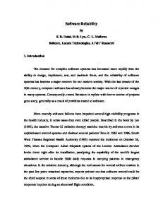
Example: SRGM with Test Data (cont.) Figure 1: Using an SRGM

0.008 0.007

Fitted model

failure intensity

0.006

measured values

0.005 0.004

Failure intensity target

0.003 0.002 0.001 0 0

5

10

15

20

Hours

10/13/00


22

Example: SRGM with Test Data (cont.) • Accuracy of projection: – – – –

Experience with Exponential model suggests estimated βo tends to be lower than the final value estimated β1 tends to be higher true value of tf should be higher. Hence 15.69 hours should be used as a lower estimate.

• Problems: – test strategy changed: spike in failure intensity • smoothing

– software under test evolving - continuing additions • Drop or adjust early data points 10/13/00



Outline • • • • • •


10/13/00


23

Test Coverage & Defect Density: Yes, they are related. •Defect vs. Test Coverage model, 1994: •Malaiya, Li, Bieman, Karcich, Skibbe •Estimation of number of defects, 1998 •Li, Malaiya, Denton

10/13/00


Motivation Why is Defect Density Important? • Important measurement of reliability • Often used as release criteria Beginning Of Unit Testing 16

10/13/00

Release Frequently Highly Cited Tested 2.0 0.33

NASA 0.1


24

Modeling : Defects, Time, & Coverage

10/13/00


Coverage Based Defect Estimation • Coverage is an objective measure of testing – Directly related to test effectiveness – Independent of processor speed and testing efficiency

• Lower defect density requires higher coverage to find more faults • Once we start finding faults, expect coverage vs. defect growth to be linear

10/13/00


25

Coverage Model, Estimated Defects µ(C) 95%

Defects

Linear Approximation after the knee

0

10

20

30

40

50

60

70

80

90

100

Cove rage

µ (C ) = A0 + A1C , C > Cknee • Only applicable after the knee • Assumptions : Logarithmic Poisson Model for defects and coverage elements. Stable Software 10/13/00


Location of the knee

Cknee

 Emin   D0 1 −   Dmin E0 

• Based on interpretation through logarithmic model • Location of knee based on initial defect density • Lower defect densities cause knee to occur at higher coverage • Parameter estimation : Malaiya and Denton (HASE ‘98) 10/13/00


26

Data Sets Used Vouk and Pasquini • Vouk data – from N version programming project to create a flight controller – Three data sets, 6 to 9 errors each

• Pasquini data – Data from European Space Agency – C Program with 100,000 source lines – 29 of 33 known faults uncovered 10/13/00


Defects vs. Branch Coverage Data Set: Pasquini 50

45

40

Defects Expected 35

Defects

30

25

20

Fitted Model 15

10

5 Model

Data

0 20

24

28

32

36

40

44

48

52

56

60

64

68

72

76

80

84

88

92

96

100

Branch Coverage

10/13/00


27

Defects vs. P-Use Coverage Data Set: Pasquini 60

50

Defects Expected

Defects

40

30

20

Fitted Model

10

Model

Data

0 20

24

28

32

36

40

44

48

52

56

60

64

68

72

76

80

84

88

92

96

100

P-Use Coverage

10/13/00


Estimation of Defect Density • Estimated defects at 95% coverage, for Pasquini data • 28 faults found, and 33 known to exist Measure Block Branch P-uses 10/13/00

Coverage Expected Achieved Defects 82% 36 70% 44 67% 48 56 ISSRE’00 Y.K. Malaiya

28

Defects vs. P-Use Coverage Data Set: Vouk 3 14

12

Defects Expected

10

Fitted Model

Defects

8

6

4

2

Model

Data

0 36

40

44

48

52

56

60

64

68

72

76

80

84

88

92

96

100

P-Use Coverage

10/13/00

57

ISSRE’00 Y.K. Malaiya

Coverage Based Estimation Data Set: Pasquini et al 60

50

Defects

40

Estimates are stable

30

20

10 Defects

1218

1157

1098

1037

976

914

853

792

733

672

611

549

488

427

368

307

246

184

123

2

62

0

Test Cases

10/13/00


29

Current Methods • Development process based models allow for a priori estimates – Not as accurate as methods based on test data

• Sampling methods often assume faults found as easy to find as faults not found – Underestimates faults

• Exponential model – Assume applicability of exponential model – We present results of a comparison 10/13/00


The Exponential Model Data Set: Pasquini et al 30

Estimate rises as new defects found 25

Defects

20

15

Estimates very close to actual faults 10

5

Estimate

Defects Found

1221

1160

1101

979

1040

917

856

795

736

675

614

552

491

430

371

310

249

187

126

5

65

0

Test Cases

10/13/00


30

Recent Conformation of Model • Frankl & Iakouneno, Proc. SIGSOFT ‘98 – 8 versons of European Space Agency program, 10K LOC – Single fault reinsertion

• Tom Williams, manuscript 1999 – analysis from first principles

10/13/00


Observations and Conclusions • Estimates with new method are very stable – Visual confirmation of earlier projections

• Which coverage measure to use? – Stricter measure will yield closer estimate

• Some code may be dead or unreachable – Found with compile or link time tools – May need to be taken into account 10/13/00


31


Outline • • • • • •


10/13/00


Reliability of Multi-component Systems • Software system: number of modules. • Individual modules developed and tested differently: different defect densities and failure rates. – Sequential execution – Concurrent execution – N-version systems 10/13/00


32

Sequential execution • Assume one module executed at a time. • fi: fraction of time module i under execution; λi its failure rate • Mean system failure rate: n

λ sys = ∑ f i λ i i=1

10/13/00


Sequential Execution (cont.) • T: mean duration of a single transaction • module i is called ei times during T, each time executed for duration di

f i= 10/13/00

ei • d i T

di T

i called 3rd time


33

Sequential Execution (cont.) • System reliability Rsys = exp(-λsys T) n

R sys = exp(- ∑ ei d i λ i ) i=1

• Since exp(-diλi) is Ri, n ei R sys = ∏ ( Ri ) i=1 10/13/00


Concurrent execution • Concurrently executing modules: all run without failures for system to run • j concurrently executing modules

time

m

λ sys = ∑ λ j j=1

10/13/00


34

N-version systems • Critical applications, like defense or avionics • Each version is implemented and tested independently • Common implementation uses triplication and voting on the result

10/13/00


N-version Systems (Cont.) Rsys=1-(1-R)3-3R(1-R)2 A B C

10/13/00

R=0.9 ⇒ Rsys=.972

Good Good

Good V

Bad


35

N-version systems: Correlation • Correlation significantly degrades fault tolerance • Significant correlation common in Nversion (Knight-Leveson) • Is it cost effective?

10/13/00


N-version systems: Correlation • 3-version system • q3: probability of all three versions failing for the same input. • q2: probability that any two versions will fail together. • Probability Psys of the system failing

P sys = q3 + 3 q 2 10/13/00


36

N-version systems: Correlation • Example: data collected by KnightLeveson; computations by Hatton • 3-version system, probability of a version failing for a transaction 0.0004 • in the absence of any correlated failures 2 2 P sys = (0.0004 ) + 3(1 - 0.0004)(0.0004 )

= 4.8 x 10 -7 10/13/00


N-version systems: Correlation • Uncorrelated improvement factor of 0.0004/4.8 x 10-7 = 833.3 • Correlated: q3 = 2.5×10-7 and q2 = 2.5×10-6 • Psys = 2.5×10-7 + 3.2.5×10-6 = 7.75×10-6 • improvement factor: 0.0004/7.75×10-6= 51.6 • state-of-the-art techniques can reduce defect density by a factor of 10 10/13/00


37

Safety • Analyze system to identify possible conditions leading to unsafe behavior. • Eliminate or reduce the probability of occurrence of such events. • Safety involves only a part of the system functionality.

10/13/00

11:58 AM


Fault Tree Analysis Top Event

Top Event

Gate

AND

Intermediate event

E

Gate

OR

Consequence

Deductive (reverse) logic

D

C

Causes (A,B,C,D) Basic events

10/13/00

A

B

Cut Sets: (A,C,D) (B,C,D) PTE=PAPCPD+ PBPCPD - PAP BPCPD 76 ISSRE’00 Y.K. Malaiya

38

Using Fault Trees • Deterministic analysis: prove that occurrence of unsafe events implies a logical contradiction. Feasible for small programs. • Probabilistic analysis: compute probability of occurrence of an unsafe event. Software, hardware and human factors. 10/13/00


Hazard Criticality Index Matrix Frequent

Probable

Occasional

Remote

Improbable Impossible

Catastrophic

1

2

3

4

9

12

Critical

3

4

6

7

12

12

Marginal

5

6

8

10

12

12

Negligible

8

11

12

12

12

12

Risk = frequency (events/unit time)× severity (detriment/event) Example from Navy 1986 10/13/00


39

Hazard Probability Frequent

MTBHUL Probability 0

MTBH: Mean time to hazard, UL: Unit life Compare with MIL-STD-882D App.A 10/13/00



Outline • • • • • •


10/13/00


40

Tools For Automating Software Reliability Engineering • Can we eliminate debugging? • Bugs would occur even with formal methods like VDM and Z [McGibbon] • hardware design and test: tools is now regarded to be mandatory • Software: increasing dependence 10/13/00


Why Tools Will be Mandatory

Defect Density/KLOC

Reliability expectations rising steadily 9 8 7 6 5 4 3 2 1 0 1970

1980

1990

2000

2010

Year

Source: Poston & Sexton 10/13/00


41

Software Testing Tools: History

• • • • •

70s: LINT: picks out all the fuzz 74: code instrumentor JAVS for coverage 80s: capture-replay etc. 92: Memory leak defectors Late 90s: Y2K tools

10/13/00


Manual vs. automated testing (QAI) Test step

Manual testing

Automated testing

Percent Improvement

Test plan development

32

40

-25%

Test case development

262

117

55%

Test execution

466

23

95%

Test result analyses

117

58

50%

Defect tracking

117

23

80%

Report creation

96

16

83%

Total hours

1090

277

75%

10/13/00


42

Tools for all Phases • Requirements phase Tools – Requirement Recorder/Verifier – Test Case Generation

• Programming Phase Tools (Static tools) – Metrics Evaluators – Code Checkers: – Inspection Based Error Estimation

10/13/00


Tools for all Phases (cont.) • Testing Phase Tools – – – – – –

10/13/00

Capture-Playback Tool Memory Leak Detectors Test Harness: Coverage Analyzers Load/performance tester Bug-tracker


43

Tools for all Phases (cont.) • Testing Phase Tools (cont.) – Defect density estimation – Reliability Growth Modeling tools – Coverage based Reliability Tools – Fault tree analysis – Markov reliability Evaluation

10/13/00


Static parameter estimation (planning)

Test case generation Test cases

Requirement s phase

Design phase

Coding phase

Requirement verifier

Inspection based bug estimation

Metrics

To unit testing

Checker Test cases

Test cases

Unit testing

Bug tracker

Integration test

System test

Configuration management

Acceptanc e test

Regression testing

Test harness Capture/replay

Load/stress testing

Coverage

10/13/00

Reliability growth models, coverage models


44

Tool Costs • • • • • • •

Tool identification Tool acquisition Tool installation/maintenance Study of underlying principles Familiarity with operation Risk of non-use Contacting user groups/support

10/13/00


References • J. D. Musa, A. Ianino and K. Okumoto, Software ReliabilityMeasurement, Prediction, Applications, McGraw-Hill, 1987. • Y. K. Malaiya and P. Srimani, Ed., Software Reliability Models, IEEE Computer Society Press, 1990. • A. D. Carleton, R. E. Park and W. A. Florac, Practical Software Measurement, Tech. Report, SRI, CMU/SEI-97-HB-003. • P. Piwowarski, M. Ohba and J. Caruso, ``Coverage Measurement Experience during Function Test,’’ Proc. Int. Conference on Software Engineering, 1993, pp. 287-301. • Y. K. Malaiya, N. Li, J. Bieman, R. Karcich and B. Skibbe ``The Relation between Test Coverage and Reliability ,‘’ Proc. IEEE-CS Int. Symposium on Software Reliability Engineering, Nov. 1994, pp. 186195.

10/13/00


45

References • Y.K. Malaiya and J. Denton, ``What do the Software Reliability Growth Model Parameters Represent,’’ Proc. IEEE-CS Int. Symposium on Software Reliability Engineering ISSRE, Nov. 1997, pp. 124-135. • M. Takahashi and Y. Kamayachi, ``An Emprical study of a Model for Program Error Prediction,’’ Proc. Int. Conference on Software Engineering, Aug. 1995, pp. 330-336. • J. Musa, Software Reliability Engineering’’, McGraw-Hill 1999. • N. Li and Y. K. Malaiya, ``Fault Exposure Ratio: Estimation and Applications,’’ Proc. IEEE-CS Int. Symposium on Software Reliability Engineering, Nov. 1993, pp. 372-381. • N. Li and Y. K. Malaiya, ``Enhancing accuracy of Software Reliability Prediction,’’ Proc. IEEE-CS Int. Symposium on Software Reliability Engineering, Nov. 1993, pp. 71-79.

10/13/00


References • P.B. Lakey and A. M. Neufelder, System and Software Reliability Assurance Notebook, Rome Lab, FSC-RELI, 1997. • L. Hatton, ``N-version Design Versus One Good Design’’ IEEE Software, Nov./Dec. 1997, pp. 71-76. • Tom McGibbon, “An Analysis of Two Formal methods VDM and Z, http//www.dacs.dtic.mil, Aug. 13, 1997. • Robert Poston, “A Guided Tour of Software Testing Tools,” Aonix, March 30, 1998. • M.R. Lyu Ed., Software Reliability Engineering, McGraw-Hill, 1996.

10/13/00


46

Wholistic Engineering for Software Reliability

Wholistic Engineering for Software Reliability

Suggest Documents

Improving Software Reliability using Software Engineering ... - CiteSeerX

Reliability Engineering Reliability Engineering

aspect-oriented software reliability engineering

web software reliability engineering - Gnedenko Forum

Reliability-oriented software engineering: design, testing and ...

7D4 Research in Software Reliability Engineering

13. on designing learning objects for a software reliability engineering ...

Software Reliability Engineering for System Test and ...

Hypertext for Software Engineering

yoga for a wholistic personality

Software Reliability - Google Sites

Reliability and Availability Engineering

Software Reliability - Semantic Scholar

Software Engineering for Practiced Software Enhancement

Software Reliability

Nissan Increases Software Reliability

software reliability simulation - CiteSeerX

Software Engineering for Computational Science and Engineering

Software abstractions for many- core software engineering

Software Reliability - Semantic Scholar

Reliability Prediction Basics - Reliability Engineering Basics

Software Engineering Techniques - AG Software Engineering - Uni ...

Software Engineering Research What Is Software Engineering ...

Software process simulation for reliability ... - Semantic Scholar