of training, choice of features, use of updating, impostor practice, and ....
evaluation, while systematically varying the factors among the selected values.
Data.
Why Did My Detector Do That?! Predicting Keystroke-Dynamics Error Rates Kevin Killourhy and Roy Maxion Dependable Systems Laboratory Computer Science Department Carnegie Mellon University 5000 Forbes Ave, Pittsburgh, PA 15213 {ksk,maxion}@cs.cmu.edu
Abstract. A major challenge in anomaly-detection studies lies in identifying the myriad factors that influence error rates. In keystroke dynamics, where detectors distinguish the typing rhythms of genuine users and impostors, influential factors may include the algorithm itself, amount of training, choice of features, use of updating, impostor practice, and typist-to-typist variation. In this work, we consider two problems. (1) Which of these factors influence keystroke-dynamics error rates and how? (2) What methodology should we use to establish the effects of multiple factors on detector error rates? Our approach is simple: experimentation using a benchmark data set, statistical analysis using linear mixed-effects models, and validation of the model’s predictions using new data. The algorithm, amount of training, and use of updating were strongly influential while, contrary to intuition, impostor practice and feature set had minor effect. Some typists were substantially easier to distinguish than others. The validation was successful, giving unprecedented confidence in these results, and establishing the methodology as a powerful tool for future anomaly-detection studies. Keywords: anomaly detection; keystroke dynamics; experimental methodology.
1
Introduction
Anomaly detectors have great potential for increasing computer security (e.g., detecting novel attacks and insider-type behavior [6]). Unfortunately, the error rates of detection algorithms are sensitive to many factors including changes in environmental conditions, detector configuration, and the adversary’s behavior. With so many factors that might affect a detector’s error rates, how do we find those that do? For anomaly detectors to become a dependable computer-security technology, we must be able to explain what factors influence their error rates and how. S. Jha, R. Sommer, and C. Kreibich (Eds.): RAID 2010, LNCS 6307, pp. 256–276, 2010. c Springer-Verlag Berlin Heidelberg 2010 �
Why Did My Detector Do That?!
257
Consider keystroke dynamics: an application of anomaly detection in which the normal typing rhythms of a genuine user are distinguished from those of an impostor. We might discover an impostor, even though he has compromised the password of a genuine user, because he does not type it with the same rhythm. Like all applications of anomaly detection, various factors might influence the error rates of keystroke-dynamics detectors. We have identified six from the literature: 1. Algorithm: The anomaly-detection algorithm itself is an obvious factor. Different algorithms will have different error rates. However, it can be difficult to predict error rates from the algorithm alone. In earlier work, we benchmarked 14 existing algorithms on a single data set [12]. The error rates for each algorithm were different from those reported when the algorithm was first proposed; other factors must influence the error rates. 2. Training amount: Some researchers have trained their detectors with as few as 5 repetitions of a password, while others have used over 200. Researchers have found that increasing the number of training repetitions even from 5 to 10 can reduce error [10]. 3. Feature set: A variety of timing features, including hold times, keydownkeydown times, and keyup-keydown times have been tried. Different researchers use different combinations of these features in their evaluation. One study found that every combination had a different error rate [1]. 4. Updating: Most research has focused on detectors that build a genuine user’s typing profile during a training phase, after which the profile is fixed. Recent research suggests that regularly updating the profile may reduce error because the profile evolves with changing typing behavior [1,11]. 5. Impostor practice: An impostor is an intelligent adversary and will presumably try to evade detection. Since the typing rhythms of a practiced password may be more similar to the genuine user’s rhythms, some researchers have given some of their impostor subjects the opportunity to practice. Preliminary results suggest that impostor practice may raise miss rates [1,13]. 6. Typist-to-typist variation: Some genuine users may be easy to discriminate from impostors while others may be more difficult. When researchers report per-subject error rates, the results do suggest that a detector’s error is higher for some subjects than others, but typist-to-typist variation has never been explicitly quantified [5]. Any of these six factors might explain different keystroke-dynamics error rates. However, earlier work on the effects of these factors is inconclusive. Usually, only one factor at a time is tested, ignoring the possibility of interactions (e.g., that increased training affects different detectors differently). Evaluation results are almost always presented with no statistical analysis. For instance, a detector’s empirically measured false-alarm rate using one set of features may be 1.45% while it is 1.63% with another set of features [1]. Without further analysis (e.g., a test of statistical significance), we should not conclude that the first feature set is better than the second, yet such analysis is rarely conducted.
258
K. Killourhy and R. Maxion
In keystroke dynamics, as in other applications of anomaly detection, listing a multitude of factors that might explain different error rates is easy. The challenge is establishing which factors actually do have an effect.
2
Problem and Approach
In this work, two problems concern us. First, what influence do each of the factors listed above—algorithm, training amount, feature set, updating, impostor practice, and typist-to-typist variation—have on keystroke-dynamics error rates? Second, what methodology should we use to establish the effects of these various factors? We propose a methodology and demonstrate that it can identify and measure the effects of these six factors. The details of the methodology, which are described in the next three sections, can be summarized as follows: 1. Experiment: We design and conduct an experiment in which anomaly detectors are repeatedly evaluated on a benchmark data set. Between evaluations, the six factors of interest are systematically varied, and the effect on the evaluation results (i.e., the error rates of the detectors) is observed. (Section 3) 2. Statistical analysis: The experimental results are incorporated into a statistical model that describes the six factors’ influence. In particular, we use a linear mixed-effects model to estimate the effect of each factor along with any interactions between the factors. Roughly, the mixed-effects model allows us to express both the effects of some factors we can control, such as the algorithm, and also the effects of some factors we cannot, such as the typist. (Section 4) 3. Validation: We collect a new data set, comprised of 15 new typists, and we validate the statistical model. We demonstrate that the model predicts evaluation results using the new data, giving us high confidence in its predictive power. (Section 5) With such a model, we can predict what different environmental changes, reconfigurations, or adversarial behavior will do to a detector. We can make better choices when designing and conducting future evaluations, and practitioners can make more informed decisions when selecting and configuring detectors. Fundamentally, the proposed methodology—experimentation, statistical analysis, and validation—enumerates several steps of the classical scientific method. Others have advocated that computer-security research would benefit from a stricter application of this method [15]. The current work explores the specific benefit for anomaly-detection research.
3
Experiment
The experiment is designed so that we can observe the effects of each of the six factors on detector error rates. In this section, we lay out the experimental method, and we present the empirical results.
Why Did My Detector Do That?!
3.1
259
Experimental method
The method itself is comprised of three steps: (1) obtain a benchmark data set, (2) select values of interest for each of the six factors, and (3) repeatedly run an evaluation, while systematically varying the factors among the selected values. Data. For our evaluation data, we used an extant data set wherein 51 subjects typed a 10-character password (.tie5Roanl). Each subject typed 400 repetitions of the password over 8 sessions of 50 repetitions each (spread over different days). For each repetition of the password, 31 timing features were extracted: 11 hold times (including the hold for the Return key at the end of the password), 10 keydown-keydown times (one for each digram), and 10 keyup-keydown times (also for each digram). As a result, each password has been converted to a 31-dimensional password-timing vector. The data are a sensible benchmark since they are publicly available and the collection methods have been laid out in detail [12]. Selecting Factor Values. The six factors of interest in this study—algorithm, training amount, feature set, updating, impostor practice, and typist-to-typist variation—can take many different values (e.g., amount of training can range from 1 repetition to over 200). For this study, we need to choose a subset of values to test. 1. Algorithms: We selected three detectors for our current evaluation. The Manhattan (scaled) detector, first described by Ara´ ujo et al. [1], calculates the “city block” distance between a test vector and the mean of the training vectors. The Outlier-count (z-score) detector, proposed by Haider et al. [8], counts the number of features in the test vector which deviate significantly from the mean of the training vectors. The Nearest Neighbor (Mahalanobis) detector, described by Cho et al. [5], finds the distance between the test vector and the nearest vector in the training data (using a measure called the Mahalanobis distance). We focus on these three for pragmatic reasons. All three were top performers in an earlier evaluation [12]; their error rates were indistinguishable according to a statistical test. Finding factors that differentiate these detectors will have practical significance, establishing when one outperforms the others. 2. Amount of training: We train with 5 repetitions, 50 repetitions, 100 repetitions, and 200 repetitions. Prior researchers have trained anomaly detectors with varying amounts of data, spanning the range of 5–200 repetitions. Our values were chosen to broadly map the contours of this range. 3. Feature sets: We test with three different sets of feature: (1) the full set of 31 hold, keydown-keydown, and keyup-keydown times for all keys including the Return key; (2) the set of 19 hold and keydown-keydown times for all keys except the Return key; (3) the distinct set of 19 hold and keyupkeydown times for all keys except the Return key. Prior work has shown that combining hold times with either keydown-keydown times or keyup-keydown times improves accuracy. The three feature sets we test should remove remaining ambiguity about whether the particular combination matters, and whether the Return-key timing features should be included.
260
K. Killourhy and R. Maxion
4. Updating: We test with and without updating. Specifically, we compare detectors given a fixed set of training data to those which are retrained after every few repetitions. We call these two modes of updating None and Sliding Window. Two levels are all that are necessary to establish whether updating has an effect. 5. Impostor practice: We test using two levels of impostor practice: None and Very High. With no practice, impostor data are comprised of the first five password-timing vectors from the impostors. With very high practice, the last five vectors are used, by which point the impostor has had 395 practice repetitions. To explore whether practice has a detrimental effect, only these two extremes are necessary. 6. Typist-to-typist variation: By designating each subject as the genuine user in separate evaluation runs, we can observe how much variation in detector performance arises because some subjects are easier to distinguish than others. Since there are 51 subjects in the benchmark data set, we have 51 instances with which to observe typist-to-typist variation. These selected values enable us to identify which factors are influential and to quantify their effect. Evaluation procedure. Having chosen values for these six factors, we need an evaluation procedure that can be run for all the different combinations. The designed procedure has seven inputs: the data set (D); the algorithm (A); the number of training repetitions (T ); the feature set (F ); the updating strategy (U ); the level of impostor practice (I); and the genuine-user subject (S). For clarity, we first describe the evaluation procedure for the no-updating case (i.e., U is set to None): 1. Unnecessary features are removed from the data set. Based on the setting of F , keydown-keydown, keyup-keydown, and/or Return-key features are dropped. 2. The detector is trained on the training data for the genuine user. Specifically, repetitions 1 through T for subject S are extracted and used to train the detection algorithm A. 3. Anomaly scores are calculated for the genuine-user test data. Specifically, repetitions (T + 1) through (T + 200) for subject S are extracted (i.e., the next 200 repetitions). The trained detector processes each repetition and calculates an anomaly score. These 200 anomaly scores are designated genuineuser scores. 4. Anomaly scores are calculated for the impostor test data. If I is set to None (unpracticed impostors), repetitions 1 through 5 are extracted from every impostor subject (i.e. all those in the data set except S). If I is set to Very High (practiced impostors), repetitions 396 through 400 are extracted instead. The trained detector processes each repetition and calculates an anomaly score. If there are 50 impostor subjects, this step produces 250 (50 × 5) anomaly scores. These scores are designated impostor scores.
Why Did My Detector Do That?!
261
5. The genuine-user and impostor scores are used to generate an ROC curve for the detector [19]. From the ROC curve, the equal-error rate is calculated (i.e., the false-alarm and/or miss rate when the detector has been tuned so that both are equal). It is a common overall measure of detector performance in keystroke-dynamics research [14]. The evaluation procedure for the sliding-window-updating case is more complicated (i.e., when U is set to Sliding Window). The intuition is that we slide a window of size T over the genuine user’s typing data (advancing the window in increments of five repetitions for computational efficiency). For each window, the detector is trained on the repetitions in that window and then tested using the next five repetitions. We increment the window and repeat. In total, since there are 200 repetitions of genuine-user test data (see Step 3 above), we iterate through 40 such cycles of training and testing (200/5). In our actual evaluation, each of these 40 training-testing cycles is handled in parallel using 40 separate copies of the detector. Each copy is put through its own version of steps 2, 3, and 4 of the evaluation procedure: 2� . Forty different sets of training data are used to train 40 different copies of the detection algorithm A. The first set of training data is comprised of repetitions 1 through T for subject S; the second set is comprised of repetitions 6 through (T + 5); the 40th set is comprised of repetitions 196 through (T + 195). For each of the 40 sets, a separate copy of the detector is trained. 3� . Anomaly scores are calculated for each of 40 different sets of genuine-user test data. Each set corresponds to the genuine-user test data for one of the trained detectors. In particular, the first set includes repetitions (T + 1) through (T + 5); the second set includes (T + 6) through (T + 10); the 40th set includes (T + 196) through (T + 200). The first trained detector scores the 5 repetitions in the first set; the second trained detector scores the 5 repetitions in the second set, and so on. The scores from every detector are pooled together. Since each set contains 5 repetitions and there are 40 sets, there are 200 (5 × 40) genuine-user scores in total. 4� . Anomaly scores are calculated for the impostor test data by every one of the 40 different trained detectors. Specifically, the impostor test data are selected according to the setting of I (i.e., either the first 5 or the last 5 repetitions from every subject except S). Each of the 40 trained detectors scores the repetitions in the impostor test data. If there are 50 impostor subjects and 5 repetitions per subject, this step produces 10,000 (50 × 5 × 40) anomaly scores. All of these scores are pooled into a single set of impostor scores. As in the case of no updating, the genuine-user and impostor scores are used to generate a single ROC curve and calculate a single equal-error rate for the sliding-window evaluation. A few decisions in the design of the sliding-window procedure are worth highlighting. In Step 2� , we make the simplifying assumption that the detector will only retrain on the genuine user’s data (i.e., impostor poisoning of the training
262
K. Killourhy and R. Maxion
is not considered). In Step 4� , we score each repetition of impostor test data multiple times, once with each trained detector. An impostor’s anomaly scores will change whenever the detector is retrained. By scoring at each detector window and pooling, we effectively aggregate over these variations and find the average. We ran this evaluation procedure 7,344 times (3 × 4 × 3 × 2 × 2 × 51), once for each combination of algorithm, amount of training, feature set, updating, impostor practice, and subject in the data set. We recorded the equal-error rate from each evaluation. By looking at all the combinations of the six factors, we will be able to find interactions between factors, not just the effect of each factor individually. 3.2
Results
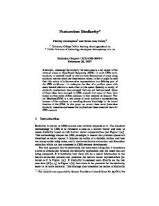
To visually explore the 7,344 equal-error rates that comprise the raw results of our experiment, we calculated the average equal-error rate across all subjects for each combination of the other five factors. These averages are presented across the 12 panels in Figure 1. Each panel contains three curves, depicting how the error rates of each of the three detectors changes with increased amounts of training. The strips above each panel explain what combination of factors produced the results in the panel. Updating is either None or Sliding Window; Feature Set is one of the combinations of hold times (H), keydown-keydown times (DD), keyup-keydown times (UD), and Return-key features (Ret); Impostor Practice is either None or Very High. Looking within any panel, we see that the error rates for all three detectors decrease as training increases. In particular, the Nearest Neighbor (Mahalanobis) error is much higher with only 5 repetitions, but improves and is competitive with the others with 100–200 repetitions. With few training repetitions, a practitioner might want to use either the Manhattan (scaled) or Outlier-score (z-count) detector. If we look beyond the individual panels to the four quadrants, the three panels in a quadrant correspond to the use of the three different feature sets. The curves in the three panels in each quadrant look nearly identical. It would appear that, so long as hold times and one of keydown-keydown or keyup-keydown times are used, the particular combination does not matter. The six panels on the left correspond to unpracticed-impostor error rates, and the six on the right correspond to very-practiced-impostor error rates. The curves in the right-hand panels are slightly higher. Consequently, impostor practice may represent a minor threat to the accuracy of keystroke-dynamics detectors. Finally, the six panels on the top correspond to non-updating detectors and the six on the bottom correspond to a sliding-window updating strategy. In particular, at 5 and 50 repetitions, the error-rate curves are much lower in the lower panels. An updating strategy seems to improve performance, especially if operating with only a few training repetitions. Overall, the lowest average equal-error rate was 7.1%, observed for the Manhattan (scaled) detector with 100 repetitions of training, hold and keydownkeydown features, sliding-window updating, and unpracticed impostors. Among
Why Did My Detector Do That?!
263
Detectors Nearest Neighbor (Mahalanobis) Outlier Count (z−score) Manhattan (scaled) 0 Updating : None Feature Set : H+UD Impostor Practice : None
50
100
150
200
Updating : None Feature Set : H+UD Impostor Practice : Very High 0.30 0.20 0.10
Updating : None Feature Set : H+DD Impostor Practice : None
Updating : None Feature Set : H+DD Impostor Practice : Very High
Updating : None Feature Set : H+DD+UD+Ret Impostor Practice : None
Updating : None Feature Set : H+DD+UD+Ret Impostor Practice : Very High
Equal−Error Rate
0.30 0.20 0.10
0.30 0.20 0.10 Updating : Sliding Window Feature Set : H+UD Impostor Practice : None
Updating : Sliding Window Feature Set : H+UD Impostor Practice : Very High
Updating : Sliding Window Feature Set : H+DD Impostor Practice : None
Updating : Sliding Window Feature Set : H+DD Impostor Practice : Very High
0.30 0.20 0.10
0.30 0.20 0.10 Updating : Sliding Window Feature Set : H+DD+UD+Ret Impostor Practice : None
Updating : Sliding Window Feature Set : H+DD+UD+Ret Impostor Practice : Very High
0.30 0.20 0.10 0
50
100
150
200
Number of Training Repetitions
Fig. 1. The average equal-error rates for each detector in the experiment as a function of training amount, feature set, updating strategy, and impostor practice. Each curve shows the effect of training on one of the three detectors. Each panel displays the results for one combination of updating (None/Sliding Window), feature set (H:hold times, DD:keydown-keydown times, UD:keyup-keydown times, Ret:Return-key times), and impostor practice (None/Very High). Comparisons can be made across panels because the scales are the same. For instance, the error-rate curves in the upper six panels (no updating) are higher than the curves in the lower six panels (sliding-window updating). This comparison suggests updating reduces error rates.
264
K. Killourhy and R. Maxion
the very-practiced impostor results, the lowest average equal-error rate was 9.7%, observed for the same combination of algorithm, training amount, feature set, and updating. The empirical results would seem to recommend this combination of detector, training amount, and feature set, but we would withhold a recommendation without further statistical analysis.
4
Statistical Analysis
The empirical results and visualization in Section 3 provide some insight into what factors might be important, but to make predictions about an anomaly detector’s future performance we need a statistical model. In this section, we describe the statistical analysis that we performed, and we present the model that it produced. 4.1
Procedure
The analysis is described in stages. First, we explain what a linear mixed-effects model is. Then, we describe how we estimate the model parameters. Finally, we lay out the procedure for selecting a particular linear mixed-effects model. Linear mixed-effects models. In statistical language, we intend to model the effect of six factors—algorithm, training amount, feature set, updating strategy, impostor practice, and typist (or subject)—on a response variable: the detector’s equal-error rate. Fixed and random are terms used by statisticians to describe two different kinds of effect. When a model has both fixed and random effects, it is called a mixed-effects model. The difference between fixed and random effects is sometimes subtle, but the following rule of thumb is typically applied. If we care about the effect of each value of a factor, the factor is a fixed effect. If we only care about the variation among the values of a factor, the factor is a random effect. For instance, we treat the algorithm as a fixed effect and the subject (or typist) as a random effect. Practitioners want to know which algorithm’s equalerror rate is lower: Manhattan (scaled) or Nearest Neighbor (Mahalanobis). We care about the effect of each value of the factor, so algorithm is a fixed effect. In contrast, practitioners do not want to know which subject’s equal-error rate is lower: Subject 1 or Subject 2. Neither subject will be a typist on their system. What we care about is how much variation there is between typists, and so the subject is a random effect. The following example of a mixed-effects model for keystroke-dynamics data may further elucidate the difference: Y = μ + Ah + Ti + Fj + Uk + Il + S + � S ∼ N (0, σs2 ) � ∼ N (0, σ�2 )
(1)
The notation in model equation (1) may seem daunting at first. On the first line of the model, Y is the response (i.e., the equal-error rate); μ is a baseline
Why Did My Detector Do That?!
265
equal-error rate; Ah , Ti , Fj , Uk , and Il are the fixed effects of the algorithm, training amount, feature set, updating strategy, and impostor practice, respectively; S is the random effect of the typist (or subject); and, � is the noise term. On the second line, the distribution of the random effect (S) is assumed to be Normal with zero mean and an unknown variance, denoted σs2 . On the third line, the distribution of the noise (�) is Normally distributed with zero mean and a different unknown variance, denoted σ�2 . The first term in the model equation (μ) denotes the average equal-error rate for one particular combination of fixed-effect factor values, called the baseline values. For instance, the baseline values might be the Manhattan (scaled) detector, 5 training repetitions, hold and keyup-keydown times, no updating, and unpracticed impostors. The average equal-error rate for that combination is μ (e.g., μ = 17.6%). For each of the five fixed effects, there is a separate term in the model equation (Ah , Ti , Fj , Uk , Il ). These terms denote the effect on the equal-error rate of departing from the baseline values. For instance, Ah is a placeholder for either of two departures from the Manhattan (scaled) baseline algorithm : A1 denotes the change to Outlier-count (z-score) and A2 denotes the change to Nearest Neighbor (Mahalanobis) detector. If the detector in the baseline combination were replaced with the Outlier-count (z-score) detector, the equal-error rate would be calculated as μ + A1 (e.g., 17.6% + 2.7 = 20.3%). For the random effect, there is both a term in the model equation (S) and a distributional assumption (S ∼ N (0, σs2 )). Like the fixed-effects terms, S represents the effect of a departure. Specifically, it introduces a per-subject effect that is negative (S < 0) for easy-to-discriminate subjects and positive (S > 0) for hard-to-discriminate subjects. Unlike the fixed-effects term, S is a random variable centered at zero. Its variance (σs2 ) expresses a measure of the typist-to-typist variation in the model. The final term in the model equation (�) is the noise term representing the unknown influences of additional factors on the equal-error rate. Like the random effect (S), � is a Normally distributed random variable. Its variance, σ�2 expresses a measure of the residual uncertainty in our equal-error predictions. Parameter estimation. When fitting a linear mixed-effects model, the unknown parameters (e.g., μ, Ah , Ti , Fj , Uk , Il , σs2 , and σ�2 ) are estimated from the data. There are a variety of accepted parameter-estimation methods; a popular one is the method of maximum-likelihood. From any estimate of the parameters, it is possible to derive a probability density function. Among all estimates, the maximum-likelihood estimates are those which give the greatest probability density to the observed data [18]. However, the maximum-likelihood methods have been shown to produce biased estimates of the variance parameters (e.g., σs2 ). The favored method is a slight elaboration called REML estimation (for restricted or residual maximum likelihood) which corrects for the bias in maximum-likelihood estimation [16,18]. We adopt the REML estimates.
266
K. Killourhy and R. Maxion
Model selection. In the discussion so far, we have explained how to interpret model equation (1) and how to do parameter estimation given such an equation. We have not explained how to select that model equation in the first place. For instance, consider the following alternative: Y = μ + Ah + Ti + AThi + S + � S ∼ N (0, σs2 ) � ∼ N (0, σ�2 )
(2)
In model equation (2), the terms corresponding to feature set (Fj ), updating (Uk ), and impostor practice (Il ) do not appear, so they are assumed to have no effect. An interaction term between algorithm and training (AThi ) appears, so the effect of training is assumed to depend on the algorithm. The interaction term denotes the effect on the equal-error rate of a departure from the baseline values in both algorithm and training amount. Without an interaction term, the effect would be additive (Ah + Ti ). With an interaction term, the additive effect can be adjusted (Ah +Ti +AThi ), increased or decreased as fits the data. Interaction effects can be estimated with REML estimation just like the other parameters. Looking at the relationship between the algorithm and training in Figure 1, we would expect to see a model with an AThi interaction. The Nearest Neighbor (Mahalanobis) has a much steeper slope from 5–50 training repetitions than the other two detectors. If the effects of the algorithm and training were additive (i.e., no interaction effect), the slopes of the three curves would be parallel. Consequently, model equation (2) might describe our data better. Model equations (1) and (2) are but two members of a whole family of possible models that we might use to describe our data. We need a method to search through this family of models and find the one that is most appropriate. Specifically, we need a way to compare two models and decide which one better explains the data. Of the various model-comparison strategies, one often employed is Schwartz’s Bayesian Information Criterion (BIC). The details are beyond the scope of this paper, but in brief a model’s BIC score is a summary combining both how well the model fits the data (i.e., the likelihood of the model) and also the number of parameters used to obtain the fit (i.e., the number of terms in the model). Having more parameters leads to a better fitting model, and having fewer parameters leads to a simpler model. BIC captures the trade-off between fit and simplicity. When comparing two models, we calculate and compare their BIC scores. Of the two, we adopt the one with the lower score [9]. Let us note one procedural issue when performing BIC-based model selection using mixed-effects models. REML estimation is incompatible with this heuristic, and so when comparing two models using BIC, the maximum-likelihood estimates are used. Once a model is selected, the parameters are re-estimated using REML. Intuitively, we use the maximum-likelihood estimates because, despite their bias, they allow us to do model selection. Then, once we have chosen a model, we can switch to the better REML estimates.
Why Did My Detector Do That?!
267
For the analysis of our experimental results, we begin with a model containing all the fixed effects, all interactions between those effects, and no per-subject random effect. We estimate the parameters of the model using maximum likelihood. Then, we add a per-subject random effect, estimate the parameters of the new model, and compare the BIC scores of the two. If the one with the per-subject random effect has a lower BIC (and it does), we adopt it. Then, in a stepwise fashion, we omit each term in the model, re-estimate the parameters, and recalculate the BIC. If we obtain a lower BIC by omitting any of the terms of the model, we drop the term which lowers the BIC the most and repeat the process. When no more terms can be dropped in this way, we adopt the current model as final and estimate the parameters using REML. This procedure is quite typical for mixed-effects model selection [7,16]. As another procedural note, we do not drop terms if they are involved in higher-order interactions that are still part of the model. For instance, we would not drop feature set (Fj ) as a factor if the interaction between algorithm and feature set (AFhj ) is still in the model. This so-called principle of hierarchy enables us to more easily interpret the resulting model [7]. For the statistical analysis, we used the R statistical programming language (version 2.10.0) [17]. To fit linear mixed-effects models, we used the lme4 mixed-effects modeling package (version 0.999375-32) [3]. 4.2
Results
We begin by describing the equation obtained through model selection since it informs us of the broad relationships between the factors. Then, we present the parameter estimates which quantify the effects of each factor and enable us to make predictions about a detector’s future error rates. Selected model. We arrived at the following model equation to describe the experimental data: Y = μ + Ah + Ti + Uk + Il + AT hi + AU hk + T U ik + U I kl + AT U hik + S+� S ∼ N (0, σs2 ) � ∼ N (0, σ�2 )
(3)
The equation has been split over multiple lines to make it easier to describe. The first line shows the main effects in the model. Note that the algorithm (Ah ), training amount (Ti ), updating (Uk ), and impostor practice (Il ) are all terms retained in the model, but the feature set (Fj ) has been dropped. During model selection, it did not substantially improve the fit of the model. This result is not surprising given how little change there was in any single quadrant of Figure 1. The second line shows the two-way and three-way interaction effects in the model. The interactions between the algorithm, training, and updating (AThi , AUhk , T U ik , and AT Uhik ) suggest a complex relationship between these three
268
K. Killourhy and R. Maxion
factors. The two-way interaction between updating and impostor practice (U Ikl ) suggests that updating may mitigate the impostor-practice threat. We will explore the nature of these interactions in greater detail when we look at the parameter estimates. The third line of model equation (3) includes a per-subject random-effect (S) along with the residual error term (�). From the presence of this per-subject term in the model, we conclude that there is substantial typist-to-typist variation. Some typists are easier to distinguish from impostors than others. Parameter estimates. Table 1 compiles the REML estimates of the parameters. Part (a) provides estimates of all the fixed effects, while Part (b) provides estimates of the random effects. The table is admittedly complex, but we include it for completeness. It contains all the information necessary to make predictions and to approximate the uncertainty of those predictions. In Part (a), row 1 is the estimate of μ, the equal-error rate for the baseline combination of factor values. The estimate, 17.6%, is the equal-error rate we would predict when operating the Manhattan (scaled) detector with 5 repetitions of training, no updating, and unpracticed impostors. Rows 2–26 describe how our prediction should change when we depart from the baseline factor values. Each row lists one or more departures along with the estimated change in the predicted equal-error rate. To predict the effect of a change from the baseline values to new values, one would first identify every row in which the new values are listed. Then, one would add the change estimates from each of those rows to the baseline to get a new predicted equalerror rate. For example, we can predict the equal-error rate for the Nearest Neighbor (Mahalanobis) detector with 200 training repetitions, no updating, and unpracticed impostors. The detector and training amount depart from the baseline configuration. Row 3 lists the effect of switching to Nearest Neighbor (Mahalanobis) as +19.2. Row 6 lists the effect of increasing to 200 training repetitions as −7.2. Row 15 lists the effect of doing both as −18.8 (i.e., an interaction effect). Since the baseline equal-error rate is 17.6%, we would predict the equal-error rate of this new setup to be 10.8% (17.6 + 19.2 − 7.2 − 18.8). As another example, we can quantify the effect of impostor practice. If no updating strategy is used, according to row 8, impostor practice is predicted to add +1.1 percentage points to a detector’s equal-error rate. If a sliding-window updating strategy is used, according to rows 7, 8, and 20, impostor practice is predicted to add +0.7 percentage points (−2.2 + 1.1 + 1.8). Consequently, impostor practice only increases an impostor’s chance of success by a percentage point, and the risk is somewhat mitigated by updating. While the aim of the statistical analysis is to predict what effect each factor has, it would be natural for a practitioner to use these predictions to choose the combination of factor values that give the lowest error. A systematic search of Table 1(a) reveals the lowest predicted equal-error rate to be 7.2%, using the Manhattan (scaled) detector with 100 training repetitions, sliding-window updating, and unpracticed impostors. For very-practiced impostors, the lowest
Why Did My Detector Do That?!
269
Table 1. Estimated values for all of the parameters in the model. The estimates are all in percentage points. Part (a) presents the fixed-effects estimates. The first row lists the combination of factor values which comprise the baseline along with the predicted equal-error rate. The remaining 25 rows list changes to the algorithm, amount of training, updating, and impostor practice, along with the predicted change to the equal-error rate. Part (b) presents the estimated typist-to-typist variation and the residual error. Both estimates are expressed as standard deviations rather than variances (i.e., by taking the square-root of the variance estimates) to make them easier to interpret. This table enables us to predict the error rates of a detector under different operating conditions, and also to estimate the uncertainty of those predictions.
1 2 3 4 5 6 7 8 9 10 11 12 13 14 15 16 17 18 19 20 21 22 23 24 25 26
μ Ah Ti Uk Il AThi
AUhk T Uik U Ikl AT Uhik
Algorithm Training Updating Impostor Estimates Manhattan (scaled) 5 reps None None 17.6 Outlier-count (z-score) +2.7 Nearest-neighbor (Mahalanobis) +19.2 50 reps −4.9 100 reps −6.9 200 reps −7.2 Sliding −2.2 Very High +1.1 Outlier-count (z-score) 50 reps −1.7 Nearest-neighbor (Mahalanobis) 50 reps −17.0 Outlier-count (z-score) 100 reps −1.3 Nearest-neighbor (Mahalanobis) 100 reps −17.9 Outlier-count (z-score) 200 reps −1.2 Nearest-neighbor (Mahalanobis) 200 reps −18.8 Outlier-count (z-score) Sliding −3.7 Nearest-neighbor (Mahalanobis) Sliding −7.7 50 reps Sliding −0.8 100 reps Sliding −1.3 200 reps Sliding +0.3 Sliding Very High +1.8 Outlier-count (z-score) 50 reps Sliding +2.3 Nearest-neighbor (Mahalanobis) 50 reps Sliding +8.1 Outlier-count (z-score) 100 reps Sliding +4.0 Nearest-neighbor (Mahalanobis) 100 reps Sliding +7.9 Outlier-count (z-score) 200 reps Sliding +3.0 Nearest-neighbor (Mahalanobis) 200 reps Sliding +8.4
(a): Estimates of the fixed-effects parameters of the model (in percentage points).
σs (Typist-to-typist) σ� (Residual)
Estimates of Standard Deviation 6.0 6.6
(b): Estimates of the random-effects parameters (as standard deviations).
270
K. Killourhy and R. Maxion
predicted equal-error rate is 10.1% for the same detector, training amount, and updating strategy. In Part (b) of Table 1, the typist-to-typist standard deviation (σs ) is estimated to be 6.0. Since the model assumes the typist-to-typist effect to be Normally distributed, we would predict that about 95% of typists’ average equal-error rates will lie withing 2 standard deviations of the values predicted from Part (a). For instance, suppose a new typist were added to a system operating with the baseline factor values. The overall average equal-error rate is predicted to be 17.6%, and with 95% confidence, we would predict that the average equal-error rate for the new typist will be between 5.6% and 29.6% (i.e., 17.6 ± 2 × 6.0). Likewise, there will be some day-to-day variation in a detector’s performance due to unidentified sources of variation. Table 1(b) provides an estimate of 6.6 percentage points for this residual standard deviation (σ� ). Calculations similar to those with the typist-to-typist standard deviation can be used to bound the day-to-day change in detector performance. Note that these confidence intervals are quite large compared to the fixed effects in Part (a). Future research might try to identify the source of the uncertainty and what makes a typist easy or hard to distinguish. A reader might ask what has really been learned from this statistical analysis. Based on the empirical results in Section 3, it seemed that the Manhattan (scaled) detector with 100 training repetitions and updating had the lowest error. It seemed that the feature set did not matter, and that impostor practice had only a minor effect. To answer, we would say that the statistical analysis has not only supported these observations but explained and enriched them. We now know which factors and interactions are responsible for the low error rate, and we can predict how much that low error rate will change as the typists change and the days progress.
5
Validation
The predictions in the previous section depend on the validity of the model. While the model assumptions can be checked using additional statistical analysis (e.g., residual plots to check Normality), the true test of a model’s predictive validity is whether its predictions are accurate. In this section, we describe such a test of validity and the outcome. 5.1
Procedure
We began by replicating the data-collection effort that was used to collect the data described in Section 3. The same apparatus was used to prompt subjects to type the password (.tie5Roanl) and to monitor their keystrokes for typing errors. The same high-precision timing device was used to ensure that the keystroke timestamps were collected accurately. From among the faculty, staff, and students of our university, 15 new subjects were recruited. As before, these subjects typed the password 400 times over 8
Why Did My Detector Do That?!
271
sessions of 50 repetitions each. Each session occurred on separate days to capture the natural day-to-day variation in typing rhythms. Their keystroke timestamps were recorded and converted to password-timing vectors, comprised of 11 hold times, 10 keydown-keydown times, and 10 keyup-keydown times. The evaluation procedure described in Section 3 was replicated using this new data set, for each algorithm, each amount of training data, each feature set, and so on. Each subject was designated as the genuine user in separate evaluations, with the other 14 subjects acting as impostors. We obtained 2,160 (3 × 4 × 3 × 2 × 2 × 15) new empirical equal-error rates from these evaluations. To claim that our model is a useful predictor of detector error rates, two properties should hold. First, the difference between the predicted equal-error rate and each subject’s average equal-error rate should be Normally distributed with zero mean and variance predicted by the model (σs2 ). A zero mean indicates that the predicted equal-error rates are correct on average. A Normal distribution of the points around that mean confirms that the typist-to-typist variability has been accurately captured by the model. Second, the residual errors, after the persubject effects have been taken into account, should also be Normally distributed with zero mean and variance predicted by the model (σ�2 ). This property confirms that the residual variability has also been captured by the model. To test these properties, we calculate the difference between each empirical equal-error rate and the predicted equal-error rate from the model. This calculation produces 2,160 prediction errors, 144 for each user. The per-typist effect for each user is calculated as the average of these 144 errors. The residual errors are calculated by subtracting the per-typist effect from each prediction error. 5.2
Results
4
Density
4 3
0
0
1
2
2
Density
5
6
6
8
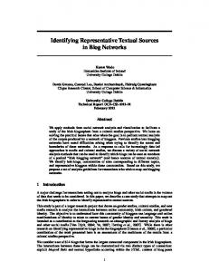
Figure 2 contains two panels, the left one showing the distribution of the pertypist effects, and the right one showing the distribution of the residual errors.
−0.10
−0.05
0.00
0.05
0.10
Per−Typist Effects ( n = 15 )
0.15
−0.2 −0.1
0.0
0.1
0.2
0.3
0.4
Residuals ( n = 2160 )
Fig. 2. The distribution of the per-typist effects and the residual errors compared to their predicted Normal distributions. The histogram on the left shows the per-typist effect for the 15 subjects. The histogram on the right depicts the residual errors. Both histograms closely match the Normal distributions predicted by the model. The match between the predicted and the observed distributions validates the model.
272
K. Killourhy and R. Maxion
Overlaid on each histogram is the Normal distribution predicted by the model. Both the per-typist-effects histogram and the residual-error histogram closely match the predicted Normal distributions. It is difficult to ascertain Normality from only 15 observations (one per subject), but the per-typist effects appear to be clustered around a mean of zero with the predicted variation about the mean. The residuals appear to be distributed as a bell-shaped curve with a mean of zero and the predicted variance. The tails of the distribution are slightly thicker than Normal, but the overall fit is still very close. Based on these graphs, we conclude that the model can accurately predict the detectors’ error rates on a new data set.
6
Related Work
Having demonstrated that we can explain detector’s error rates using influential factors from the evaluation, we should put our findings in the context of other keystroke-dynamics research. We cannot review the entire 30 year history of keystroke dynamics, but Peacock et al. [14] provide a concise summary of many of the developments during that time. In this section, we compare our findings to prior research into the influences of the same six factors. 1. Algorithm: Several researchers have compared different classification algorithms on a single data set, but few have compared anomaly detectors in this way. Cho et al. [5] compared the Nearest Neighbor (Mahalanobis) detector to an auto-associative neural network. Haider et al. [8] evaluated an Outlier-count (z-score) detector, a different neural network, and a fuzzy-logic detector. In earlier work, we tried to reimplement 14 detectors and replicate the results of earlier evaluations [12]. Our results differed wildly from the earlier ones (e.g., 85.9% vs. 1% error). In fact, the validation we report in Section 5 is one of the few successful replications of error rates from an earlier study using new data. 2. Amount of training: Joyce and Gupta [10] used only 8 password repetitions to train their detector, but they found that the same accuracy was observed with as few as 6 repetitions. Ara´ ujo et al. [1] considered training sets ranging from 6 to 10 repetitions. To our knowledge, while other researchers have published evaluations using as many as 200 training repetitions [5], no prior work has examined the error rates of detectors trained from as few as 5 to as many as 200 repetitions. In addition, earlier researchers have considered the effect of training on a single algorithm. We found that the effect of training cannot be separated from the effect of the algorithm. 3. Feature set: Ara´ ujo et al. [1] ran evaluations of a Manhattan (scaled) detector with seven different feature sets, including the three we used. They found that using all three types of feature (e.g., hold times, keydown-keydown times, and keyup-keydown times) produced the best results. In contrast, we found that, so long as hold times and either keydown-keydown times or keyupkeydown times are included, the particular combination has negligible effect.
Why Did My Detector Do That?!
273
Our findings benefit from the statistical analysis we used to check whether small effects are substantial enough to be included in the model. 4. Updating strategy: Ara´ ujo et al. [1] also compared a Manhattan (scaled) detector using updating to one with no updating. Kang et al. [11] compared a k-means detector trained with no updating to ones trained with growing and sliding windows. Both sets of researchers found that an updating strategy lowered error rates. Their results for individual detectors, coupled with our results for three detectors (backed by a validated statistical model), strongly support the claim that updating reduces detector error rates. Our results further demonstrate that window size (i.e., training amount) has an important effect on the error rate of a sliding-window detector. 5. Impostor practice: Lee and Cho [13] gave their impostors the opportunity to practice, but they did not describe how many repetitions of practice were taken by each impostor. Ara´ ujo et al. [1] split their impostor subjects into two groups. One group observed the genuine user typing the password, and one group did not. The observers seemed to be more successful at mimicking the typing style of the genuine user, but no statistical test was performed. In contrast, our work operationalized practice in terms of the number of repetitions and then quantified the effect of practice on error rates. 6. Typist-to-typist variation: To our knowledge, no prior work has substantially investigated whether some typists are easier to distinguish than others (i.e., the typist’s effect on detector error rates). Cho et al. [5] implicitly assumed a per-typist effect when they conducted a paired t-test in comparing two detectors. Often, standard deviations are reported along with error rates, but the current work may be the first to explicitly try to understand and quantify the substantial typist-to-typist effect. Based on our review of the related work, we can make two observations. First, even among those studies that have tried to explain the effects of various factors on detector error rates, interaction effects have not been considered. The present work reveals several complex interactions between algorithm, training, updating, and impostor practice. In the future, we should bear in mind the possibility of interactions between influential factors. Second, there have been few attempts to generalize from empirical results using statistical analysis. Some researchers have used hypothesis testing (e.g., t-tests) to establish whether there is a statistically significant difference between two sets of error rates [2,5], but such analysis is the rare exception rather than the rule. The current work demonstrates the additional insight and predictive capability that can be gained through statistical analysis. These insights and predictions would be missing if only the raw, empirical error rates were reported.
7
Discussion and Future Work
We initiated the current work to try to explain why different researchers, using the same detectors, were getting wildly different evaluation results. This work has shown that it is possible to replicate earlier results, but great care was taken
274
K. Killourhy and R. Maxion
to make sure that the details of the replication matched those of the original. We recruited new subjects, but tightly controlled many other factors of the evaluation (e.g., the password, keyboard, and timing mechanism). Showing that results can be replicated is a critical but often under-appreciated part of any scientific discipline. Fortunately, having succeeded, we can begin to vary some of these tightly controlled factors (using the very methodology proposed in this paper), and we can identify which ones threaten replication. The statistical model presented in this paper is certainly not the last word on which factors influence keystroke-dynamics anomaly detectors. There are factors we did not consider (e.g., the password), and for factors we did consider, there are values we did not (e.g., other anomaly detectors). For the factors and values we did investigate, the rigor of our methodology enables us to make claims with comparatively high confidence. Even knowing that our model is incomplete, and possibly wrong in some respects, it represents a useful guideline which future work can use, test, and refine.1 This work is exceptional, as explained in Section 6, for its statistical analysis and validation. Although many anomaly detectors are built upon statistical machine-learning algorithms, statistical analysis is rarely used in the evaluations of those detectors. Often a research paper will propose a new anomaly-detection technique and report the results of a preliminary evaluation. Such evaluations typically show a technique’s promise, but rarely provide conclusive evidence of it. As Peisert and Bishop [15] have advocated, researchers must follow preliminary, exploratory evaluations with more rigorous experiments that adhere to the scientific method. Our methodology offers a clear procedure for conducting more rigorous anomaly-detection experiments. We hope it is useful to other researchers.
8
Conclusion
In this work, we aimed to answer two questions. First, what influence do each of six factors—algorithm, training amount, feature set, updating, impostor practice, and typist-to-typist variation—have on keystroke-dynamics error rates? Second, what methodology should we use to establish the effects of these various factors? In answer to the first question, the detection algorithm, training amount, and updating were found to strongly influence the error rates. We found no difference among our three feature sets, and impostor practice had only a minor effect. Typist-to-typist differences were found to introduce substantial variation; some subjects were much easier to distinguish than others. In answer to the second question, we proposed a methodology rooted in the scientific method: experimentation, statistical analysis, and validation. This methodology produced a useful, predictive, explanatory model of anomaly-detector error rates. Consequently, we believe that the proposed methodology would add valuable predictive and explanatory power to future anomaly-detection studies. 1
As George Box notes, “All models are wrong, but some models are useful” [4].
Why Did My Detector Do That?!
275
Acknowledgments The authors are indebted to Howard Seltman and David Banks for sharing their statistical expertise, and to Patricia Loring for running the experiments that provided the data for this paper. We are grateful both to Shing-hon Lau for his helpful comments and also to the anonymous reviewers for theirs. This work was supported by National Science Foundation grant number CNS0716677, and by CyLab at Carnegie Mellon under grants DAAD19-02-1-0389 and W911NF-09-1-0273 from the Army Research Office.
References 1. Ara´ ujo, L.C.F., Sucupira, L.H.R., Liz´ arraga, M.G., Ling, L.L., Yabu-uti, J.B.T.: User authentication through typing biometrics features. IEEE Transactions on Signal Processing 53(2), 851–855 (2005) 2. Bartlow, N., Cukic, B.: Evaluating the reliability of credential hardening through keystroke dynamics. In: Proceedings of the 17th International Symposium on Software Reliability Engineering (ISSRE 2006), pp. 117–126. IEEE Press, Los Alamitos (2006) 3. Bates, D.: Fitting linear mixed models in R. R. News 5(1), 27–30 (2005) 4. Box, G.E.P., Hunter, J.S., Hunter, W.G.: Statistics for Experimenters: Design, Innovation, and Discovery, 2nd edn. Wiley, New York (2005) 5. Cho, S., Han, C., Han, D.H., Kim, H.I.: Web-based keystroke dynamics identity verification using neural network. Journal of Organizational Computing and Electronic Commerce 10(4), 295–307 (2000) 6. Denning, D.E.: An intrusion-detection model. IEEE Transactions on Software Engineering 13(2) (1987) 7. Faraway, J.J.: Extending Linear Models with R: Generalized Linear, Mixed Effects and Nonparametric Regression Models. Chapman & Hall/CRC (2006) 8. Haider, S., Abbas, A., Zaidi, A.K.: A multi-technique approach for user identification through keystroke dynamics. In: IEEE International Conference on Systems, Man and Cybernetics, pp. 1336–1341 (2000) 9. Hastie, T., Tibshirani, R., Friedman, J.: The Elements of Statistical Learning: Data Mining, Inference, and Prediction. Springer Series in Statistics. Springer, New York (2001) 10. Joyce, R., Gupta, G.: Identity authentication based on keystroke latencies. Communications of the ACM 33(2), 168–176 (1990) 11. Kang, P., Hwang, S.-s., Cho, S.: Continual retraining of keystroke dynamics based authenticator. In: Lee, S.-W., Li, S.Z. (eds.) ICB 2007. LNCS, vol. 4642, pp. 1203– 1211. Springer, Heidelberg (2007) 12. Killourhy, K.S., Maxion, R.A.: Comparing anomaly detectors for keystroke dynamics. In: Proceedings of the 39th Annual International Conference on Dependable Systems and Networks (DSN 2009), June 29-July 2, pp. 125–134. IEEE Computer Society Press, Los Alamitos (2009) 13. Lee, H.j., Cho, S.: Retraining a keystroke dynamics-based authenticator with impostor patterns. Computers & Security 26(4), 300–310 (2007) 14. Peacock, A., Ke, X., Wilkerson, M.: Typing patterns: A key to user identification. IEEE Security and Privacy 2(5), 40–47 (2004)
276
K. Killourhy and R. Maxion
15. Peisert, S., Bishop, M.: How to design computer security experiments. In: Proceedings of the 5th World Conference on Information Security Education (WISE), pp. 141–148. Springer, New York (2007) 16. Pinheiro, J.C., Bates, D.M.: Mixed-effects Models in S and S-Plus. Statistics and Computing Series. Springer, New York (2000) 17. R Development Core Team: R: A Language and Environment for Statistical Computing. R Foundation for Statistical Computing, Vienna, Austria (2008), http://www.R-project.org 18. Searle, S.R., Casella, G., McCulloch, C.E.: Variance Components. John Wiley & Sons, Inc., Hoboken (2006) 19. Swets, J.A., Pickett, R.M.: Evaluation of Diagnostic Systems: Methods from Signal Detection Theory. Academic Press, New York (1982)