Energy and Power Engineering, 2013, 5, 435-441 doi:10.4236/epe.2013.54B084 Published Online July 2013 (http://www.scirp.org/journal/epe)
Wide-Area Delay-Dependent Adaptive Supervisory Control of Multi-machine Power System Based on Improve Free Weighting Matrix Approach* Ziyong Zhang1, Zhijian Hu1, Yukai Liu1, Yang Gao2, He Wang1, Jianglei Suo1 1
School of Electrical Engineering, Wuhan University, Wuhan, China. Jiangsu Suzhou Power Supply Company, STATE GRID Corporation of China, Suzhou, China Email:
[email protected]
2
Received January, 2013
ABSTRACT The paper demonstrates the possibility to enhance the damping of inter-area oscillations using Wide Area Measurement (WAM) based adaptive supervisory controller (ASC) which considers the wide-area signal transmission delays. The paper uses an LMI-based iterative nonlinear optimization algorithm to establish a method of designing state-feedback controllers for power systems with a time-varying delay. This method is based on the delay-dependent stabilization conditions obtained by the improved free weighting matrix (IFWM) approach. In the stabilization conditions, the upper bound of feedback signal’s transmission delays is taken into consideration. Combining theories of state feedback control and state observer, the ASC is designed and time-delay output feedback robust controller is realized for power system. The ASC uses the input information from Phase Measurement Units (PMUs) in the system and dispatches supplementary control signals to the available local controllers. The design of the ASC is explained in detail and its performance validated by time domain simulations on a New England test power system (NETPS). Keywords: Adaptive Supervisory Controller (ASC); Delay-dependent Damping Control; Power Oscillation; IFWM; LMI; Free Weighting Matrix Approach; Time-varying Delay; WAMS
1. Introduction WITH the deregulation of power systems, many tie lines between control areas are driven to operate near their maximum capacity, especially those serving heavy load centers. Stressed operating conditions can increase the inter-area oscillation between different control areas and can even break up the system. The incidents of system outage resulting from these oscillations are of growing concern. Over the past few decades, attention has been focused on designing controllers to dampen inter-area oscillations. The traditional method of damping inter-area oscillations is via the installation of power system stabilizers (PSS) which provide control action through the excitation control of generators[1]. Local PSSs are usually tuned based on several typical operating conditions of corresponding generators. z An inappropriate coordination among the local controllers may cause serious problems [2]. It has been suggested that centralized controllers using wide-area signals rely on the PMUs technology[3]. *
This work is supported by Special Scientific and Research Funds for Doctoral Speciality of Institution of Higher Learning(20110141110032) and the Fundamental Research Funds for the Central Universities(2012207020205).
Copyright © 2013 SciRes.
PMUs are used to capture the power system’s dynamic data (e.g., voltages, currents, angles and frequency.) through synchronized measurements enabled by the GPS satellites. It has been shown that by using the remote signals the controller can enhance the damping of inter area oscillations and improve the overall dynamic performance of the power system[4]. A new PSS using two signals, the first to dampen the local mode in the area and the second, global signal, to dampen inter-area modes, is proposed in [5]. Application of techniques for designing robust power system damping controllers has been reported in the literature [6-9]. The solution to the control design problem based on the method of Riccati equations usually produces a controller that suffers from pole-zero cancellations between the system plant and the controller [10]. The application of the linear matrix inequality (LMI) approach as an alternative for damping controller design for PSS has been reported in [11,12]. A mixed-sensitivity based LMI approach has been applied to inter-area damping control design in [6,9]. In [9], FACTs are employed to damp inter-area oscillations. However, the cost of FACTs devices is quite high so that it currently reEPE
Z. Y. ZHANG ET AL.
436
stricts their wide use in power systems. In the controller design, signal transmission delays should be considered [7,8]. The delays can typically be in the range of 0.3 - 1.0 second[8]. As the delays are comparable to the time period of some of the critical inter-area modes, it should be accounted for in the design stage to ensure satisfactory control action. In this paper, a wide-area adaptive supervisory controller (ASC) for robust stabilization of multi-machine power systems is proposed. Based on the IFWM approach and networked control system (NCS) theory [1316], the ASC is designed by delay-dependent stabilization condition. In the stabilization conditions, the upper bound of feedback signal’s transmission delays is taken into consideration. The controller uses the input information (e.g. frequency, active power) provided by conveniently located PMUs and dispatches control signals to available local controllers. A particular feature of this controller is that it operates in addition to existing conventional PSSs and provides appropriate supplementary control signals only if and when needed. The performance and robustness of the controller are validated on a 4-generator 2-area test system.
2. Strategy of Adaptive Supervisory Control A New England test power system (NETPS) is used as the example to analysis strategy of adaptive supervisory control. The model of the AVR with supplementary WAM signals is shown in Figure 1. In this figure, VASCi is the output signal of the ASC[17,18] which is added to the AVR of each generator together with the output signal of four generators’ local PSS. The structure of the ASC is shown in Figure 2.
recent data and discards old data. When old data arrive at the controller, they are treated as packed loss. Assumption 3 The actual input obtained in (1) with a zero-order hold is piecewise constant function. The control network itself induces transmission delays and dropped data that degrade the control performance of the NCSs-based power system. Based on these three assumptions, we can formulate a closed-loop power system with a memoryless state-feedback controller: x (t ) Ax(t ) + Bu (t ) = * * u (t )= Kx(t − τ k ), t ∈ {ik h + τ k } , k = 1, 2,...,
where h is the sampling period; k = 1, 2,3,... are the sequence numbers of the most recent data available to the controller, which are assumed not to change until new data arrive; ik is an integer denoting the sequence number of the sampling times of the sensor {i1 , i2 , i3 ,...} ⊆ {1, 2, 3,...} ; and τ k is the delay from the instant ik h , when a sensor node samples the sensor data from the plant, to the instant when the actuator transfers the data to the plant. Clearly, ∞k 1 [ik h + τ k , ik +1h + τ k +1 ) =[t0 , ∞ ) . = From Assumption 2, ik +1 > ik is always true. The number of data packets lost or discarded is ik +1 − ik − 1 . When {i1 , i2 , i3 ,...} = {1, 2, 3, ...} , no packets are dropped. I f ik +1= ik + 1 , then h + τ k +1 > τ k , wh ich inc lude VT
-
1 1 + sTR
+
VREF
+
1 + sTC 1 + sTB
Σ
1 + sT1 1 + sT2
sTw 1 + sTw
K pss
△ωi, △Pi (i=1,3,5,8)
ASC
3.1. Modeling of NCS-Based Power system with Network-Induced Delay Consider the following linear system: (1)
where x(t ) ∈ R n is the state vector; u (t ) ∈ R m is the controlled input vector; and A and B are constant matrices with appropriate dimensions. For convenience, we make the following assumptions [19]. Assumption 1 The NCS consists of a time-driven sensor, an event-driven controller, and an event-driven actuator, all of which are connected to a control network. The calculated delay is viewed as part of the network-induced delay between the controller and the actuator. Assumption 2 The controller always uses the most Copyright © 2013 SciRes.
GENi
Local PSS
1 + sT3 1 + sT4
VASCi
△ω i
EF
KA 1 + sTA
+ VPSSi
3. Controller Design Considering Signals Transmission Delay
= x (t ) Ax(t ) + Bu (t )
(2)
Global signals
Adaptive supervisory controller
Figure 1. The designed model of ith exciter using the WAMs signals. G1
△ω 1
VASC1
Area 1
△ω3
Adaptive Supervisory controller
△ω 8
G8
VASC8 VASC5
G3
VASC3
△ω5
Area 2
G5
Figure 2. The input and output signals of the adaptive supervisory controller.
τ k = τ 0 and τ k < h as special cases. So, system (2) represents an NCS-based power system and takes the EPE
Z. Y. ZHANG ET AL.
effects of both a network-induced delay and dropped data packets into account. Below, we assume that u (t ) = 0 before the first control signal reaches the plant, and that a constant η > 0 exists that
437
equations are true for any matrices N = N1T N 2T M = M 1T M 2T
T
s ,
(3) ik h 0 2ς T (t ) M x(ik h) − x(t − η ) − ∫t −η x ( s )d = Based on this inequality, we can rewrite NCS (2) as x (t )= Ax(t ) + BKx(ik h), t ∈ [ik h + τ k , ik +1h + τ k +1 ) , k = 1, 2, ... , φ (t ), x(t0 − η )e A(t −t0 +η ) = x(t ) =
(4)
X X any = matrix X 11 12 ≥ 0, the following equation * X 22 holds: t
∫t −η ς
T
t
(t ) X ς (t )ds − ∫t −η ς T (t ) X ς (t )ds t
φ
T
k
and
such that the following matrix in-
φ11 φ12 − M 1 η AT Z T T * φ22 − M 2 η K B Z < 0, * * −Q 0 * * − η Z *
X N = Ψ1 ≥ 0, * Z X M = Ψ2 ≥ 0, * Z
(11) In addition, the following equation is also true t
t
ik h
− ∫t −η x T ( s ) Zx ( s )ds = − ∫i h x T ( s ) Zx ( s )ds − ∫t −η x T ( s ) Zx ( s )ds k
(12) Calculating the derivative of V ( xt ) along the solutions of system (4) for t ∈ [ik h + τ k , ik +1h + τ k +1 ) , adding the right sides of (9)-(11) to it, and using (12) yield V ( xt ) 2 xT (t ) Px (t ) + xT (t )Qx(t ) − xT (t − η )Qx(t − η ) = + η x T (t ) Zx (t ) − ∫
t
x T (t ) Zx (t )ds
t −η
= 2 xT (t ) Px (t ) + xT (t )Qx(t ) − xT (t − η )Qx(t − η ) t
i h
ik h
t −η
k + η x T (t ) Zx (t ) − ∫ x T ( s ) Zx ( s )ds − ∫ x T ( s ) Zx ( s )ds
t + 2ς T (t ) N x(t ) − x(ik h) − ∫ x ( s )d s ik h
(5)
ik h + 2ς T (t ) M x(ik h) − x(t − η ) − ∫t −η x ( s )d s t
ik h
+ ης T (t ) X ς (t ) − ∫i h ς T (t ) X ς (t )d s− ∫t −η ς T (t ) X ς (t )d s k
(6)
ˆ (t ) − t ξ T (t , s )ψ ξ (t , s )d s = ξ1T (t )φξ 1 1 2 ∫i h 2 k
ik h
− ∫t −η ξ (t , s )ψ 2ξ 2 (t , s )d ,s
(7)
T 2
(13)
where
where
φ11 = PA + AT P + Q + N1 + N1T + η X 11 ,
φ11 + η AT ZA = * φˆ *
φ12= PBK − N1 + N + M 1 + η X 12 , T 2
φ13 = − N 2 − N + M 2 + M + η X 22 . T 2
ik h
= ης T (t ) X ς (t ) − ∫i h ς T (t ) X ς (t )d s− ∫t −η ς T (t ) X ς (t )d s
This section first present a new stability criterion for NCS (4), assuming the gain, K , is given. Theorem 1. Consider NCS (4), given a scalar η > 0 , the system is asymptotically stable if there exist matrices X X and X 11 12 ≥ 0 , and any P > 0, Q ≥ 0, Z > 0,= * X 13
M = M 1T M 2T equalities hold:
(10)
T
3.2. Delay-dependent Stability Analysis
N N = 1 N2
s ,
(9)
where ς (t ) = xT (t ), xT (ik h) . On the other hand, for
where the initial condition function, φ (t ) , of the system 0 is continuously differentiable and vector-valued. =
appropriately dimensioned matrices
and
with appropriate dimensions:
t = 0 2ς T (t ) N x(t ) − x(ik h) − ∫i h x ( s )d k
(ik +1 − ik )h + τ k +1 ≤ η , k = 1, 2, ...
T
T 2
φ12 + η AT ZBK φ22 + η K B ZBK T
T
*
− M1 − M2 , − Q
T Proof. Choose the Lyapunov-Krasovskii functional = ξ1 (t ) xT (t ), xT (ik h), xT (t − η ) , candidate to be:
t
= V ( xt ) xT (t ) Px(t ) + ∫t −η xT ( s )Qx( s )ds +∫
0
∫
t
−η t +θ
x T ( s ) Zx ( s )dsdθ ,
T
(8)
where P > 0, Q ≥ 0, and Z > 0 are to be determined. From the Newton-Leibnitz formula, the following Copyright © 2013 SciRes.
ξ 2 (t , s) = ς T (t ), x T ( s) .
Thus, if ψ i ≥ 0, i = 1, 2, and φˆ < 0 , which is equivalent to (5) by the Schur complement, then V ( xt ) < 2 −ε x(t ) for a sufficiently small ε > 0 , which guarantees that system (4) is asymptotically stable. This comEPE
Z. Y. ZHANG ET AL.
438
pletes the proof. When M = 0 and Q = ε I (where ε > 0 is a sufficiently small scalar), the following corollary readily follows from Theorem 1. Corollary 1 Consider NCS (4), given a scalar η > 0 , the system is asymptotically stable if there exist matrices X X and X 11 12 ≥ 0 , and any approP > 0, Z > 0, = * X 22 N priately dimensioned matrix N = 1 such that ma N2 trix inequality (6) and the following one hold: Ξ11 Ξ12 η AT Z (14) = Ξ * Ξ 22 η K T BT Z < 0, * −η Z * where Ξ11 = PA + AT P + N1 + N1T + η X 11 , Ξ12 = PBK − N1 + N 2T + η X 12 , Ξ 22 = − N 2 − N 2T + η X 22 .
3.3. Design of State Feedback Controller Theorem 1 is extended to the design of a stabilization controller with gain K for system (4). Theorem 2. Consider NCS (4), for a given scalar η > 0 , if there exist matrices L > 0, W ≥ 0, R > 0, and Y Y = Y 11 12 ≥ 0, and any appropriately dimensioned * Y22 T
T
matrices S = = S1T S2T , T T1T T2T , and V such that the following matrix inequalities hold: Ξ11 Ξ12 − T1 η LAT * Ξ 22 − T2 ηV T BT (15) Ξ < 0, * * −W 0 − η R * * * S Y = Π1 ≥ 0, −1 * LR L T Y = Π2 ≥ 0, −1 * LR L
(16) (17
where Ξ11 = AL + LAT + W + S1 + S1T + ηY11 , Ξ12 = BV − S1 + S2T + T1 + ηY12 , Ξ 22 = − S2 − S2T + T2 + T2T + ηY22 . then the system is asymptotically stable, and K = VL−1 is a stabilizing controller gain. Proof. Pre-and post-multiply φ in (5) by diag P −1 , P −1 , P −1 , Z −1 , and pre- and post-multiply
{
}
Copyright © 2013 SciRes.
ψ i , i = 1, 2, in (6) and (7) by diag { P −1 , P −1 , P −1} . Then, make the following changes to the variables: −1 −1 = L P= , R Z= , V KL,
= Si LN = LM = 1, 2, i L, Ti i L, i
{
}
{
}
= W LQL= , Y diag P −1 , P −1 ⋅ X ⋅ diag P −1 , P −1 .
These manipulations yield matrix inequalities (15)(17). This completes the proof. Note that the conditions in Theorem 2 are no longer LMI conditions due to the term LR −1 L in (16) and (17). Thus, that cannot use a convex optimization algorithm to obtain an appropriate gain matrix, K , for the statefeedback controller. This problem can be solved by using the idea for solving a cone complementarity problem [20]. Define a new variable, U, for which LR −1 L ≥ U ; and −1 let = P L= , H U −1 , and Z = R −1 . Now, we convert the nonconvex problem into the following LMI-based nonlinear minimization problem: Minimize Tr { LP + UH + RZ } Subject to (15) and Y S Y ≥ 0, * U * L I ≥ 0, U * * P
T H ≥ 0, U * I R ≥ 0, H *
P ≥ 0, Z I ≥ 0. Z
(18)
We use the ICCL algorithm to obtain ηmax and K optimal for power systems because of its advantages. Algorithm. Step1: Choose a sufficiently small initial η > 0 , such that there exists a feasible solution to (15) and (18). Set a specified number of iterations N. Step2:Find a feasible set of values satisfying (15) and (18), ( P0 , L0 , W , S , T , Y , Z 0 , R0 , U 0 , H 0 , V ) .Set k =0 Step3: Solve the following LMI problem for the variables P, L, W , S , T , Y , Z , R,U , H ,V , and K : Minimize Tr { LPk + Lk P + UH k + U k H + RZ k + Rk Z } Subject to (15) and (18). Set = Pk +1 P= , Lk +1 L= , U k +1 U = , H k +1 H= , Rk +1 R, and Z k +1 = Z . Step4: For the K obtained in step 3, if LMIs (15) and (18) are feasible for the variables P, Q, Z , N , M , and X , then set ηmax = η , increase η , and return to Step 2. If LMIs (5)-(7) are infeasible and without a specified number of iterations, then exit. Otherwise, set k= k + 1 and go to Step 3. Figure 3 shows the flowchart of nonlinear iterative optimization algorithm for the state feedback controller design. This condition and nonlinear iterative optimization algorithm, which has an improved stop condition, are used to design a state-feedback networked controller. But the operating state variables of wide-area power sysEPE
Z. Y. ZHANG ET AL.
tem cannot be completely observed, it is necessary to use measurable states. Here, combining theories of state feedback control and state observer, the ASC is designed and time-delay output feedback robust control is realized for power system[21].
4. Study System The New England test power system (NETPS) which consists of ten synchronous units in the system connected by weak tie-lines is shown in Figure 4[22]. This system is considered to be one of the benchmark models for performing studies on inter-area oscillations because of its realistic structure and availability of system parameters. To validate the designed robust controller, the following disturbances were considered: Case 1: A 2-phase fault at one of the lines between buses 6-11 followed by successful auto-reclosing of the circuit breaker after 4 cycles; Case 2: A 3-phase fault at one of the lines between buses 6-11 followed by successful auto-reclosing of the circuit breaker after 4 cycles;
439
5. Simulation Results To validate the performance and robustness of the proposed control scheme involving ASC, simulations were carried out corresponding to the probable fault scenarios in the test system. If no time delay was considered, the simulation results were given in [17,18]. In each of the two cases, the total time delay for the feedback signals to arrive at the controller, then for the controller to send the signals to AVRs is 0.5 seconds.
5.1. Case 1 The rotor speed difference responses of multi-machine power system following a 2-phase fault are shown in Figures 5 and 6.
5.2. Case 2 The rotor speed difference responses of multi-machine power system following a 3-phase fault are shown in Figures 7 and 8. 8
1
37
30
25
Input matrix A and B Set iteration nunber N and step ∆η Choose a small initial values η > 0
27
1
38 3
10
18
17
39
9
L25
L26
Find a feasible set of values stasfiying (15) and (18) : ( P0 , L0 , W , S , T , Y , Z 0 , R0 , U 0 , H 0 , V ) and then set k=0
21
16
15
Ld16 6
Ld15 4
Minimise Tr { LPk + Lk P + UH k + U k H + RZ k + Rk Z } Subject to (15) and (18) Set η k = η0
29
28
26
2
14
13
5
23
6
9
19
12 11
k= k + 1
36
24
22
20
7 10 8
Set= Pk +1 P= , Lk +1 L= , U k +1 U = , H k +1 H , = Rk +1 R= , and Z k +1 Z
32
31
Y
2
3
33
34 5
4
35 7
Figure 4. The New England test power system. Satisfy (15) and (18)?
k