Widely linear estimation with complex data - Signal ...

1BEiE

0‘ 10”

10“ lo-‘ False Alarm Probability

Fig. 3. ROC for standard and robust LRT with different contamination parameters.

TRANSACTIONS ON SIGN& PROCESSING, VOL. 43, NO. 8, AUGUST 1995

V. CONCLUSION This correspondence has described a procedure for testing which nonlinear dynamic model from a finite class generated a particular random process. The procedure uses extended Kalman filters (EKF’s) tuned to each admissible model, and constructs a robust likelihood ratio test (LRT) from the EKF prediction error sequences. When the E m s are operating in the linear region, the signal prediction errors closely approximate the innovations sequence for that signal. In particular, the prediction errors are very close to Gaussian and the LRT‘s, which are designed for Gaussian sequences, are well mqtched. However when the linearity approximation breaks down, the prediction errors depart from being Gaussian, and the LRT fails badly. To overcome this, the LlyT is robustified using a simple generalization of Huber’s method. The likelihood ratio is dynamically censored, with the censor points computed online from the EKF error covariance estimates. Simulations have illustrated that the method can perform very well in comparison with the standard approximate LRT. Factors that we have not addressed are: a) the prediction error may become colored, which could effect the robust LRT; b) the contamination parameters could be adaptively adjusted to take account of the extent of the linearization errors in the EKF, c) the effect of unknown initial conditions; and d) the issue of model mismatch. REFERENCES

3n

0.85

[l] A. S. Willsky, “A survey of design methods for failure detection in dynamic systems,” Automuticu, vol. 12, pp. 601-61 1, 1976. [2] M. Basseville and A. Benveniste, Eds., “Detection of abrupt changes in signals and dynamic systems,” Springer Lecture Notes in Control and Information Sciences, vol. 77, 1986. [3] B. D. 0.Anderson and J. B. Moore, Optimal Filtering. E n g l e w d Cliffs, NJ: Prentice-Hall, 1979. [4] P. J. Huber, “A robust version of the probability ratio test,” Ann. Math. Star., vol. 36, pp. 1753-1758, 1965. [5] L. B. White, “A robust LRT for testing between nonstationary nonlinear dynamic systems,” Defence Science and Technology Organization, Australia, Signal Analysis Discipline Report, SA/93/09U, 1993.

-

0

0.65

1o

1

.~

1o-2

10.’ False Alarm Probability

10”

Widely Linear Estimation with Complex Data

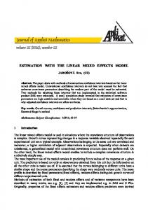
Fig. 4. ROC curve for FMPM example.

Bernard Picinbono and Pascal Chevalier common forms of angle modulated signals. The problem is to determine which of PM or FM is present on a particular signal. The PM model is

+ ut +

=

zt I Ho = cos [z!”] ut

(12)

I. INTRODUCTION Mean square estimation (MSE)is one of the most fundamental techniques of statistical signal processing. The basic problem can be

whilst the FM model is z;y1 = A s p

yt(yl= y p zt

+ fflt

+

1 Hi = cos [y,“’]

+ ut

Abstract-Mean square eStimntioa of complex and normal data is not linear as in the real case but widely linear. The purpose of this correspondence is to calculate the optimum widely linear mean square estimate and to present its main properties. The advantage with respect to linear procedure is espedplly analyzed.

(13)

where the noises are as above. Signals were generated with cf = 0 . 1 , ~ ~= : 0.01,PO = PI = 0.01, and the remaining parameters identical to the above. Fig. 4 shows the ROC curve. Again, a significant improvement is noted.

Manuscript received January 24, 1994; revised January 20, 1995. The associate editor coordinating the review of this paper and approving it for publication was Dr. Monique Fargues. B. Picinbono is with the Labomtoire des Signaux et Systhes, Su*lec, Gif SUI Yvette, France. P. Chevalier is with the Thomson-CSF, Division RGS, Gennevilliers, France. IEEE Log Number 9412636.

1053-587X/95$04.00 0 1995 IEEE

Authorized licensed use limited to: Bernard Picinbono. Downloaded on December 15, 2008 at 09:27 from IEEE Xplore. Restrictions apply.

IEEE TRANSACI'IONSON SIGNAL PROCESSING, VOL. 43, NO. 8. AUGUST 1595

stated as follows: Let y be a scalar random variable to be estimated (estimandum) in terms of an observation that is a random vector x. The estimate y that minimizes the MS error is then the regression or the conditional expectation value E[yIx].This result is usually given when x and y are real. However, it remains valid when these quantities are complex valued. If x and y are jointly normal with zero mean value and are real, then the regression is linear. However, this is no longer true for normal complex data, where the regression is linear both in x and x* and is called widely linear (WL). It is interesting to study the properties of WL systems for MSE without introducing the normal assumption. In LMSE, the problem is to find an estimate written as y

= hHx

(1.1)

where A means the complex conjugation and transposition (or Hermitian transposition). Because y is a scalar product, it results from the definition of such a product that y is a linear function of the vector x, as defined in classical linear algebra. Consider now the scalar y' defined by

Replacing y with (2.1) gives

where

I' = E [ x x H ] C ; =

r = E[y*x];s = E[yx].

(2.6)

From (2.4) and (2.5), we find the solutions expressed as U = [r - cr-'*~*]-'[r - cr-l*s*] v = [r' - C * ~ - ~ C ] --~c*r-'r]. [~*

(2:7) (2.8)

The corresponding mse is also deduced from the projection theorem, and by using (2.1), (2.4), and (2.5), we obtain E'

= E[~Y~'~ - (uHr

+vHg*).

(2.91

This error is smaller than &, which is the error that is obtained with a strictly LMSE-like (1.1) and equal to E[lyl'] - rHI'-'r. The advantage of the WLMSE procedure over the LMSE is characterized by the quantity 6 ~ ' = E: - E', which can be expressed as

6~= ' [s* - c*r-'rlH[r* -c*~-'c]-~ where X* is the complex conjugate of x, and g is another complex [a* ~*r-'r]. (2.10) vector. This is the general form of the regression for complex normal random variables. It is clear that y' is not a linear function of x. It is always nonnegative because the matrix [r*- c * ~ - ~ is c ] However, the moment of order k of y' is completely defined from positive definite, and consequently, 6s' = 0 only when s* the moments of order k of x and x*, which characterizes a form of c*r-'r = 0. linearity. This is why (1.2) will be called a wide sense linear filter At this step, it is worth pointing out that all the previous calcuor system. lations could be realized by using only real quantities. However, by The general purpose of this correspondenceis to show that taking doing so, the compact expression of the complex quantity j j is less into consideration WL systems defined by (1.2) instead of strictly obvious, and (2.10) takes a much more complex form. Furthermore, linear ones defined by (1.1) can yield significant improvements in the comparison with the strictly linear procedure characterized by estimation problems using complex data. This result can appear rather v = 0 is less obvious with real quantities than with (2.1). Finally, in natural and was indicated under restrictive conditions in [l] and [2], the strictly linear case, nobody has the idea to transform the complex and the principles of a more general presentation appear in [3, p. 4131 Wiener-Hopf equation r u = c in a set of two real equations. without the detailed analysis discussed hereafter. In reality, there is at least one reason why (1.2) is not widely used. This is due to the fact IU. EXAMPLES that in almost all calculations using complex Gaussian distribution, the assumption of circularity is explicitly (or implicitly) introduced (see [3, p. 1181). T h i s assumption is valid in many practical situations, A. Jointly Circular Case and in this case, the last term of (1.2) disappears in such a way This situation is characterized by that complex signals and systems can be treated as if they were c = 0;8 = 0. (3.1) real. However, this assumption, which is strongly connected with stationarity [4], has no reason for being general. This justifies the This assumption is well known in the normal case (see [3, p. 1181). analysis of this correspondence. In reality, it is sometimes used in the definition of complex normal random vectors, [5], [6, p. 1281, where the term "strongly normal" U. WL MEAN SQUARE ESTIMATION is used and is used in [7] as well. In particular, one can show that The problem of WL mean square estimation (WLMSE) is to find under some conditions, the Fourier components of stationary signals are complex circular random variables. The analytic signal of a real the vectors U and v in such a way that stationary signal is also second-order circular. The term of circularity y = UHX VHX* (2.1) comes from the fact that if (3.1) holds, the random vectors x and gives the minimum mse E[ly - Sl']. For this purpose, the first point x exp0'a) have the same second-order properties for any (Y.Note to note is that the set of scalar complex random variables .(U) in the that (3.1) characterizes only second-order circularity, and the concept form .(U) = aHx(W) bHx*(W),where a and b belong to C N must be extended when using higher order statistics. Note also that constitutes a linear space. It becomes a Hilbert subspace with the (3.1) means a joint circularity and is then an assumption on x and y. It immediately results from (2.8) that (3.1) implies v = 0. . a result f is the projection of y scalar product ( a , a ' ) = E ( Z * Z ' )As onto this subspace and is characterizedby the orthogonalityprinciple Similarly, (2.7) gives U = r-'r. Thus, the assumption of joint circularity implies that the WLMSE (2.1) takes the form (1.1) and (y - y) U x; (y - y) Y x*. (2.2) is strictly linear. It is also clear that (2.10) gives 6 ~ '= 0, and the conclusion is that in the case of a joint circularity, the strictly linear The symbol U means that all the componentsof x or x* are orthogsystem (1.1) is sufficient to reach the best performance. This is one onal to y - 6 with the previous scalar product. As a consequence, of the arguments justifying the interest of circularity. However, even these equations can be written in terms of expectations, which yields if circularity appears in many practical situations [7], there are cases E ( i * x ) = E ( y * x ) ;E ( $ * x * )= E ( y * x * ) . (2.3) where it cannot be introduced.

+

+

Authorized licensed use limited to: Bernard Picinbono. Downloaded on December 15, 2008 at 09:27 from IEEE Xplore. Restrictions apply.

JEEE TRANSACTIONS ON SIGNAL PROCTSING, VOL. 43, NO. 8, AUGUST 1995

2032

B. Circular Observation Suppose now that the second assumption (3.1) is deleted. This means that circularity is only valid for the observation and is chmcterized by C = 0, whereas no specific assumption is introduced for the estimandum y. In this case, (2.7) and (2.8) are greatly simplified and become

and h ( t )is determined by the otthogonality equation

1

h(8)yZ(7

Thus, a nonzero vector s necessarily implies an increment of the performance of estimation when using the structure (1.2) instead of (1.1). C. Case of a Real Estimandum y The estimation of a real quantity from complex data appears in many situations as, for example, when the observation comes from Fourier components of a real signal, some real parameters of which have to be estimated. Suppose then that y is real, x still being complex. This obviously implies that r = s in (2.6). It results from (2.7) and (2.8) that U = v*,and consequently, y = 2 Re (uHx).

(3.4)

(3.9)

where yZ(7) = E [ z ( t ) s * (t 7)] and yVZ(.) = E [ y ( t ) z * ( t T)]. A Fourier transformation yields the frequency response

JW his means that the term uHx in (2.1) is the same as the one obtained when using strictly linear estimation. This fact can be explained by noting that the circularity assumption implies that the vectors x and x* are uncorrelated. Thus, the Hilbert subspaces generated by x and x* are orthogonal, and taking into account x* does not change the term coming from x only. This also explains the simplification of (2.10) that becomes

- @).dB= rVz(7)

= [r,(v)]-lrYz(~)

(3.10)

where r,(w)is the power spectrum of z ( t ) , and r Y z ( v ) is the Fourier transform of yY (7). The mean square error is then

On the other hand, the WLMSE of

y ( t ) is, as in (3.6)

C W L ( t )= 2Yl ( t )

(3.12)

where y1 (t) is the real part of OL given by (3.8). However, as z ( t ) is circular, we have E[&(t)] = 0, and then

E h ~ ( t ) l ' l= E[y?(t)l+ E[Y;(~)]= 2E[y:(t)]

(3.13)

where yz(t) is the imaginary part of c ~ ( t )As . a result, we have E [ & L ( ~ ) ]= 2E[1c~(t)1~], and (3.11) becomes

This shows the advantage of the wide sense linear procedure over the strictly linear one. The conclusion is general: When the complex data are not jointly circular, the LMSE is not the best procedure of estimation that only uses second-order propedes of the signals.

Similarly, the estimation error takes the form E'

= E(y2)

- 2Re(uHr).

(3.5)

The main property of the estimate (3.4) is that it is real, although there is no reason for the strictly linear estimate to be real, which is not convenient when estimating a real quantity. The advantage of the structure (1-2) with respect to (1.1) is even more clear when the observation x is circular. In fact, as seen previously in Section ID-B, the vector U is the same as the one that must be used to realize the LMSE of y with (1.1). Thus, by using this vector, the two estimators (1.1) and (1.2) become

and the corresponding errors are

D. Singular Estimation The estimation is singular when the mse is zero. If the wide sense linear mean square error (2.9) is zero, the estimandum y belongs to the Hilbert subspace introduced after (2.1) and can then be written as

+

y = aHx bHx*.

(3.15)

It is now interesting to study the behavior of the strictly LMSE when (3.15) holds or in the case of singular wide sense LMSE. Note first that if b = 0, (3.15) becomes strictly linear. In this case, singular estimation appears equally well,with the two forms of linear procedures. Let us now investigate the complete opposite situation. It corresponds to the case where the strictly linear procedure provides a zero estimation. his means that the m e E; is equal to ~ [ l y l ' ] . This situation appears when r defined by (2.6) is zero, which means that the estimandum y and the observation x are uncorrelated. By replacing y given by (3.15) in (2.6), we obtain

Note that the quantity uHr is positive because it is equal to uHr u , and r is a positive definite matrix. In conclusion, the wide sense linear estimator (3.6) provides a real estimate and a decrease of the r=ra+Cb. (3.16) error that is twice as great as the strictly linear estimate, which in ' uHr. general is complex. It is also clear from (3.7) that 6 ~ = As I' is positive definite, the condition r = 0 is equivalent to These results can especially be applied in the classical nona = -I'-'Cb. (3.17) causal Wiener filtering. Let z ( t ) and y(t) be two jointly stationary continuous-timesignals. Supposefurther that y(t) is real and that z ( t ) Then, if C # 0 or if x is not circular, it is possible to associate is complex and second-order circular, which means that E [ z ( t ) z ( tto any nonzero vector b another n o m vector a given by (3.17) T ) ] = 0. This is, for example, the case of the analytical signal of a real stationary signal (see [4, p. 2301). The strictly linear estimate of and such that y given by (3.15) is uncorrelated with x. This implies a zero LMSE. On the other hand, because of (3.15), c given by (2.1) y(t) can be expressed as (see [4, p. 4501) is equal to y, and the m e is zero, which means singular estimation. We then have zero estimation with the strictly linear procedure and perfect estimation with the wide sense liiear procedure.

Authorized licensed use limited to: Bernard Picinbono. Downloaded on December 15, 2008 at 09:27 from IEEE Xplore. Restrictions apply.

~

W E TRANSACTIONS ON SIGNAL PROCESSING, VOL. 43, NO. 8, AUGUST 1995

IV. CONCLUSION We have presented a compact approach of the general problem of linear estimation with complex data. This problem is usually presented as a straightforward extension of the results obtained in the real case. By doing so, it is in general impossible to reach the optimum performance that can be deduced from the second-order statistics. This requires the introduction of widely linear systems. The structure of WLMSE has been determined. From this result, we have shown that widely linear systems can yield significant improvements in estimation performance with respect to strictly linear systems generally used, except when the circularity assumption is introduced. It is even possible to reach singular WL estimation while strictly linear systems give a zero estimation.

2033

(see [l, p. 133, Assumptions (1)-(3)1), the Fisher information matrix for N consecutive measurements is given by [ J ~ ( @ ) ] k ,= e

[mjlrk’(e)iT~~l(e)[m~)(8)i

+ str{ 1 RLN1(8)R~’(@)R,’(e)R~)(B)) (1)

where ”(8) = [m(O),m(l),.-.,m(N - 1)IT and R N ( ~ is) the N x N Toeplitz matrix of the covariances, that is, [ R N ( ~ )=] ~ , ~ T(P

- (I).

In [2], the following approximation is proposed for [ J ~ ( @ ) ] k , t

FUTERENCES

W. M. Brown and R. B. Crawe, “Conjugatelinear filtering,”IEEE Trans. Inform. Theory, vol. IT-15,pp. 462-465, 1969. W. A. Gardner, “Cyclic Wiener filtering: Theory and methods,” IEEE Trans. Cormrun., vol. 41, pp. 151-163, 1993. B. Picinbono, Random Signals und Systems. Englewood Cliffs, NJ Prentice-Hall, 1993. -, “On circul;lyity,” IEEE Trans. Signal Processing, vol. 42, pp. 3473-3482, 1994. K. Miller, Multidimensional Gaussian Distributions. New York Wiley, 1964. M. W v e , Probability Theory, vol. 2. New York Springer Verlag, 1978. S . Kay, Modem Spectral Analysis, Theory and Applications. Englewood Cliffs, NJ Prentice-Hall, 1988.

where: d ~ ( w , 8 is ) the discrete Fourier transform of the vector m ~ ,

that is N-1

dN(w,~) =

m(n)e-Jwn.

(3)

?I=O

Note that in [2, Eiq. (13)], there is an additionalfactor N because (3) is defined there with an additional factor l / f i . o(w,8) is the power spectral density of the process, that is (4) *=-CO

On the Fisher Information for the Mean of a Gaussian Process Boaz Porat Abslract-An approximate formula for the Fisher information matrix of a Gaussian process hns recently been proposed, for the case of non”, parametrically modeled mean. Here, we show that the relative error in the approximation is not guarpnteed to converge to zero as the number of measurements tends to W t y . Therefore, the formula cannot be regarded as a valid approximation in general.

It is assumed that @ ( U ,8) is strictly positive for all w and 8, so the right side of (2) is well defined. The second term in (2) is known as Whittle’s formula. The paper [2] concerns mainly the first term, and so does the present ) not contribution. We will thus assume from now on that ~ ( idoes depend on 8, so the second terms in (1) and (2) are identically zero. The derivation of (2) in [2] is essentially based on the following argument. Let WN denote the unitary N x N DIT matrix. Then, it is known that

W N R N ( O ) W & = diag{4J(2?rn/N,O),O 5 n 5 N - 1) O(N-’) = @N O(N-’). (5)

+

+

From (5) it is deduced that

RN1(e) = w & [ w ~ R ~ ( ~ ) w=;w;s;;’wN ] - ~ w ~+ o(N-’)

I. INTRODUCTION

(6) and then (2) follows upon replacing the summation by integration. Unfortunately, this derivation is faulty. The reason is that it is not permitted to use the O ( N - ’ ) approximation when the matrix involved has dimension N . Consider the following counterexample. Let e N be an N-dimensional vector of 1’s and INthe N x N identity matrix. Let AN = IN - N-’eNeK = IN O ( N - ’ ) . Is it true that AN1 = IN O ( N - ’ ) ? No-in fact AN is singular for all N, since A N e N = 0. Moreover, even if one can show that (6) holds in the Manuscript received August 23,1994; revised February 23,1995. This work special case of the power spectral density, (2) still would not follow, was supported by the Technion’s VPR Fund for Research. The associate editor since the product of an N-dimensional vector by an N x N matrix coordinatingthe review of this paper and approving it for publication was Dr. O ( N - ’ ) is not necessarily neghgible. R. D.Preuss. In conclusion, the first term in the approximate formula (2) cannot The author is with the Department of Electrical Engineering, Technionbe taken for granted. The second term (Whittle’s formula) is a valid Israel Institute of Technology Engineering, Technion, Haifa 32000, Israel. IEEE Log Number 9412616. approximation, but the proof given in Appendix A of [2] is wrong.

+

Consider a discrete-time random process y(n) = m ( n ) ~ ( n, ) where m(n)is the deterministic sequence m(n)= Ey(n) and v(n) is a zero-mean, purely indeterministic, stationary Gaussian process, whose covariance sequence will be denoted by { ~ ( i ) } ,Suppose {m (n)} and { T (i) } are parametrizedby the M-dimensional real vector 8 . For any @-dependentquantity g(8) (scalar, vector, or matrix), denote g(k)(8) ag(B)/a&. Subject to certain regularity conditions

e

+

1053-587X/95$04.00 0 1995 IEEE

Authorized licensed use limited to: Bernard Picinbono. Downloaded on December 15, 2008 at 09:27 from IEEE Xplore. Restrictions apply.

+