CHAPTER 14
Wigner Function-Based Device Modeling Hans Kosina, Mihail Nedjalkov Institute for Microelectronics, TU Vienna, Vienna, Austria
CONTENTS
1. 2.
3.
4.
5.
6.
Introduction 1.1. History and State of the Art Review The Wigner Function Formalism 2.1. The Wigner Function 2.2. Marginal Distributions 2.3. The Wigner Equation Electron-Phonon Interaction 3.1. The System Hamiltonian 3.2. A Hierarchy of Transport Equations 3.3. Integral Form of the Wigner Equation . . . The Monte Carlo Method 4.1. The General Scheme 4.2. Particle Models 4.3. The Negative Sign Problem 4.4. Particle Annihilation Simulation Results 5.1. Comparison with Other Numerical Methods 5.2. The Effect of Scattering 5.3. Inclusion of Extended Contact Regions Conclusion References
731 732 733 734 735 737 739 739 740 744 747 747 749 753 754 755 755 755 759 761 762
1. INTRODUCTION Modeling of electronic transport in mesoscopic Systems requires a theory that describes open, quantum-statistical Systems driven far from thermodynamic equilibrium. Several formulations of quantum transport have been employed practically, such as those based on the density matrix, nonequilibrium Green's functions, and the Wigner function. ISBN: 1-58883-052-7 Copyright © 2006 by American Scientific Publishers All rights of reproduction in any form reserved.
Handbook of Theoretical and Computational Nanotechnology Edited by Michael Rieth and Wolfram Schommers Volume 10: Pages (731-763)
731
732
Wigner Function-Based Device Modeling
A quantum-mechanical phase-space distribution was introduced by Eugene Wigner in 1932 [I]. The purpose was the formulation of a quantum correction for the thermodynamic equilibrium of a many-body system by means of a quasiprobability function. In more recent times, the definition of the Wigner function has been generalized as a Fourier transform of a many-body Green's function 121. The Wigner function is a real-valued but not necessarily positive definite quasidistribution and represents a quantum generalization of Boltzmann's N-particle distribution. The Wigner function formalism is attractive as it allows the expression of quantum dynamics in a phase-space formulation, directly comparable with the classical analogue. A phase-space approach may appear more intuitive compared with the more abstract density matrix and Green's function approaches. The method of quasidistributions has proved especially useful in providing reductions to classical physics and kinetic regimes under suitable conditions. To discuss the physical interpretation of a quasidistribution, let us consider the simple case of a one-particle distribution. Starting with the classical case, the distribution f,,(p, r , t) is proportional to the probability density of finding a particle of momentum p and position r in the phase-space volume d 3 p d 3 r. This is a purely classical interpretation, directly conflicting with the uncertainty principle. The quantum mechanical quasidistribution fw(p,r , t), however, is not positive definite and has to be interpreted as a joint density of p and r [3]. Only the marginal distributions are positive definite, that is, integrating fw(p,r , t ) over momentum space gives the probability density in r-space, and vice versa. An excellent review of quantum-mechanical phase-space distributions in scattering theory has been given by Carruthers and Zachariason [4]. This work deals with potential scattering, the two-body problem, and the N-body problem. A coupled hierarchy for reduced distribution functions and its truncation to the Boltzmann-Vlasov equation is presented. Tatarskii [3] concentrates on quantum-mechanical systems in a pure state and investigates the representation of quantum mechanics by phase-space distributions. He points out that not every function that solves the Wigner equaiion describes a pure state. Therefore, initial conditions for the Wigner equation have to be subjected to a supplementary restriction. Today, phase-space quantization is considered to be a third autonomous and logically con~pleteformulation of quantum mechanics beyond the conventional ones based on operators in Hilbert space or path integrals [5, 61. This formulation is free of operators and wave functions. Observables and matrix elements are con~putedthrough phase-space integrals of c-number functions weighted by a Wigner function. Important quantum mechanical properties of electronic transport in semiconductor structures are often those associated not with the degeneracy of the Fermi system but rather with quantum interference effects 171. A wide variety of electronic quantum transport problems of interest are essentially one-particle in nature. In such cases, a full many-body description of the problem is not necessary, and a description of electronic transport that makes use of the one-particle approximation can be used from the very outset. However, even when the electron-electron interaction effects are of interest, certain approximations do exist, allowing their description on a one-particle level 171. Therefore, we shall consider in the following only electronic systems with one-particle degrees of freedom.
1.1. History and State of the Art Review Reports on finite-difference solutions of the one-particle Wigner equation for device applications are due to Ravaioli [8], Kluksdahl 191, and coworkers, and date back to the mid 1980s. Frensley [lo-121 was the first who introduced boundary conditions on the Wigner function to model open quantum systems. Later, self-consistency was added to the Wigner equation solvers 113, 141. Main and Haddad included a reduced Boltzmann scattering operator in transient Wigner function-based simulations [15]. Research on finite-difference solution methods for the Wigner equation culminated in 1990 when the review articles of Frensley [16] and Buot and Jensen [17] appeared. The 1990s have seen further extensions and applications of the finite-difference Wigner function method. High-frequency operation of resonant tunneling diodes has been studied by Jensen and Buot 118, 191, and the transient response by Gullapalli [20] and Biegel 1211, and later by 1221. A new finite-difference discretization scheme has been proposed in [23].
733
Wigner Function-Based Device Modeling
In 2002, implementations of Monte Carlo methods for solving the Wigner device equation were reported [24, 25]. Although with the finite-difference method, scattering was restricted to the relaxation time approximation and the momentum Space to one dimension, the Monte Carlo method allows scattering processes to be included on a more detailed level, assuming a three-dimensional momentum-space [26, 27]. Issues such as choosing proper up-winding schemes, restrictions on matrix size and momentum space resolution are largely relaxed or do not exist when using the Monte Carlo method. Construction of new Monte Carlo algorithms is complicated by the fact that the kernel of the integral equation to solve is not positive semidefinite. As a consequence, the commonly applied Markov chain Monte Carlo method shows a variance exponentially increasing with time, prohibiting its application to realistic structures or larger evolution times [25, 28, 29]. Because of this so-called negative sign problem, the concept of Wigner paths alone [30, 31] is not sufficient to construct a stable Monte Carlo algorithm. Instead, additional measures have to be introduced that prevent a runaway of the particle weights and hence of the variance [26, 32]. Note that in [26], the Statistical weights are termed affinities. Large basic research efforts on the Monte Carlo modeling of electron-phonon interaction based on the Wigner function formalism have been reported in [28, 31, 33-35]. The effect of a spatially varying effective mass in Wigner device simulations has been demonstrated in [36] and [37]. A nonparabolic version of the Wigner equation has been derived by Bufler [38]. Multiband modeis have been reported in [39-41]. A Wigner equation including a magnetic field has been solved in [42]. The gauge-invariant formulation of the Wigner equation has been given by Levinson [43], and a discussion can be found in various works [4, 44-47]. Two-time and frequency-dependent Wigner functions are considered in [2, 47-49]. Finally, we note that the Wigner function formalism is often used to derive reduced transport modeis, such as the quantum hydrodynamic model [50, 51-53], or to find quantum corrections to classical modeis, such as the ensemble Monte Carlo method [54] or the spherical harmonics expansion method [55, 56].
2. THE WIGNER FUNCTION FORMALISM In the Schrödinger picture, a physical System is quantum-mechanically described by a State vector | ^ ( 0 ) a s function of time t. Often, the precise quantum-mechanical State of a System is not known, but rather some Statistical Information about the probabilities for the System being in one of a set of states. Suppose that there is a set of ortho-normal states ( l ^ i ) , \%), • • • }> a n d that the probabilities that thejsystem is in one of these states are {pl9 p2,... }. Then, the expectation value of Operator A associated with the observable A is given by
= I> |0
(32) (33)
The Wigner representation of w2 is obtained as M r ) = ^ / d k , / d k , < r ( k „ k 2 ) (kf - k | ) e ' * ' - « '
= (2^/^( |k|2 + 5 T 0 / « < "' r '' )dk
(34)
Conditions for obtaining non-negative marginal distributions are theoretically discussed in [59]. The Weyl correspondence (18) gives the definition of the energy density as the second-order moment of the Wigner function.
^ (r) -(2^/i |k| ^ (k ' r ^ )dk
(35)
It can be seen that (35) is just the arithmetic mean of (31) and (34), w3 = (w1 + w2)/2. Therefore, (35) represents the marginal distribution of the symmetrized Operator (k2p + 2kpk + pk 2 )/4. All three definitions of the energy density give the same Statistical average (e) = Tr[e(k)p]. The differences among the definitions are in the V2 term, which vanishes after the r-integration. However, only the density wx seems to have a clear physical interpretation as the kinetic energy density. 2.3.
The Wigner Equation
In this section, we consider a System consisting of one electron interacting with a potential distribution F tot (r). This potential is assumed to be a superposition of some potential K(r) and a uniform electric field: Ktot(r) = V(r) — HF • r, with ftF = — eE. Although the existence of a field term is not physically motivated at this point, it is introduced here to demonstrate its treatment in the Wigner function formaiism. The potential V(r) comprises the electrostatic potential and the band-edge profile of the semiconductor. A uniform effective mass m* is assumed. In the usual coordinate representation, the Hamiltonian of the System is then given by H = H0 + V(r) - RF • r with
(36)
738
Wigner Function-Based Device Modeling
The electron phonon interaction neglected here will be discussed in detail in Section 3. The evolution equation for the Wigner function is found by taking the time derivative of the defining Eq. (10) and substituting the Liouville-von Neumann Eq. ( 7 ) on the right-hand side.
In the following, the three parts of the Hamiltonian (36) will be separately transformed. Unlike in Section 2.2, were calculations where done in momentum representation, we choose below the configuration representation to carry out the transformations [33]. The free-electron Hamiltonian is given by H,. To calculate the Wigner transform of H,, we have to transform the gradients first. Differentiating the density matrix with respect to the new variables r and s
gives the relations
Now the free-electron term transforms to a diffusion term. For the sake of brevity, we write pr, = p(r s/2, r - s/2, t ) in the following.
+
Next, we transform the potential term V ( r ) .
This transformation is readily found by replacing p,,, on the left-hand side by the inverse Fourier transformation (13). The remaining integral over s is denoted by Vw and referred to as the Wigner potential.
Using the simple relation -(F . r , - F . r 2 ) = -F . s, the constant-field term transforms as
Collecting the above results gives the Wigner equation for the system Hamiltonian (36).
The terms are arranged so to form the classical Liouville operator on the left-hand side. The interaction of the electron with the potential distribution V ( r ) is described by the potential operator on the right-hand side. As can be seen, the Wigner function in k and r depends in a nonlocal manner on the Wigner function in all other momentum points k' and through Vw also on the potential at all other locations r f s/2.
739
Wigner Function-Based Device Modeling
3. ELECTRON-PHONON INTERACTION The Wigner equation has frequently been solved using the finite-difference method [16, 601, assuming the phenomenological relaxation time approximation for dissipative transport. Recently developed Monte Carlo methods allowed phonon scattering to be included semiclassically in quantum device simulations [24, 271. Use of a Boltzmann scattering operator acting on the Wigner distribution was originally suggested by Frensley [16]. In this section, the Wigner equation with a Boltzmann scattering operator is rigorously derived, using a many-phonon single-electron Wigner function formalism as the starting point.
3.1. The System Hamiltonian The Hamiltonian (36) is now extended to describe a system consisting of one electron interacting with a many-phonon system and a given potential distribution.
The additional components of this Hamiltonian are given by [34]
He, = ifi C 9 ( q ) (b, eiq" - bi e-jq.') 9
Here, H p is the Hamiltonian of the free phonon-system, H the electron-phonon interaction "9 Hamiltonian, b, and bi denote the annihilation and creation operators for a phonon with momentum fiq and energy fiw,, and fi9(q) is the interaction matrix element. We introduce a set of basis vectors Ir, {n)) in the occupation number representation. A set of occupation numbers is defined as {n} = nql,nq2,. . . n,, . . . , where nq is the number of phonons with momentum q. The Wigner-Weyl transformation of the density matrix p(r,, {n}, r,, {m}) gives the generalized Wigner function f,(k, r , {n}, {m), t) [28, 331.
Note that only the electron coordinates are transformed, such that f, is a Wigner function on the electron phase-space, but still is the density matrix for the phonon system. The evolution of the generalized Wigner function is found by taking the time derivative of (51) and using the Liouville-von Neumann equation for the evolution of the density matrix.
To continue, one may express the density matrix in the state vectors of the system. P ( ~ I{n}, , r2, {m}, t) =
pi *i(rl, {n}, t) T:(r2, {m}, t)
(53)
i
The creation and annihilation operators, and the occupation number operator b;b, satisfy the following well-known eigenvalue equations.
740
Wigner Function-Based Device Modeling
With the help of these equations and the representation (53), the transformation of the free-phonon Hamiltonian is readily found. ^/(r+|,W|[«p,/3(0]|r-|,{m})e-'ksds = ^ ( e ( W ) - *({»n}))/g(k, r, {n}, {m}, t) The energy of the phonon state \{n}} is denoted by e({n}.). e({«}) = E « , » ® ,
(55)
q
The electron-phonon interaction Hamiltonian is transformed following the same lines [33]. Combining the two terms of the Hamiltonian (50) and the two terms of the commutator icn \5D) Tesdte in iuui "verms i^iateti \o \^e e^etvrun-p^onoii iriv^rratviun. \ n \*n^ eqo^iun iui the generalized Wigner function shown below, these four terms appear under the sum.
( ^ + ^ - ^ + jF.V k )/ l( k,r, { »} >{ m},0 = / Fw(k - k', r) / g (k\ r, {*}, {m}, 0 dk' + ^(e({w}) - e({m}))/g(k, r, {n}9 {m}, 0 + £^(q)e*^ q
-iqr
—e
/T
^fg(
k
+ f> F> K i , W^, • • • Wq - 1, . . . }, {m}, A
- e ^ y m ^ / j k + - , r, {n}, {mQl, m q 2 ,... raq - 1,... }, A + c-iq-ry/mq + l / g f k - | , r, {rc}, {mqi, m q 2 ,... mq + 1,... }, A
(56)
Each term under the sum represents a phonon interaction event that changes only one set of phonon variables, increasing or decreasing the occupation number of the single-phonon state |q) by one and changing the electron momentum by ±q/2. 3.2. A Hierarchy of Transport Equations The equation for the generalized Wigner function (56) is too complex for the purpose of mesoscopic device simulation. Several approximations need to be introduced in order to arrive at a more feasible quantum transport equation. In the following, these approximations are discussed. 3.2.7. Weak Scattering Limit The generalized Wigner equation couples one element of the phonon density matrix, / g (k, r, {n}, {m}, t), with four neighboring elements, / g (k, r, {nqi, nq2,..., nq ± 1,... }, {m}, t)
(57)
/ g (k, r, {n}, {mqi, m q 2 ,..., mq ± 1,... }, i)
(58)
The equations for the four nearest neighbor elements couple to second nearest neighbors of the element {n}, {m}, and so forth. In the weak scattering limit, all couplings between elements of the first and the second off-diagonals are neglected. Only the main diagonal terms and the first off-diagonal terms remain, as shown in Fig. 1. Higher order electronphonon interactions are neglected in this way.
Wigner Function-Based Device Modeling
Figure 1. Terms of of the phonon density matrix retained in the weak scattering limit.
The Reduced Wigner Function The reduced Wigner function, r, t ) , is defined as the trace of the generalized Wigner function over all phonon states
Further approximations are needed to evaluate this trace and hence to derive a closed equation for the reduced Wigner function One approximation is to replace any occupation involved in a transition by the equilibrium phonon number, and to assume number that the phonon system stays in equilibrium during the evolution of the electron state. With these assumptions, the trace operation can be performed, and a closed equation set for the reduced Wigner function can be obtained. The set consists of an equation for the reduced Wigner function coupled to two auxiliary equations.
In this equation, we to = 0.
the Wigner potential operator by
and set the classical force
The auxiliary equations arise from the first off-diagonal terms of the equation for the and the generalized Wigner function. In the following equation, the lower sign gives
Although the equation for the reduced Wigner function is real-valued, the two auxiliary depends either on some initial momentum k or equations are complex-valued. Note that
742
Wigner Function-Based Device Modeling
the momentum after a completed electron-phonon interaction, k fq. On the other hand, f, and f2 depend on intermediate states k f q/2, where only half of the phonoil momentum has been transferred.
3.2.3. Mean Field Approximation To simplify the equation system, one may assume a mean field over the length scale of an electron-phonon interaction. This mean field can be set to the local force field hF(r) = -VV(r). Note that this field is kept constant during an electron-phonon interaction event, even though the electron moves on an r-space trajectory. For a uniform electric-field, the potential operator becomes local, Ow[fw]= -F . Vkfw,and .the two auxiliary equations (62) can explicitly be solved. The solutions f,,, are expressed as path integrals over the reduced Wigner function. In this way, a single equation for the reduced Wigner function is derived from (60).
-d+ - .hk dt
rn*
fw(k,r, t) =
/
d r / d k t [S(k, k t , r)fw(k' - F r , R(k, k', r ) , t - r )
-
S(k', k, r ) fw(k- F r , R(k, k t , r ) , t - r)]
0
(63)
The scattering kernel is of the form
and the r-space trajectory defined as R(k, k t , 7) = r -
+
h(k k') tiF r+-r 2rn* 2rn*
,
To interpret the above equations, we assume some phase space point k, r and some time t to be given. A transition from k to k t as described by (64) starts in the past, at time t - r , where the retarded momentum k - F r has to be considered [see (63)l. At the beginning of the electron-phonon interaction, half of the phonon momentum is transferred, which determines the initial momentum k - F r f q/2 of a phase space trajectory. With k t = k fq, the initial momentum becomes
During the interaction duration r , the particle drifts over a phase space trajectory and arrives at r and k f q/2 at time t. At this time, the electron-phonon interaction is completed by the transfer of another f q / 2 , which produces the final momentum k f q. Also included are virtual phonon emission and absorption processes, where the initial momentum transfer f q / 2 at t - r is compensated by ~ q / 2at t. This model thus includes effects due to a finite collision duration, such as collisional broadening and the intra-collisional field effect. A discussion of the integral form of (63) can be found in [63].
3.2.4. Levinson Equation For a uniform electric field and an initial condition independent of r, (63) simplifies to the Levinson equation [43].
(i+
F . v,) fw(k, t) = jo'dr /dkt[s(k, k', r)fw(k' - F r , t
-
r)
- S(kt, k, r ) fw(k- F r , t - r)]
(67)
S is given by (64). This equation is equivalent to the Barker-Ferry equation [64] with an infinite electron lifetime. Recently, Monte Carlo methods for the solution of the Levinson equation have been developed, which allow the numerical study of collisional broadening, retardation effects, and the intracollisional field effect [65, 661.
743
Wigner Function-Based Device Modeling
3.2.5. Classical Limit The classical limit of the scattering operator in (63) is obtained by an asymptotic analysis. For this purpose, the equation is written in a dimensionless form. The primary scaling factors are k0 for the wave-vector k and t0 for the time t. Additional scaling factors to be introduced are s0 for the scattering rate S, e0 for the energy e, F0 for the force F, r0 for the real-space vector r, and cow for the interaction matrix element W. The key issue is now to choose an appropriate scale k0. Scaling the phonon energy to unity gives hk\ = m*coq. The kinetic equation is now considered on a timescale that is much larger than the timescale of the lattice vibrations. Therefore, one sets t0 = (eo>q)-1, where e