Wigner functions for the pair angle and orbital angular momentum: Possible applications in quantum information theories H.A. Kastrup∗ DESY, Theory Group, Notkestrasse 85, D-22607 Hamburg, Germany
arXiv:1710.06359v1 [quant-ph] 17 Oct 2017
The framework of Wigner functions for the canonical pair angle and orbital angular momentum, derived and analyzed in 2 recent papers [H. A. Kastrup, Phys. Rev. A 94, 062113(2016) and Phys. Rev. A 95, 052111(2017)], is applied to elementary concepts of quantum information like qubits and 2-qubits, e.g., entangled EPR/Bell states etc.. Properties of the associated Wigner functions are discussed and illustrated. The results may be useful for quantum information experiments with orbital angular momenta of light beams or electron beams.
In two recent papers [1, 2] basic properties of Wigner functions on cylindical phase spaces S1 × R (angle and orbital angular momentum, denoted by “A-OAM” in the following) were derived and discussed. The possible usefulness of that concept has, of course, to be demonstrated by its applications to special systems. A few simple typical example were discussed in Ch. IV C of Ref. [1]. The present paper suggests possible applications to such elementary concepts as “qubits” and “2-qubits” of quantum information, see, e.g., Refs. [3, 4]. The quantized canonical system of the pair angle and orbital angular momentum is of special theoretical interest for quantum information because it provides as a basic framework an infinite dimensional Hilbert space L2 (S1 , dϕ/2π), with orthonormal basis em (ϕ) = eimϕ , m ∈ Z, scalar product Z (ψ2 , ψ1 ) =
π
−π
(1)
dϕ ∗ ψ (ϕ)ψ1 (ϕ), (em , en ) = δmn ; 2π 2
(2)
X
(3)
and expansions ψ(ϕ) =
cm em (ϕ), cm = (em , ψ).
m∈Z
One of the advantages of A-OAM systems for quantum information theories is that one can select finite dimensional subspaces of any dimension d: d = 2: qubits, d = 3: qutrits, . . . , d: “qudits”, like, e.g., √ (em0 + em1 + . . . + emd−1 )/ d (4) and associated tensor product spaces which then contain entangled states. In those d-dimensional subspaces ϕ-independent (“global”) unitary transformations U (d) and other linear mappings may act. Especially one can incorporate the usual elementary qubits from 2-dimensional spaces [5] , e.g., √ (|0i ± |1i)/ 2,
(5)
and associated entangled EPR/Bell product states [5] √ √ (|00i ± |11i)/ 2 ≡(|0i ⊗ |0i ± |1i ⊗ |1i)/ 2, (6) √ √ (|01i ± |10i)/ 2 ≡(|0i ⊗ |1i ± |1i ⊗ |0i)/ 2 (7) etc. Experimentally A-OAM systems have been investigated particularly with laser light beams (see, e.g., the reviews [6–8]) and with electron beams [9]. The crucial property of certain such beams is that they carry OAM p~ along their directions, i.e., those beams “rotate” around their directions! For the experimental investigations of entangled OAM states see, e.g., the articles [10, 11]. Perhaps the use of associated A-OAM Wigner functions may be helpful for description and analysis of those experiments! Recall that, in principle, all statistical properties of a quantum state of a system can be derived from its Wigner function on the associated classical phase space! In the following the A-OAM Wigner functions of the most general qubits and 2-qubits will be derived and some special cases discussed and illustrated in more detail. The discussion is restricted to pure states. The generalization to mixed states described by density matrices is straightforward [1, 2]. The most general qubit of a A-OAM system is given by iα χ(α,β) m0 ,m1 (ϕ) = cos β em0 (ϕ) + sin β e em1 (ϕ),
(α,β) |χm (ϕ)|2 0 ,m1
m0 , m1 ∈ Z, m1 6= m0 ,
=1 + sin 2β cos[(m0 − m1 )ϕ − α].
(8) (9)
The states (8) are elements of the 2-dimensional subspace Q2m0 m1 = {χ = c0 em0 + c1 em1 , |c0 |2 + |c1 |2 = 1} (10) of the overall Hilbert space L2 (S1 , dϕ/2π). The angular momentum operator (~ = 1 in the following) L = (1/i)∂ϕ has the - obvious - expectation value 2 (α,β) 2 (χ(α,β) m0 ,m1 , Lχm0 ,m1 ) = m0 cos β + m1 sin β,
(11)
which vanishes for m1 = −m0 and cos2 β = sin2 β = 1/2. If ˆ
ˆ β) χ(mα, (ϕ) = cos βˆ em0 (ϕ) + sin βˆ eiαˆ em1 (ϕ) 0 ,m1
(12)
2 is another qubit of the type (8) in the same 2-dimensional space, then the scalar product of both is given by ˆ
(α, ˆ β) (χ(α,β) m0 ,m1 , χm0 ,m1 ) = ˆ ˆ cos β cos βˆ + e−i(α−α) sin β sin β,
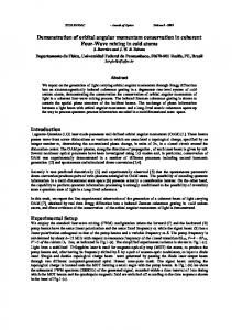
The special case α = 0, β = π/4, m0 = 1 of Eq. (18) is illustrated in Fig. 1 (see also Fig. 2 in Ref. [1]):
(13) (0,π/4)
2πV1,−1
(θ, p) 0.5
with the associated transition probability ˆ
(α, ˆ β) 2 |(χ(α,β) m0 ,m1 , χm0 ,m1 )| =
0.0 -0.5
(14)
1 ˆ ), cos2 β cos2 βˆ + sin2 β sin2 βˆ + sin 2β sin 2βˆ cos(α − α 2
ˆ for α which equals cos2 (β − β) ˆ = α. Eq. (14) is of interest in a discussion below (see Eq. (24)). According to Ch. IV of Ref. [1] the A-OAM Wigner function Vψ (θ, p) – here θ describes (by means of the pair (cos θ, sin θ)) the points on the (configuration) circle S1 of the classical phase space and p ∈ R the classical canonically conjugate OAM, ”V ” stands for “Vortex” – for a wave function ψ(ϕ) of Eq. (3) is given by Z π dϑ −ipϑ ∗ 1 e ψ (θ − ϑ/2) ψ(θ + ϑ/2). (15) Vψ (θ, p) = 2π −π 2π Taking for ψ(ϕ) the wave function (8) gives 2π Vm(α,β) (θ, p) 0 ,m1
1.0 0.5 0.0 −0.5 −1.0
−π
−π/2 θ
π
(17)
−π
(The remarkable significance of the sinc-function in the context of the A-OAM Wigner function is elaborately discussed in Ref. [1].) The third line in Eq. (16) represents the probability (α,β) (α,β) interference term in (χm0 ,m1 , χm0 ,m1 ) – see Eq. (9) – and describes, therefore, essential quantum mechanical properties of the state! Note that the interference term vanishes for p − (m0 + m1 )/2 = k, k ∈ {Z − {0}}. It vanishes, of course, too, if α or/and θ are such that cos[(m0 − m1 )θ − α] = 0. On the other hand, the last factor of the interference term is maximal (= 1) for p = (m0 + m1 )/2! The angles α and β may depend on other parameters, e.g., time t, space coordinates, external fields etc., and may, therefore, be manipulated from outside. Their values can be represented by points on the 2-dimensional surface of a “Bloch” sphere [12]. It is worthwhile to look at a few special examples: m1 = −m0 : (α,β)
2π Vm0 ,−m0 (θ, p) 2
(18) 2
= cos β sinc π(p − m0 ) + sin β sinc π(p + m0 )
+ sin 2β cos[2m0 θ − α] sinc π p.
p
m1 = 0 (ground state of H ∝ L2 ): (α,β)
2π Vm0 ,0 (θ, p)
(19) 2
where dϑ eixϑ .
0
−1
3
(α=0,β=π/4)
= cos2 β sinc π(p − m0 ) + sin β sinc π p
+ sin 2β cos[m0 θ − α] sinc π(p − m0 /2),
+ sin 2β cos[(m0 − m1 )θ − α] sinc π[p − (m0 + m1 )/2], sin πx 1 = πx 2π
−3
−2
2
(θ, p) = FIG. 1. A-OAM Wigner function 2π V1,−1 1 [sinc π(p − 1) + sinc π(p + 1)] + cos 2θ sinc πp of the qubit 2 √ (e+1 + e−1 )/ 2.
= cos2 β sinc π(p − m0 ) + sin2 β sinc π(p − m1 )
sinc πx =
π/2 π
(16)
Z
0
1
Here the interference term vanishes for p = m0 /2+k, k ∈ {Z − {0}}. (Recall that m0 6= 0 because m1 = 0.) The Wigner function (19) for the special values α = 0, β = π/3, m0 = 1 is shown in Fig. 2:
(0,π/3)
2πV1,0
(θ, p) 1.5 1.0 0.5
2.0 1.5 1.0 0.5 0.0 −0.5
−π
0.0
−π/2 θ
0 π/2 π
FIG. 2. 1 [sinc π(p 4
−3
−2
−1
0
2
(α=0,β=π/3)
√ 3 2
3
p
A-OAM Wigner function 2π V1,0
− 1) + 3 sinc πp] + √ qubit (e+1 + e0 )/ 2.
1
(θ, p) =
cos θ sinc π(p − 1/2) for the
The quantum mechanical marginal probability distri(α,β) butions |χm0 ,m1 (θ)|2 (angular distribution density) and 2 {cos β, sin2 β} (OAM distribution) of the state (8) can
3 be obtained, according to Ref. [1], from the A-OAM Wigner function (16) as follows: Z ∞ (θ, p) (20) dp Vm(α,β) 0 ,m1 −∞
1 = {1 + sin 2β cos[(m0 − m1 )θ − α]} 2π 1 = |χ(α,β) (θ)|2 2π m0 ,m1 – compare Eq. (9) –, where the relation Z ∞ dp sinc π(p + a) = 1, a ∈ R,
L2 (S1 × S1 , dϕ1 dϕ2 /(2π)2 ),
(21)
−∞
emn (ϕ) ˜ = em (ϕ1 ) en (ϕ2 ) = eimϕ1 +inϕ2 , m, n ∈ Z, (28) scalar product Z
−π
= cos β sinc π(p − m0 ) + sin β sinc π(p − m1 ), from which the quantum mechanical OAM probabilities cos2 β and sin2 β can be extracted immediately with the help of the orthonormality relations [1] Z ∞ dp sinc π(p − m) sinc π(p − n) = δmn . (23) −∞
ˆ (α, ˆ β) Vm0 ,m1 (θ, p)
(α,β)
π
(ψ2 , ψ1 ) =
2
2
(27)
with basis
has been used. Integration over θ gives Whittaker’s cardinal function [1] Z π (α,β) dθ Vm(α,β) (θ, p) = ωm (p) (22) 0 ,m1 0 ,m1 −π
Configuration space is now the torus S1 × S1 . A crucial tool for the derivation of the Wigner function (15) in Ref. [1] are the unitary representations of the Euclidean group E(2) of the plane [14]. In our case, ˜ p˜), we have to employ the direct product E(2) × P 4 (θ, E(2) and the associated unitary representations. The procedure for deriving the A-OAM Wigner function in question is then stricly analogue to that of Ch. II in Ref. [1] for the expression (15) and the result is as expected: We have the Hilbert space
d2 ϕ˜ ∗ ψ (ϕ)ψ ˜ 1 (ϕ), ˜ (2π)2 2
(29)
(ekm , eln ) = δkl δmn , and expansions X ψ(ϕ) ˜ = cmn emn (ϕ), ˜ cmn = (emn , ψ).
(30)
m,n∈Z
The functions (28) are eigenfunctions of the total OAM operator:
are A-OAM Wigner If Vm0 ,m1 (θ, p) and functions of the qubits (8) and (12), then the transition probability (14) is now given [1] by the integral Z ∞ Z π ˆ ˆ β) 2π dp dθVm(α,β) (θ, p)Vm(α, (θ, p) = (24) 0 ,m1 0 ,m1
Comparison of the basis (28) with Eqs. (6) and (7) suggests the following choice of correspondences:
1 ˆ ), cos β cos βˆ + sin2 β sin2 βˆ + sin 2β sin 2βˆ cos(α − α 2
em0 n0 ↔ |00i, em1 n1 ↔ |11i,
−∞
2
−π
2
where the relations (23), (21) and Z ∞ dp sinc2 π(p + a) = 1, a ∈ R,
(25)
−∞
have been used [13]. For the discussion of the tensor product of the Hilbert space L2 (S1 , dϕ/2π) from above – characterized by the Eqs. (1)–(3) – with itself we have to go slightly beyond the A-OAM framework discussed in Refs. [1, 2]: There we had a phase space P 2 (θ, p) = {(θ, p) ∈ S1 × R} with the circle S1 as configuration space and the real line R as cotangent space. Coordinates for the former are provided by the pair (cos θ, sin θ) and the angular momentum p ∈ R for the latter. By doubling the system we get the phase space ˜ p˜) ={(θ1 , θ2 ; p1 , p2 ) ∈ S1 × S1 × R × R)}, P (θ, θ˜ ≡ (θ1 , θ2 ), p˜ ≡ (p1 , p2 ). 4
(26)
L=
1 1 Lϕ + Lϕ2 , Lemn = (m + n)emn . i 1 i
(31)
(32)
em0 n1 ↔ |01i, em1 n0 ↔ |10i. Applying the same arguments of Ch. II in Ref. [1] – which lead to the Wigner function (15) – now to the ˜ p˜) and E(2) × E(2) we then get, on the products P 4 (θ, phase space P 4 for the wave function ψ of Eq. (30) the A-OAM Wigner function ˜ p˜) ≡ Vˆψ (θ, ˜ p˜)/(2π)2 = Vψ (θ, (33) Z π 2˜ d ϑ −i(p1 ϑ1 +p2 ϑ2 ) ∗ ˜ ˜ 1 ˜ e ψ (θ − ϑ/2) ψ(θ˜ + ϑ/2), (2π)2 −π (2π)2 which is the obvious generalization of the expression (15). We now want to determine the A-OAM Wigner functions for the general elements ψ2qb (ϕ) ˜ = c00 em0 n0 (ϕ) ˜ + c10 em1 n0 (ϕ) ˜ + c01 em0 n1 (ϕ) ˜ + c11 em1 n1 (ϕ), ˜ |c00 |2 + |c01 |2 + |c10 |2 + |c11 |2 = 1.
(34)
4 of the 4-dimensional tensor product space Q4m0 m1 ,n0 n1 of the space (10) with itself. The four complex coefficients cjk may be parametrized by real numbers as follows: c00 = b00 , c10 = eiα10 b10 , c01 = eiα01 b01 , c11 = eiα11 b11 , αjk ∈ [0, 2π), bjk ∈ R, b200 + b210 + b201 + b211 = 1. (35) Inserting the wave function (34) into the expression (33) yields the most general 2-qubit A-OAM Wigner function ˜ p˜) Vˆψ2qb (θ,
(36)
= b200 sinc π(p1 − m0 ) sinc π(p2 − n0 ) + b210 sinc π(p1 − m1 ) sinc π(p2 − n0 ) + b201 sinc π(p1 − m0 ) sinc π(p2 − n1 ) + b211 sinc π(p1 − m1 ) sinc π(p2 − n1 )
+ 2 b00 b10 cos[(m1 − m0 )θ1 + α10 ]
× sinc π[p1 − (m0 + m1 )/2] sinc π(p2 − n0 )
+ 2 b00 b01 cos[(n1 − n0 )θ2 + α01 ]
× sinc π(p1 − m0 ) sinc π[p2 − (n0 + n1 )/2]
+ 2 b00 b11 cos[(m1 − m0 )θ1 + (n1 − n0 )θ2 + α11 ]
× sinc π[p1 − (m0 + m1 )/2] sinc π[p2 − (n0 + n1 )/2]
+ 2 b01 b10 cos[(m1 − m0 )θ1 − (n1 − n0 )θ2 + α10 − α01 ]
× sinc π[p1 − (m0 + m1 )/2] sinc π[p2 − (n0 + n1 )/2]
+ 2 b01 b11 cos[(m1 − m0 )θ1 + α11 − α01 ]
× sinc π[p1 − (m0 + m1 )/2)] sinc π(p2 − n1 )
+ 2 b10 b11 cos[(n1 − n0 )θ2 + α11 − α10 ]
× sinc π(p1 − m1 ) sinc π[p2 − (n1 + n0 )/2].
(α11 ,β) ˜ V00,11 (θ, p˜) 1 {cos2 β sinc π(p1 − m0 ) sinc π(p2 − n0 ) = (2π)2
(38)
+ sin2 β sinc π(p1 − m1 ) sinc π(p2 − n1 )
+ sin 2β cos[(m1 − m0 )θ1 + (n1 − n0 )θ2 + α11 ]
× sinc π[p1 − (m0 + m1 )/2] sinc π[p2 − (n0 + n1 )/2]}.
It follows that the two basic entangled EPR/Bell states (α11 =0,β=±π/4) ˜ (6) have the Wigner functions V00.11 (θ, p˜) and (α10 −α01 =0,β=±π/4) ˜ the states (7) a corresponding V10,01 (θ, p˜). What is remarkable here is that the four entangled EPR/Bell states (6) and (7) do have irreducible A-OAM Wigner functions, i.e. they cannot be written as products of “lower” ones like in Eq. (37)! We see that this irreducibility of their Wigner functions is characteristic for EPR/Bell states! Considerable simplifications are obtained for the terms in expression (36) if m0 +m1 = 0, n0 +n1 = 0, m0 6= 0 6= n0 , and additionally n0 = m0 and αjk = 0 as well. This corresponds to a physical situation where a system with total angular momentum zero is decomposed or decays into two subsystems which move in opposite directions, one with angular momentum m0 and the other with m1 = −m0 . Example is a particle of spin zero which - in its rest frame - decays into 2 photons with opposite spins one. Examples with the simplifications mentioned: The A-OAM Wigner function for the basis vector em0 m0 (ϕ) ˜ is given by 1 [sinc π(p1 − m0 ) sinc π(p2 − m0 )]. (2π)2 (39) This follows from Eq. (36) with b00 = 1, b01 = b10 = b11 = 0. According to the correspondences (32) we get for the EPR/Bell states ˜ p˜) = Vm0 m0 (θ,
Here it is quite remarkable that in case of the four 2-dimensional specializations (b00 , b10 , b01 , b11 ) = (cos β, sin β, 0, 0), (cos β, 0, sin β, 0), (0, 0, cos β, sin β) or (0, cos β, 0, sin β) the Wigner function (36) factorizes into a qubit Wigner function (16) with θ = θ1 (or θ = θ2 ) and p = p1 (or p = p2 ) times Wigner functions Vn0 (θ, p) = sinc π(p − n0 )/(2π) etc. of the basis vectors en0 , en1 , em0 , or em1 [1]. We have, e.g., (α10 ,β) ˜ (θ, p˜) V00,10
(0, cos β, sin β, 0), where we get for the former
(37)
ψ00,11;± (ϕ) ˜ 1 = √ [em0 (ϕ1 )em0 (ϕ2 ) ± e−m0 (ϕ1 )e−m0 (ϕ2 )], 2 L ψ00,11;± (ϕ) ˜ = (2m0 ∓ 2m0 ) ψ00,11;± (ϕ), ˜
(40)
(41)
from Eq. (38) (with α11 = 0, β = ±π/4) the A-OAM 1 Wigner functions = {cos2 β sinc π(p1 − m0 ) + sin2 β sinc π(p1 − m1 ) (2π)2 ˜ p˜) Vˆ00,11;± (θ, (42) + sin 2β cos[(m1 − m0 )θ1 + α10 ] sinc π[p1 − (m0 + m1 )/2]} 1 ,β) = [sinc π(p1 − m0 ) sinc π(p2 − m0 )] × sinc π(p2 − n0 ) = Vm(α010 ,m1 (θ1 , p1 ) Vn0 (θ2 , p2 ). 2 1 + [sinc π(p1 + m0 ) sinc π(p2 + m0 )] 2 No such factorization occurs for the “entangled” cases ± cos[2m0 (θ1 + θ2 )] sinc πp1 sinc πp2 . – compare Eqs. (6) and (7) – (cos β, 0, 0, sin β) and
5 For the states ψ01,10;± (ϕ) ˜ (43) 1 = √ [em0 (ϕ1 )e−m0 (ϕ2 ) ± e−m0 (ϕ1 )em0 (ϕ2 )], 2 L ψ01,10;± (ϕ) ˜ = 0, (44) we get accordingly ˜ p˜) Vˆ01,10;± (θ, 1 = [sinc π(p1 − m0 ) sinc π(p2 + m0 )] 2 1 + [sinc π(p1 + m0 ) sinc π(p2 − m0 )] 2 ± cos[2m0 (θ1 − θ2 )] sinc πp1 sinc πp2 .
(45)
in the irreducibility of their A-OAM Wigner functions, which itself is related to the topology of the toroidal con˜ p˜). figuration subspace of the phase space P 4 (θ, Let us look at some details of the expression (45), with the minus sign in Eq. (43) and the related one in Eq. (45) as well: Integrating V01,10;− in Eq. (45) over p1 and p2 gives, with the help of relation (21): Z ∞ ˜ p˜) = dp1 dp2 V01,10;− (θ, (48) −∞
1 1 {1 − cos[2m0 (θ1 − θ2 )]} = {2 sin2 [m0 (θ1 − θ2 )]} 4π 2 4π 2 1 ˜ 2, = |ψ01,10;− (θ)| 4π 2
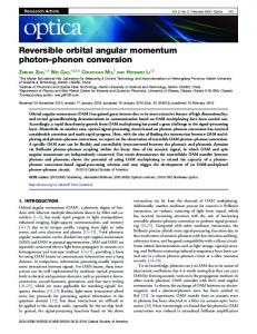
A special example of the function (45) with m0 = 1 at p2 = 1/2 is shown in Fig. 3.
(2π)2 V01,10;− (θ1 , θ2 , p1 , p2 = 1/2)
that is, the integral (48) gives the marginal angle probability density, as required by the general theory [1]. On the other hand, the angle integral Z π ˜ p˜) dθ1 dθ2 V01,10;− (θ, (49) −π
0.5
1 [sinc π(p1 − m0 ) sinc π(p2 + m0 )] 2 1 + [sinc π(p1 + m0 ) sinc π(p2 − m0 )] 2 = ω01,10;− (˜ p) =
0.0 -0.5
1.0 0.5 0.0 −0.5 −1.0
−π
−π/2 θ1 − θ2
0 π/2 π
−3
−2
−1
0
1
2
gives Whittaker’s cardinal function [1] for two variables p1 and p2 . Again, using the orthonormality relations (23), the marginal OAM probabilities
3
p1
|c01 |2 =
FIG. 3. Wigner function (2π)2 V01,10;− (θ1 , θ2 , p1 , p2 = 1/2) = 1 {− 13 sinc π(p1 −1)+sinc π(p1 +1)−2 cos[2(θ1 −θ2 )] sinc πp1 } π of the EPR/Bell state ψ01,10;− (ϕ) ˜ from Eq. (43).
Note again the θ-dependences in Eqs. (42) and (45): The Wigner functions of the entangled EPR/Bell states depend on both angles θ1 and θ2 , either only on the sum θ1 + θ2 or the difference θ1 − θ2 , respectively. Consider the curve C− ={θ− = θ1 − θ2 ∈ R; θ1 + θ2 = µ = const.,
(46)
4
p˜ = const.} ⊂ P (θ1 , θ2 , p1 , p2 ),
so that θ1 = (θ− + µ)/2, θ2 = (−θ− + µ)/2.
(47)
That means, if θ− increases then θ1 increases and θ2 decreases at the same rate, i.e. the curve (46) spirals around a torus. We see that non-classical properties of the EPR/Bell states (6) and (7) amazingly have their correspondence
1 1 , |c10 |2 = 2 2
(50)
can be extracted from ω01,10;− (˜ p). Special additional properties are: ˜ p1 , p2 ) = 0 for p1 , p2 ∈ {Z − {0}}, V01,10;− (θ,
(51)
and ˜ p1 , p2 = 0) Vˆ01,10;− (θ,
(52)
= − cos[2m0 (θ1 − θ2 )] sinc πp1 , with the corresponding relation for p1 = 0. This shows that the “classical” probabilities (50) as derived from Whittaker’s cardinal function (49) do not get any contributions from the phase space subsets p1 = 0 and p2 = 0 respectively, only the interference term does! A graphical illustration of the function (52) with m0 = 1 is given by Fig. 4. Furthermore, V01,10;− (θ1 , θ2 , p1 = 0, p2 = 0) = −
1 cos[2m0 (θ1 − θ2 )], 4π 2 (53)
6 [10] M. P. Van Exter, E. R. Eliel, and J. P. Woerdman, “Quantum entanglement of orbital angular momentum,” Ch. 16 of Ref. [7]. [11] M. Krenn, M. Malik, M. Erhard, and A. Zeilinger, “Orbital angular momentum of photons and the entanglement of Laguerre–Gaussian modes,” Phil. Trans. R. Soc. A 375, 20150442 (2017). [12] Page 15 of Ref. [3] and page 46 of Ref. [4]. [13] For Eq. (25) see the literature on the sinc function as quoted in Ref. [1]. [14] For details see the discussion in Ch. II of Ref. [1].
(2π)2 V01,10;− (θ1 , θ2 , p1 , p2 = 0) 0.5 0.0 -0.5
1.0 0.5 0.0 −0.5 −1.0
−π
−π/2 θ1 − θ2
0 π/2 π
−3
−2
−1
0
1
2
3
p1
FIG. 4. Wigner function (2π)2 V01,10;− (θ1 , θ2 , p1 , p2 = 0) = − cos[2(θ1 − θ2 )] sinc πp1 , according to Eq. (52) with m0 = 1, of the EPR/Bell state ψ01,10;− (ϕ) ˜ from Eq. (43).
showing explicitely that the Wigner function is negative on certain subsets of the phase space. I very much thank the DESY Theory Group for its sustained and very kind hospitality after my retirement from the Institute for Theoretical Physics of the RWTH Aachen. I am grateful to Hartmann R¨ omer for a stimulating discussion and to David Kastrup for providing the figures.
∗
[email protected] [1] H. A. Kastrup, “Wigner functions for the pair angle and orbital angular momentum,” Phys. Rev. A 94, 062113 (2016). [2] H. A. Kastrup, “Wigner functions for angle and orbital angular momentum: Operators and dynamics,” Phys. Rev. A 95, 052111 (2017). [3] M. A. Nielsen and I. L. Chuang, Quantum Computation and Quantum Information, 10th Anniversary Edition (Cambridge University Press, Cambridge, UK, 2010). [4] S. M. Barnett, Quantum Information, Oxford Master Series in Atomic, Optical and Laser Physics (Oxford University Press, Oxford, UK, 2009). [5] Ref. [3], Ch. 1 and Ref. [4], Ch. 2. [6] L. Allen, S. M. Barnett, and M. J. Padgett, eds., Optical Angular Momentum (Institute of Physics Publishing, Bristol and Philadelphia, 2003) a collection of reprints with introductory remarks for the different chapters. [7] D. L. Andrews and M. Babiker, eds., The Angular Momentum of Light (Cambridge University Press, Cambridge, UK, 2013) a collection of original review articles. [8] “Optical orbital angular momentum,” Phil. Trans. R. Soc. A 375, issue 2087 (2017), . Topical issue with introduction and 13 original articles, edited by S. M. Barnett, M. Babiker and M. J. Padgett. [9] S. M. Lloyd, M. Babiker, G. Thirunavukkarasu, and J. Yuan, “Electron vortices: Beams with orbital angular momentum,” Rev. Mod. Phys. 89, 035004 (2017).