Wilson Loop and Dimensional Reduction in Non-Commutative Gauge

Wilson Loop and Dimensional Reduction in

arXiv:hep-th/0104232v5 16 Aug 2001

Non-Commutative Gauge Theories

Sunggeun Lee1 and Sang-Jin Sin

2

Department of Physics, Hanyang University, Seoul, Korea

Abstract Using the AdS/CFT correspondence we study UV behavior of Wilson loops in various noncommutative gauge theories. We get an area law in most cases and try to identify its origin. In D3 case, we may identify the the origin as the D1 dominance over the D3: as we go to the boundary of the AdS space, the effect of the flux of the D3 charge is highly suppressed, while the flux due to the D1 charge is enhenced. So near the boundary the theory is more like a theory on D1 brane than that on D3 brane. This phenomena is closely related to the dimensional reduction due to the strong magnetic field in the charged particle in the magnetic field. The linear potential is not due to the confinement by IR effect but is the analogue of Coulomb’s potential in 1+1 dimension.

1 2

[email protected] [email protected]

1

1

Introduction

Recently, Maldacena[1] (See [2, 3] for a review) conjectured that string theory on AdS space-time is dual to SU(N) SYM, named AdS/CFT correspondence. If we turn on a NS B field on the N folding D-brane world volume, the low energy effective theory is equivalent to a noncommutative U(N) Super Yang-Mills(NCSYM) theory [4, 5, 6, 7, 8, 9, 10]. The corresponding dual gravity solution with nonvanishing B field was constructed in [11] as a bound state of branes. A Wilson loop can be calculated by the minimal area whose boundary is the given Wilson loop[12]. In non-vanishing B-field background, it is observed that the string tilts from its usual direction (orthogonal to the boundary of AdS) by certain angle so that the length of the string along the boundary is infinite[13]. Wilson loop that goes deep into the near horizon (IR) was found to give a Coulombic potential. In [14], it was observed that for a string moving with special velocity, the tilting angle is zero and the effect of the non-commutativity is merely renormalizing the Coulomb potential. So far, however, it is not clear why one should calculate the Wilson loop behavior at a fine tuned velocity. The unusual feature of the Wilson loops in the presence of the B field are associated with non-locality of the boundary gauge theory and the lack of the gauge invariance of the Wilson loop[15, 16, 17]. The super gravity solution is not asymptotically AdS5 space: the noncommutative directions shrink near the boundary. So there are some skepticism whether one can extract any physics out of the Wilson loop in non-commutative gauge theory. In recent paper of Dhar and Kitazawa [18], it is noticed that if we place the boundary at the finite position u = Λ, we can find a branch that gives the Coulomb potential and the situation looks as a small deformation of the commutative case. The price for having such branch is that the string configuration is not uniquely determined for a given length of Wilson line unless one put the probe brane at the non-commutative scale, u ∼ 1/a. If we put the probe brane at 1/a, we are cutting out

all the ”non-commutative region” (strong B-field region) in the bulk. Therefore it is not surprising that they get the Coulomb’s law for large Wilson line. Small Wilson line, whose Nambu-Goto string stays near the boundary, can ’feel’ the effect of the B field. In this case they find the area law. So they got the transition from Coulomb to area law as the size of the wilson line changes from large to small. Although interesting, the physics of the area law is not clear at all in this approach, especially because they cut out the all the strong B-field region. In this paper, we try to identify the mechanism of the area law. If the area law is a character of the the non-commutativity, we can expect that we should get it for any Wilson line which stay in the large B field region. So we do not put the boundary at the finite u. We put it at infinity as usual. As a consequence, the Coulomb branch, is not available to us. We will probe the non-commutative regime where the minimum point of the string, u0 , is larger than the non-commutatve scale, 1/a, so that entire Nambu-Goto string of the Wilson line is in the strong B-field region. We will find that the Wilson line follows universal area law. This is contrasted with the case of commutative case,

2

where temporal loop gives Coulomb’s law while spatial loop gives an area law [1, 3, 19, 20, 21]. In the presence B field case, we will show that we get area law for both case. In D3 case, we may identify the the origin as the D1 dominance [22, 23] over the D3: as we go to the boundary of the AdS space, the effect of the flux of the D3 charge is highly suppressed, while the flux due to the D1 charge is enhenced. So near the boundary, the theory is more like a theory on D1 brane than that on D3 brane. This phenomena is closely related to the dimensional reduction due to the strong magnetic field in the charged particle in the magnetic field. Then, the linear potential is not due to the confinement by IR effect but is the ’analogue’ of Coulomb’s potential in 1+1 dimension. This paper is organized as follows. In section 2, we review the gravity dual of non-commutative gauge theory and its scaling symmetries. In section 3, we calculate the Wilson loop in UV regime for various cases including finite temperatures, spatial as well as temporal loops, D-instanton background and other Dp brane cases. We get an area law almost universally if time is not non-commutative. In section 4, we give a physical interpretation for the area law of 3+1 dimensional non-commutative gauge theories as D1 dominance and dimensional reduction due to the magnetic field. We summarize and conclude in section 5.

2

Gravity dual of the non-commutative gauge theory and its scaling symmetry

Let us first consider the zero temperature case of D3 brane with constant B field parallel to the brane. Its low energy effective world-volume theory is described by noncommutative Yang-Mills theory. The gravity dual solution in string frame is given in [11, 13, 24]. Its solution is bound state solution of D3 and D1 branes and is given by 1

1

ds2s = f − 2 [−dx20 + dx21 + h(dx22 + dx33 )] + f 2 (dr 2 + r 2 dΩ25 ), α′ 2 R4 , h−1 = sin2 θf −1 + cos2 θ, r4 sin θ −1 B23 = f h, cos θ e2φ = g2 h, 1 1 F01r = sin θ∂r f −1 , F0123r = cos θh∂r f −1 . g g

f =1+

(2.1)

The above solution is asymptotically flat for r → ∞ and they have a horizon at r = 0. In region near

r = 0 the solution has a form AdS5 × S 5 . In order to obtain non-commutative field theory we should

take the B field to infinity. In the decoupling limit α′ → 0 with finite fixed variables u=

r α′ R2

˜b ˜b , ˜b = α′ tan θ, x ˜2,3 = ′ x2,3 , gˆ = ′ g, α α

3

(2.2)

and the metric becomes ds

2

′

= αR

2

"

2

u

n

−dx20

+

dx21

#

o du2 2 ˆ x2 + d˜ + h(d˜ x ) + 2 + dΩ25 , 2 3 u

1 , a2 = ˜bR2 , a + a4 u4 2 α′ a4 u4 ′R = α , B = , B∞ ∞ ˜b 1 + a4 u4 a2 ˆ gˆ2 h, ˜b α′ u4 R4 , gˆ ˆ 2h α′ ∂u (u4 R4 ), gˆ

ˆ = h ˜23 = B e2φ = A01 = F˜0123u =

(2.3)

where gˆ is the value of the string coupling in the IR and R4 = 4πˆ g N . This is the gravity dual solution to NCSYM. For small u which corresponds to IR regime of gauge theory the metric reduces to ordinary AdS5 × S 5 . This is consistent with the expectation that the noncommutative Yang-Mills reduces to

ordinary Yang-Mills theory at long distances(IR). The solution starts deviating from the AdS space p at u ∼ a1 , i.e. at a distance scale ∼ R ˜b. For large R4 where supergravity limit is valid, this is greater p than the naively expected distance scale of L ∼ ˜b. So the effects of non-commutativity is visible at longer distances than naively expected. The metric has a boundary at u = ∞. As we approach to the

boundary, the physical scale of the 2,3 direction shrinks. In this region it seems that only D1 brane is

relevent. The non-commutative nature arise from the fact that the position of D1 in D3 is not fixed but widely fluctuating. We now discuss the symmetry property of the metric. In the absence of B field, the metric is that of the well known AdS5 × S 5 . 2

′

ds = α R

2

"

u

2

(−dx20

+

dx21

+

dx22

+

dx23

+

dx23 )

du2 + 2 + dΩ25 u

#

(2.4)

This metric has a rescaling symmetry at the boundary xµ → λxµ , (µ = 0, 1, 2, 3) and u →

u λ

(2.5)

This symmetry is associated with the U V /IR: large in x corresponds to the small in u. In the presence of B field, however, the metric near the boundary has the form ds2 = α′ R2

"

#

du2 1 u2 (−dx20 + dx21 ) + 2 (dx22 + dx23 ) + 2 + dΩ25 . u u

(2.6)

At the boundary the noncommutative directions shrink and the metric effectively becomes that of AdS3 . This has the scaling symmetry at the boundary x0,1 →

1 0,1 x , x2,3 → λx2,3 , and u → λu, λ 4

(2.7)

which is slightly different from that of the zero B field case. Therefore the co-ordinate distance L along the non-commutative direction near the boundary u = U corresponds to the physical length x2,3 /aU [18].

3

Wilson loops in various cases

In this section we consider temporal Wilson loop at finite temperature in non-commutative gauge theory. The gravity dual is a non-extremal blackhole background with B dependence [13]. The metric is given by 

ds2 = α′ R2 u2

(

)



u4 du2 2 2 ˆ −(1 − h4 )dx20 + dx21 + h(dx + dΩ25  . 2 + dx3 ) + u4h u 2 u (1 − u4 )

(3.1)

Here tildes are omitted for convenience. String theory on this background should provide a dual description of non-commutative Yang Mill theory at finite temperature. For small u, the metric is reduced to that of the AdS-Schwarzschild black hole. Let u0 be the smallest possible value of u on the Wilson loop in the bulk. This gravity dual solution can be trusted when the following conditions are satisfied. • small string coupling:

gˆ eφ = q ≪ 1, 1 + a4 u40

• small curvature :

gˆY2 M N = gˆN ≫ 1.

(3.2)

(3.3)

We know from the above gravity solution, that au0 ∼ 1 is a transition region from AdS5 blackhole

region to dimensionally reduced AdS3 region. Let u0 be the minimal value available to the string configuration. The noncommutative effect is relevant to au0 ≫ 1(UV) region. Since it is expected

to get Coulomb’s law for au0 ≪ 1(IR) where the noncommutaive effect is invisible, it is expected

to get something else for the quark-antiquark potential, like an area law. We will show indeed this is so by calculating the Wilson loops in various cases and also we will find necessary condition for this to happen. There is agreements that IR behaviour is Coulombic [13, 14, 18], while there are different opinions for the UV behavior. Therefore our interest will be for au0 ≫ 1(UV) where the noncommutative effect is manifest in the metric behavior (a ∼ ˜b).

3.1 3.1.1

Wilson loops in non-commuative gauge theory at finite temperature Temporal loop

Now consider classical string world-sheet action, Nambu-Goto action, which is given by S=

1 2πα′

Z

dσdτ 5

q

det(hαβ ),

(3.4)

where hαβ = GM N ∂α X M ∂β X N . We choose static gauge as τ = x0 , σ = x2 , u = u(σ). Then on the background of (3.1), we have hτ τ = α′ R2 u2 (1 −

u4h ), u4

hτ σ = hστ = 0, ˆ + α′ u−2 (1 − hσσ = α′ R2 u2 h

u4h −1 ) (∂σ u)2 . u4

(3.5)

So the Nambu-Goto action can be written as R2 S= T 2π

Z

q

ˆ 4 − u4 ) + (∂x u)2 . dx2 h(u 2 h

(3.6)

The action does not explicitly depend on x2 so it gives

q

ˆ 4 − u4 ) h(u h

ˆ 4 − u4 ) + (∂x u)2 h(u 2 h

= c.

(3.7)

ˆ 0 . Then we can determine At u = u0 , where it is the closest point to the horizon, ∂x2 u = 0 and ˆh → h

c

ˆ 0 (u4 − u4 ). c2 = h 0 h

(3.8)

This allows us to write x2 as a function of u x2 =

s

u40 − u4h 1 + a4 u4h

Z

4

s

For large u, x2 ∼ a

du q

1 + a4 u4 (u4 − u40 )(u4 − u4h )

.

u40 − u4h u = ku, 1 + a4 u4h

(3.9)

(3.10)

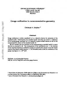
where k can be interpreted as a slope for large u. This implies that we cannot fix the position of the string at infinity since x2 grows linearly with u. See figure 1. This dependence of u is associated to

L

u=infinity

u=u_0 u=0 u=u_h

¯ separation L grows indefinitely since x3 = ku as we approaches to the boundary. Figure 1: QQ

6

non-locality[25] of noncommutative theory. In the IR region we get the Coulombic potential by similar calculation of [14]. However, we will soon see that in the UV region (au0 ≫ 1) we get different one. L and u0 is related by

v u u u 1− L = x2 (u → ∞) = t

2

where y =

u u0 .

u4h u40 a4 u4h

1+

1 u0

Z

1

∞

1 + a4 u40 y 4 dy r (y 4 − 1)(y 4 −

u4h ) u40

,

(3.11)

The energy of this configuration is given by

E=

R2 π

s

v

4 u Z ∞ u y 4 − uh4 t 1 + a4 u40 u0 dy u0 y4 − 1 1 + a4 u4h 1

.

(3.12)

For uh a ≤ u0 a ≪ 1, it is known that we get the screened Coulomb potential [19, 12].

We are currently interested in the UV regime (au0 ≫ 1) where the noncommutative effect is crucial. When we consider au0 ≫ 1 case (equivalently uh /u0 → 0), L and E are respectively given by "

L 1 ∼ a4 u40 2 u0

Z

1

∞

#

R2 2 2 y2 , and E ∼ a u0 · u0 dy p 4 π y −1

Then the relation between E and L can be read.

E=

Z

∞

1

y2 . dy p 4 y −1

R2 L πa2

(3.13)

(3.14)

Both separation length and energy are infinite and there is no canonical way to renormalize the separation length. If all what we want is the E − L relation, the only reasonable way to regularize

both quantity is to put a cutoff in u. The question is whether we can give a physical interpretation to this. We will try this at section 4. For a moment, we just calculate the the Wilson loops for various other situations.

3.2

Spatial loop

Spatial Wilson loops in high temperature are interesting since they can be considered as ordinary Wilson loops of Euclidean field theory in one less dimension. 3.2.1

In three dimension

Let us start with the Euclidean non-extremal D3-brane metric with B23 fields. The metric has the form as before 

(

ds2 = α′ R2 u2 (1 −

u4h 2 )dt u4 E

)

2 2 ˆ + dx21 + h(dx 2 + dx3 ) +

du2 u2 (1 −

u4h u4 )



+ dΩ25  .

(3.15)

Compactify this four dimensional theory on S1 of tE by periodically identify its period with the inverse Hawking temperature proportional to uh and take high temperature limit so that the radius 7

becomes zero. The resulting effective theory is then interpreted as Euclideanized three dimensional noncommutative field theory. The circle compactification breaks both supersymmetry and conformal symmetry. After compactifying tE , the resulting three dimensional theory is described by coordinates x1 , x2 , and x3 . Among them, for instance, x1 can be considered as a Euclideanized time and x2 , x3 as spatial coordinates. For the spatial loop, the string configuration we use is τ = x1 ,σ = x2 and u = u(σ). Then the Nambu-Goto action become T R2 S= 2π ˆ= where h

1 1+a4 u4 .

Z

s

ˆ + (1 − dx2 u4 h

u4h −1 ) (∂x2 u)2 , u4

(3.16)

Then it is easy to show that the separation length 2 L= u0

∞

Z

1

1 + a4 u40 y 4 dy r (y 4 − 1)(y 4 −

u4h ) u40

.

(3.17)

and energy E=

q

R2 u0 1 + a4 u40 Z 2π

∞

1

y4 dy r (y 4 − 1)(y 4 −

u4h ) u40

.

(3.18)

¿From these, the relation between E and L when the noncommutative parameter au0 is E∼

R2 L. 2πa2

(3.19)

In case of B = 0, the spatial loop is gives an area law, while the temporal loops are not. Here (B 6= 0),

both give the area law when the noncommutative parameter is large. 3.2.2

Four dimensional case

Here we start with non-extremal D4-brane. The metric with B fields[13] is given by 1

1

ds2 = f − 2 [dx20 + dx21 + h(dx22 + dx23 ) + dx24 ] + f 2 (dr 2 + r 2 dΩ24 ),

(3.20)

where 3

α′ 2 R3 f =1+ , h−1 = f −1 sin2 θ + cos2 θ, r3 B23 = f −1 h tan θ, e2φ = g2 f

−1 2

h.

(3.21)

The decoupling limit exists and is given by r = α′ R2 u, α′ → 0, ˜b −1 α′ ˜i , a3 = ˜b2 α′ 2 R3 , tan θ = ′ , xi = x ˜b α ′ 3 3 ˜23 = α a u . B ˜b 1 + a3 u3 8

(3.22)

For non-extremal case the metric is simply written as ds2 =

"

1 ′4

1 2

α′ R2 (α R u )−1 u2 1 ′4

1 1+a3 u3

(

u3 2 2 2 ˆ (1 − h3 )dt2 + dx21 + h(dx 2 + dx3 ) + dx4 u 

du2

1 2

1 2

+(α R u )( ˆ= where h

1 2

u2 (1

−

+ dΩ24 ) ,

u3h u3 )

)

(3.23)

and tildes are ommited for convenience. For static string configuration τ = x1 , σ =

x2 , u = u(σ), the Nambu-Goto action can be written as T R2 S= 2π

Z

s

dx2 α′

−1 2

ˆ + (1 − R−1 u3 h

u3h −1 ) (∂x2 u)2 . u3

(3.24)

The first integral is 1

ˆ α′ 2 R−1 u3 h q

α′

−1 2

ˆ+ R−1 u3 h

(1 −

= c,

u3h −1 2 u3 ) (∂x2 u)

(3.25)

ˆ 0 . After some calculation, the separation length where c2 = α′ −1/2 R−1 u30 h −1

2u02

L= q −1 α′ 2 R−1

Z

∞

1

1 + a3 u30 y 3 dy r (y 3 − 1)(y 3 −

u3h ) u30

,

(3.26)

and the energy E=

q

R2 u0 1 + a3 u30 Z π

∞

1

For UV-regime au0 ≫ 1, we again get an area law. E=

y3 dy r (y 3 − 1)(y 3 −

R3 1

α′ 2 π 2 a3

3.3

!1

u3h ) u30

.

(3.27)

2

L.

(3.28)

Wilson loop in D-instanton background

In this section we consider one more example: quark-antiquark potential in D-instanton background with constant B field. The gravity dual solution for B = 0 was considered in [26]. It is easy to turn on B field for this background. First rotate the D-instanton background and then T -dualize it. Then the resulting metric[27] is given by 1

h

ds2 = H 2 f where

−1 2

n

o

1

i

dt2 + dx21 + h(dx22 + dx23 ) + f 2 (dr 2 + r 2 dΩ25 ) ,

α′ 2 qα′ 4 R4 , H = 1 + , r4 r4 e2φ = g2 hH, B23 = f −1 hH tan θ, 1 h= . 2 −1 Hf sin θ + cos3 θ

(3.29)

f =1+

9

(3.30)

This D-instanton is smeared over D3 brane worldvolume. This solution is T -dual to D4+D0 or D5+D1(with B field) brane configuration. In the decoupling limit r = α′ R2 u, α′ → 0, ˜b q 2 tan θ = ′ , f → (α′ R4 u4 )−1 , H → 1 + 4 4 , a2 = ˜bR2 , α R u ˜b2 a4 u4 h → ′2 , , B23 → H (1 + Ha4 u4 ) α (1 + Ha4 u4 ) α′ ˜ . x0,1 = x ˜0,1 , x2,3 = x ˜b 2,3

(3.31)

So the metric becomes #

"

o n 1 q du2 2 ˆ x2 + d˜ ds = α R (1 + 4 4 ) 2 u2 d˜ + dΩ25 ) , x20 + d˜ x21 + h(d˜ x ) + ( 2 3 R u u2 2

ˆ= where h

1 1+Ha4 u4

′

2

and H = 1 +

q R4 u4 .

(3.32)

The metric becomes flat R10 as u → 0 while it deviates from

flat as u become large. When B field is zero, this metric solution describes wormhole solution which connects flat space(R10 ) in u → 0 with AdS 5 × S5 in u → ∞.

For the static string configuration, τ = x0 , σ = x2 , and u = u(σ), the Nambu-Goto action can be

written as

R2 T 2π which gives the following first integral. S=

Z

q

ˆ + (∂x u)2 }, dx2 H{u4 h 2 √

ˆ Hu4 h

q

ˆ + (∂x u)2 u4 h 2

(3.33)

= c,

(3.34)

ˆ 0 . L and E are given by where c2 = H0 u40 h L 2

q

(1 +

=

q ) R4 u40

Z

∞

dy

(1 + a4 y 4 u40 +

qa4 R4 )

p , y2 y4 − 1 s Z ∞ (y 2 + 4 q2 4 ) qa4 R2 R y u0 4 4 dy p 1 + a u0 + 4 u0 . 4 π R y −1 1

E =

u0

1

(3.35)

Here our interest lies in the region where au0 ≫ 1 and u0 ≫ uh , L∼

a4 u30

Z

1

∞

a2 R2 u30 y2 , and E ∼ dy p π y4 − 1

which after elimination of u0 gives

Z

1

∞

y2 dy p , y4 − 1

(3.36)

R2 L. (3.37) πa2 One should notice that in UV region, u > u0 > 1/a, the D-instanton effect is negligible and the E=

non-commutativity effect is dominant. The fact that the D-instanton charge is proportional to α′4 is crucial to neglect the D-instanton effect in the UV region. 10

For B = 0, it is known [26] that the large L correspond to (u0 → 0) and it leads to an area law.

To compare this and above case let’s look at some details. In this case L and E is given by √ 3s s Z 1 L q 1 ∞ q 1 2 2π 2 dy 2 p 4 = 1+ 1+ 4 4 , = 1 4 2 2 Ru0 u0 1 R u0 u0 Γ( 4 ) y y −1 R2 π

"Z

!

#

y2 R2 1 E = dy p 4 −1 −1 + π u30 y −1 1 √ √ √ 2R2 π 2R2 u0 π + . = − Γ( 4q )2 u30 Γ( 41 )2 ∞

As u0 → 0, L → ∞, we have E=

Z

∞

1

dy

y2

1 y4 − 1

p

R4 √ L. 2π q

(3.38)

(3.39)

Although 3.37 and 3.39 gives similar results the details are very different. B = 0 case is the IR result (u0 ≪ 1) and is a consequence of dynamics, while B 6= 0 case is the UV result and kinematical.

3.4

General Dp brane cases

In order to study more general case, we look at the Wilson loop in higher dimensional non-commutative Yang-Mill theories. The dual gravity metric is given by [13] ds2 = Hp−1/2 [h0 (−dx20 + dx21 ) + h1 (dx22 + dx23 ) + · · ·] + Hp1/2 [du2 + u2 dΩ25 ]

(3.40)

with Hp ∼ 1/u7−p and hi = 1/(ai u)4 . We again, do not need to consider the black holes since we are

interested in large au0 ≫ 1 case. The general string action is S∼T

Z

q

dx h0 (H −1 h + (∂x u)2 ).

(3.41)

Here we assumed that the string is along x direction which is one of the non-commutative planes. We immediately see that as u → ∞, H −1 h → constant, resulting in the linear potential if and only if

h0 = constant, namely of no B01 field is applied. This can be easily verified if we observe that when h0 is constant the action (3.41) leads to the first integral (∂x u)2 + f (1 − f /f0 ) = 0

(3.42)

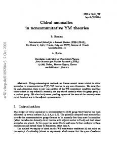
where f (u) = H −1 (u)h(u) and f0 is the value of f at u = u0 . The qualitative behavior of the solution can be read off from the particle moving with zero energy under the potential f (1 − f /f0 ). See figure

2. The effect of D3 brane charge (F5 flux H(u)) is to pull out the particle to the boundary of AdS, while that of NS-NS charge (B23 field h(u)) is to pull in the particle into the horizon. In terms of boundary variable, the former expands the xµ along the brane directions, while the latter shrink the x2 , x3 plane. The essence of the phenomena is the exact cancellation of two effect in the asymptotic region. Since both H and h are based on the harmonic power u−(7−p) of the transverse dimensions, this is unavoidable in the region where those terms are dominant. The net effect is such that the particle has a constant speed, or the Wilson loop has a constant slope. 11

0.25 0.2 0.15 0.1 0.05 4

2

6

8

10

Figure 2: The minimal surface problem is reduced to the motion of a classical particle moving with 0 total energy in a potential V = f (1 − f /f0 ). The potential peak is near the 1/a. In the plot, we set a = 1, u0 = 3.

4

D1 dominance and Dimensional reduction

Now we want to figure out the origin of the linear behavior of the potential in more physical terms for the interested D3 case. Consider the metric for following class: 2

′

ds = α R

2

"

2

u

h0 (−dx20

+

dx21 ) +

u

2

h1 (dx22

+

dx23

+

dx23 )

du2 + 2 + dΩ25 u

#

(4.1)

where hi = 1/(1 + (ai u)4 ). For large au0 ≫ 1 and u0 ≫ uh , we do not need to care about the black

hole effect. The non-commutativity effect (B field effect) is dominant. The string action is S∼T

Z

q

dx2 h0 (u4 h1 + (∂x u)2 ).

(4.2)

For the case we considered, h0 = 1 and h1 ∼ 1/u4 , so that the action becomes S ∼ T /a

Z

s

1+(

du 2 ) , dx

(4.3)

after the scaling u → u/a and x → ax. Therefore the energy is proportional to the line element of

flat space. The shortest length is for the straight line. Therefore since the line is not orthogonal to the boundary, the energy has to be proportional to the linear length in the x-direction. What happen if we turn on B01 also? In this case non-trivial h0 arise [13]. The metric for large u region is that of AdS5 × S 5 [13]; 2

′

ds = α R

2

"

−dx20 + dx21 + dx22 + dx23 + du2 + dΩ25 u2

#

(4.4)

which is the metric of AdS5 × S 5 ( but in Poincare co-ordinate). So it is similar to the near horizon

geometry of distributed D-instanton over the D3 [13, 26, 28]. The boundary u = ∞ is now at the

AdS-horizon. In fact one can show that the critical path with the given boundary condition does not exist. From the calculational point of view, what is crucial for the area law is the absence of h factor 12

in the gtt . However this means that g11 is also free of the h factor. Therefore we have to have one spatial direction along which B field is not applied to get the area law. According to the super gravity solution (2.1), there is a D1 branes along x1 direction. Furthermore, near the boundary, the existence of D3 brane is suppressed by h ∼ 1/u4 factor relative to the D1 branes. F01r =

1 sin θ∂r f −1 , g

F0123r =

1 cos θh∂r f −1 . g

(4.5)

In near horizon limit, ˜b F01u = α′ ∂u (u4 R4 ), gˆ ′2 ˆ · α ∂u (u4 R4 ) F˜0123u = h gˆ

(4.6)

Another manifestation of the D1 dominance[22, 23] near the boundary is the metric itself. The near horizon limit of the metric shows that g22 , g33 is suppressed by the same factor h ∼ 1/u4 compared

to the g11 . In fact this suppression of the non-commutative direction is the motivation to begin this

work. The non-commutativity in x2 , x3 can be interpreted as the fluctuation of the the location of the D1 brane along those directions. In fact this is origin of the fluctuation of the end point of the Wilson line noted in [13]. One may further understand the behaviour of Wilson loop by considering the open string as dipole [29, 30] and taking the analogy to the charged particle in magnetic field. In case of charged particle, when F23 is applied, the particle stay in the lowest Landau level and only transverse x1 direction is available for the free motion. This is so called ’dimensional reduction’ due to the magnetic field. The particle moves in the effective 1+1 dimension whose kinematic effect gives Coulomb’s law of linear potential. This is closely parallel to the fact in metric: g22 and g22 is highly suppressed relative to gtt and g11 .

5

Summary and Discussion

In this paper, we study the UV behaviour of the Wilson loop in the non-commutative gauge theory. The Wilson loop calculation in AdS/CFT is reduced to the particle dynamics in a potential defined by the D3 brane charge and NS-NS B field. In spite of the the lack of the gauge invariance of the Wilson loops in non-commutative gauge theory, a physically meaningful aspect of Wilson loop comes out. After calculating various cases, we observed that the area law in the UV region is universal if no B01 is applied and it is consequence of balance of two competing tendency: the effect of F5 flux (H(u)) is to pull out the particle to the boundary of AdS, while that of B23 (h(u)) is to pull in the particle into the horizon. In case of D3 brane, the effect has striking similarity with so called dimensional reduction and ’Magnetic Catalysis’, where strong magnetic field project the electron states to its lowest Landau 13

level so that the charged particle has reduced degrees of freedom: it is effectively 1+1 dimensional system[31, 32]. If the magnetic field F23 is turned on, the x2 , x3 plane is effectively confining the electron motion and the system undergoes dimensional reduction, which in turn causes chiral symmetry breaking of a massless fermion system. Apparently, the similarity between the charged particle and open string in strong magnetic field is not complete, since the string is dipole rather than a charge. If the string aligned along the x1 direction transverse to the non-commutative plane, it does not see the dimensional reduction at all. However, the Wilson line we discussed is with zero velocity and the particle with zero velocity does not feel any magnetic field nor the dimensional reduction, either. So, the parallelism is stronger than expected. So, it would be interesting to study whether magnetic catalysis phenomena exist in the 3+1 dimensional non-commutative field theory.

Acknowledgements This work was supported by Korea Research Foundation Grant (KRF-2000-015-DP0081) and by Brain Korea 21 Project in 2001.

References [1] J.M.Maldacena, The Large N Limit of Superconformal Field Theories and Supergravity , Adv.Theor.Math.Phys.2(1998)231, hep-th/9711200; N.Itzhaki, J.M.Maldacena, J.Sonnenschein and S.Yankielowicz,Supergravity and The Large N Limit of Theories with Sixteen Supercharges, Phys.Rev.D58(1998)046004, hep-th/9802042. [2] O.Aharony, S.S.Gubser, J.M.Maldacena, H.Ooguri and Y.Oz, Large N Field Theories, String Theory and Gravity, Phys.Rept.323(2000)183, hep-th/9905111. [3] P.Di Vecchia,Large N gauge theories and AdS/CFT correspondence, hep-th/9908148 [4] M.R.Douglas and C.Hull,D-branes and the Noncommutative Torus, JHEP9802(1998)008, hepth/9711165 [5] A.Connes, M.Douglas and A.Schwarz,Noncommutative Geometry and Matrix Theory: Compactification on Tori, JHEP 9802(1998)003, hep-th/9711162 [6] F.Ardalan, H.Arfaei, and M.M. Sheikh-Jabbari,Noncommutative Geometry From Strings and Branes, JHEP 9902(1999)016, hep-th/9810072 [7] M.M.Sheikh-Jabbari,Super Yang-Mills Theory on Noncommutative Torus from Open Strings Interactions, Phys.Lett.B450(1999)119,hep-th/9810179 [8] V.Schomerous, D-branes and Deformation Quantization, JHEP 9906(1999)030, hep-th/9903205 14

[9] C.Chu and P.Ho, Constrained Quantization of Open String in Background B Field and Noncommutative D-brane, Nucl.Phys.B568(2000)447, hep-th/9906192 [10] N.Seiberg and E.Witten, String Theory and Noncommutative Geometry, JHEP 9909(1999)032, hep-th/9908142 [11] R.C.Myers,More D-brane bound states, Phys.Rev.D55(1997)6438, hep-th/9611174; M.S. Costa, and G. Papadopoulos, Superstring dualities and p-brane bound states. Nucl.Phys. B510 (1998) 217-231, hep-th/9612204; J.P.Gauntlett, D.A.Kastor and J.Trachen,Overlapping Branes in MTheory, Nucl.Phys.B478(1996)544, hep-th/9604179; A.A.Tseytlin, Harmonic superpositions of M-branes, Nucl.Phys.B475(1996)149, hep-th/9604035. [12] J.Maldacena, Wilson loops in large N field theories, Phys.Rev.Lett.80(1998)4859, hep-th/9803002; S.-J.Rey and J.Yee,Macroscopic Strings as Heavy Quarks of Large N Gauge Theory and Anti-de Sitter Supergarvity, hep-th/9803001 [13] J.Maldacena and R.Russo,Large N Limit of Non-Commutative gauge Theories,JHEP 9909(1999) 025, hep-th/9908134 [14] M.Alishahiha, Y.Oz and M.M.sheikh-Jabbari, Supergravity and Large N Noncommutative Field Theories, JHEP 9911(1999)007, hep-th/9909215 [15] Sumit R. Das, Soo-Jong Rey, Open wilson lines in noncommutative gauge theory and tomography of holographic dual supergravity, Nucl.Phys.B590: 453-470, 2000, hep-th/0008042 [16] Sumit R. Das, Sandip P. Trivedi, Supergravity couplings to noncommutative branes, open wilson lines and generalized star products, JHEP 0102:046,2001, hep-th/0011131 [17] D.Gross, A.Hashimoto and N.Itzhaki, Observables of Non-Commutative gauge Theories, hepth/0008075 [18] A.Dhar and Y.Kitazawa,Wilson loops in strongly coupled noncommutative gauge theories, to appear in Phys.Rev.D, hep-th/0010256 [19] S.-J.Rey, S.Theisen and J.Yee, Wilson-Polyakov Loop at Finite Temperature in Large N Gauge Theory and Anti-de Sitter Supergravity, Nucl.Phys.B527(1998)171, hep-th/9803135; A.Brandhuber, N.Itzhaki,J.Sonnenschein and S.Yankielowicz, Wilson Loops in the Large N Limit at Finite Temperature, Phys.Lett.B434(1998)36, hep-th/9803137;ibid, Wilson Loops, Confinement, and Phase Transitions in Large N Gauge Theories from Supergravity, JHEP9806(1998)001, hep-th/9803263 [20] J.Sonnenschein, What does the string/gauge correspondence teach us about Wilson loops?, hepth/0003032 15

[21] E.Witten, Anti-de Sitter Space, Thermal Phase Transition, And Confinement In Gauge Theories,Adv.Theor.Math.Phys.2(1998)505, hep-th/9803131 [22] J.X. Lu and S. Roy, (p + 1)-Dimensional Noncommutative Yang-Mills and D(p − 2) Branes, Nucl.Phys. B579 (2000) 229-249, hep-th/9912165

[23] Rong-Gen Cai and Nobuyoshi Ohta, Noncommutative and Ordinary Super Yang-Mills on (D(p − 2), Dp) Bound States, JHEP 0003 (2000) 009, hep-th/0001213 .

[24] A.Hashimoto and N.Itzhaki, Non-Commutative Yang-Mills and the AdS/CFT Correspondence , Phys.Lett.B465(1999)142 ,hep-th/9907166 [25] D.Biggati

and L.Susskind,

Magnetic fields,

branes and noncommutative geometry,

Phys.Rev.D62(2000)066004, hep-th/9908056 [26] H.Liu and A.A.Tseytlin, D3-brane-D-instanton configuration and N=4 YM theory in constant self-dual background, Nucl.Phys.B553(1999)231, hep-th/9903091 [27] J.G.Russo and M.M.Sheikh-Jabbari, Strong Coupling Effects in non-commutative spaces fron OM theory and supergarvity, hep-th/0009141 [28] C. Park and S.-J.Sin ,Notes on D-instanton correction to AdS5 × S 5 geometry, Phys. Lett. B444 (1998)156-162, hep-th/9807156

[29] Sheikh-Jabbari, Open Strings in a B-field Background as Electric Dipoles, Phys. Lett. B 455 (1999) 129-134 [30] John McGreevy, Leonard Susskind and Nicolaos Toumbas, Invasion of the Giant Graviton from Anti-de Sitter Space, JHEP 0006 (2000) 008, hep-th/0003075. [31] V.P. Gusynin, V.A. Miransky and I.A. Shovkovy Phys. Rev. Lett.73(1994)3499-3502,Catalysis of Dynamical Flavor Symmetry Breaking by a Magnetic Field in 2 + 1 Dimensions, hep-ph/9405262 [32] Deog Ki Hong, Youngman Kim, Sang-Jin Sin, RG analysis of magnetic catalysis in Dynamical symmetry breaking, Phys.Rev.D54(1996) 7879-7883, hep-th/9603157

16