2016 7th International Renewable Energy Congress (IREC)
Modeling and Control of PV/Wind Microgrid Ashraf Khalil*, Khalid Ateea Alfaitori, and Ali Asheibi Electrical and Electronics Engineering Department Faculty of Engineering, University of Benghazi Benghazi, Libya
[email protected] magnetic synchronous generator (PMSG). Many machines can be connected to the wind turbine. For large wind farms the induction generator is the most widely used. For isolated systems such as the Microgrid the PMSG is used because there is no need to excitation current from the grid. Additionally PM machines are more efficient and have higher energy yield. Both the PV array and wind energy system is connected to a 3 phase voltage source inverter. These inverters are connected in parallel and the control strategy has to stabilize the system and achieve good power sharing. Additionally the voltage, the phase and the frequency must be kept within predetermined ranges.
Abstract—Microgrids are becoming the de facto for future power system. This paper presents the modeling and control of PV/Wind Microgrid. Renewable energy sources such as PV, wind and fuel cells are usually connected through voltage-source inverters. In order to share the same loads these inverters are connected in parallel to form a Microgrid. The system considered in the paper consists of two parallel inverters fed with PV array and wind turbine. The PV array and the wind turbine are variable nonlinear DC sources and hence the control system should achieve good power sharing even with this imperfections. The controller is designed in the dq reference frame where the Space Vector Pulse Width Modulation is used. The first inverter contains outer voltage control loop and inner current control loop while the second inverter contains only power control loop. The controller is tested through simulation where the PV array and the wind system produce different DC levels. The simulation results show that the power sharing is achieved. Keywords— parallel inverter; stability; microgrid; SVPWM; photovoltaic; wind
I.
PV Array
Load
INTRODUCTION
Power system is evolving in the form of Microgrid. The ever growing increased energy demands and the energyrelated environmental problems of fossil fuel made the renewable energy resources one of the most viable alternatives for the large centralized fossil-fueled power plants. Recently distributed energy sources, such as fuel cells, wind turbines and photovoltaic cells are integrated to form a Microgrid [1]. Microgrid is a system of parallel inverters that can be connected to the grid. Distributed power sources in MG must operate in parallel in order to share the loads. Among renewable energy sources in MG, wind and photovoltaic (PV) systems are smaller and more scalable which made them suitable to be integrated generators into MG. PV system is one of the exciting new technologies to convert sunlight directly into electricity. According to the learning curve the cost reduction of PV system will continue in the future [2]. PV/Wind MG is proven to be one of the forms of future evolution of the grid. A PV/Wind Microgrid is shown in Figure. 1. The PV source is a series and parallel connections of PV modules. PV modules can be connected to the grid in different configurations such as the central, string and multistring. Due to its low cost and its simplicity the centralized configuration is used for large installations where the PV array is connected to a central inverter. The wind turbine is connected to the rectifier through a permanent
3 Phase VSI
LC filter
3 Phase VSI
LC filter
PMSG Wind Turbine
Rectifier
Fig. 1.
A system of two parallel inverters
There are many reviews on the control strategies in Inverterbased MGs (see [3], [4], [5] and the references therein). The control strategies can be classified into centralized, distributed, master-slave and decentralized control strategies [3]. In the centralized control strategy, all the information is sent to a central controller and then the commands are sent back to the system. However the current sharing is achieved at all times, the system is vulnerable to the single point of failure [3]. Additionally the system needs high bandwidth communication link, and is sensitive to nonlinear loads [3]. In order to solve the problems associated with the controller's interactions, decentralized control was introduced. In decentralized control only local information are used in the decentralized controller. One of the widely used decentralized control methods is the Droop control [4]. The main idea is to
978-1-4673-9768-1/16/$31.00 ©2016 IEEE
1
2016 7th International Renewable Energy Congress (IREC)
regulate the voltage and the frequency by regulating the reactive and the active power respectively that can be sensed locally. The Droop control method has many desirable features such as expandability, modularity, redundancy, and flexibility. There are as well some drawbacks such as, slow transient response and possibility of circulating currents. As the interconnections are neglected the overall system stability cannot be guaranteed.
similar to the normal diode. When sunlight with energy greater than the semiconductor energy gap hits the cell electrons becomes free and a considerable current flows in the external circuit. As PV cells are fragile and have low voltage they grouped into modules and encapsulated from front and supported by metallic panel for protection. The modules are then connected in series and parallel to form an array as shown in Figure 2. There are many methods in the literature for modeling PV modules [9, 10 and 11]. The model used in this paper is based on the single-diode model and extracting some of the parameters from the manufacturer data sheet. The electrical circuit model is shown in Figure 3.
In the master-slave control strategy, one of the converters is known to be the master while the others are the slaves, the master controller contains the voltage controller while the slaves contain current controllers and have to track the master’s reference current [5]. Master/Slave control strategy gives a good load sharing and synchronization. The distributed control is adopted in this paper. In the distributed control strategy the rotational reference frame (dq0) is used instead of the stationary reference frame (abc). The voltage controller controls the output voltage by setting the average current demands [3]. In current/power sharing control method the average unit current can be determined by measuring the total load current and divide this current by the number of units in the system. The load sharing is forced during transient and the circulating currents are reduced. Additionally lower-bandwidth communication link is needed. The distributed control strategy is adopted in this paper. Many researchers reported master-slave and distributed control strategies that rely on shared-network for control signals exchange [6, 7 and 8].
Fig. 2.
The paper starts from the description of the PV/Wind MG. Then the mathematical model of the parallel inverters, the PV array and wind energy system are presented. The PV array is a series and parallel connection of PV modules. The model of the PV module is the single diode five parameters model. The PV module model is implemented in Matlab/Simulink. The wind turbine is connected to a PMSG. The PMSG is then connected to the 3 phase VSI through uncontrolled rectifier. The distributed control strategy is briefly explained where the space vector pulse width modulation (SVPWM) is used. One of the main issues in inverter based MG is the stability of the system. The controller parameters are selected to stabilize the parallel inverters and achieve good performance. A simulation using Matlab/SimPowerSystems toolbox is carried out to test the effectiveness of the control strategy where each inverter is connected with different renewable source. II.
A pn-junction silicon solar cell
Fig. 3.
Circuit model of a solar cell
The model is with middle complexity where the temperature dependence of I0, Iph, and Voc are included. Also the parasitic resistances Rs and Rsh and their temperature dependence are taken into account. The ideality factor is used as a variable to match the simulated data with the manufacturing data. The mathematical model of a solar cell based on the single diode model is given as: I (T , G ,V ) = I ph - I 0 (e (V + IR ) / nV - 1) - (V + I × Rs ) / Rsh s
th
= I ph - I D - I sh
where the variables in (1) are given by [10]; I ph = I ph0 × G / Gnom
MATHEMATICAL MODEL OF PV/WIND MICROGRID
The typical circuit of two parallel three-phase voltage source inverters fed through 10 kWp PV array and 20 kW wind turbine is shown in Figure. 1. The controller has to stabilize the system and to have a good power sharing even when the sources have different DC values. This is the situation when the inverters are connected with different renewable sources.
(2)
I ph (T ) = I ph + K0 (T - Tmeas )
(3)
K0 = ( I ph (T2 ) - I ph (T1 )) /(T2 - T1 )
(4)
I 0 = I SC (T ) × (T / T1 )
(5)
3/ n
1
× exp( - E g / Vs (1 / T - 1 / T1 ))
I 0 (T1 ) = I SC (T ) /(exp( qVOC (T ) / nkT1 ) - 1) 1
OC
qVOC ( T1 ) / nkT1
1
)
(7)
Rsh = VOC /( I ph - I 0 [exp(qVOC / nkTmeas - 1])
(8)
Rsh (T ) = Rsh × (T / Tmeas )
(9)
a
2
(6)
1
Rs (T ) = -dV / dIV - 1/( I 0 (T ) × q / nkT1 × e
A. The Mathematical Model of The PV Array PV solar cells rely on the photoelectric effect to generate electricity. The basic PV cell is the p-n junction shown in Figure 2. In the dark the characteristics of the PV cell is
(1)
2016 7th International Renewable Energy Congress (IREC)
The parameters in the model are explained briefly. Iph is the photo generated current in Amperes. Iph0 is the photo generated current at the nominal radiation. I0 is the diode dark saturation current. ID is the diode dark current. Ish is the shunt current. Rs is the series resistance. Rsh is the shunt resistance. G is the solar radiation in W/m2. The Gnom is the radiation the PV module is calibrated at. n is the ideality factor. e is the electron charge. k is Boltzmann's constant. Vg is the semiconductor energy gap. K0 is the short-circuit current temperature coefficient. Vth is the thermal voltage. The manufacturer provides the following: Ns: the number of cells in series, Np: the number of cells in parallel, Isc: the shortcircuit current, Voc: the open-circuit voltage. The Solarex MSX60 60W module is used in the simulation [12]. The equations from (1) to (9) are implemented in Matlab/Simulink.
electromagnetic torque. The specification of the PMSG are as follows: Ld = Lq = 0.95 mH, the stator resistance Rs=0.085 Ω, the inertia 0.08 Kg.m2, the viscous damping 0.001147 N. m. s, number of poles 4. The output electrical AC power of the PMSG is converted into DC power through the diode rectifier as shown in Figure. 5. Turbine output power (pu of nominal mechanical power)
Turbine Power Characteristics (Pitch angle beta = 0 deg)
The PV modules are connected in series and parallel to produce the required voltage and power. As our energy source is nonlinear the goal of the controller is to generate AC power with given voltage shape parameters and to achieve power sharing between the different inverters in the MG. The PV array used in the simulation has 10 branches with 22 modules in each branch and the total number of modules is 220.
1
Max. power at base wind speed (12 m/s) and beta = 0 deg 12 m/s
0.8 10.8 m/s 0.6 9.6 m/s 0.4
8.4 m/s 7.2 m/s 6 m/s
0.2
1 pu
0 -0.2 -0.4 0
Fig. 4.
0.2
0.4 0.6 0.8 1 1.2 Turbine speed (pu of nominal generator speed)
1.4
The mechanical power versus the turbine speed
B. The Mathematical Model of the Wind Turbine The mechanical power of the wind turbine is given by [13]: Pm = 0.5 rAC p v w3
(10) PMSG
where P m the mechanical power in watts, ρ is the air density (Kg/m3), A is the swept area (m2) and Cp is the power coefficient of the turbine, vw is the wind speed (m/s). The power coefficient represents the conversion efficiency of the turbine. If the pitch angle β=0, Cp is function of the tip speed, λ, of the turbine and is given by [13]: C p (l ) = c1 (
c2 - c 4 ) e - c5 / l + c 6 l l
Wind Turbine
Fig. 5.
~ ~ ~ ~ d é id 1 ù 1 éd d1 ù 1 évd ù é 0 - w ù é id 1 ù ê ~ ú = ê ~ úVdc1 - ê ~ ú - ê ú × ê~ ú L1 ëvq û ëw 0 û êë iq1 úû dt êë iq1 úû L1 êë d q1 úû ~ ~ ~ ~ d é id 2 ù 1 éd d 2 ù 1 évd ù é 0 - w ù é id 2 ù = × V ê ~ ú dc 2 ê~ ú ê ú ê ú ê~ ú dt ëê iq 2 ûú L2 ëê d q 2 ûú L2 ëv~q û ëw 0 û ëê iq 2 ûú é 1 ù ~ ~ ~ ~ d évd ù 1 æç é id 1 ù é id 2 ù ö÷ ê RC - w ú évd ù × ê~ ú + ê ~ ú - ê ê ú= 1 ú êëv~q úû dt ëv~q û 2C çè ëê iq1 ûú ëê iq 2 ûú ÷ø ê w ú RC û ë
C. The Permanent Magnetic Synchronous Generator The mathematical model of the PMSG is given by [14]: di q / dt = vq / Lqs - ( rs / Lqs )iq + ( Lds / Lqs )w e id - (y f w e / Lqs ) Te = 1 .5 p ( Lds - Lqs )id iq + iqy
The wind turbine connected to a rectifier through PMSG
D. The Mathematical Model of the Parallel Inverters The average model of the phase leg is derived based on the switching averaging. After transformation of the variables in the stationary coordinates Xabc into the rotating coordinates Xdqz, the average model can be simplified [15, 16 and 17] based on iz= iz1 = -iz2 ≈ 0:
(11)
where λ=ωR/vw, ω is the rotational speed (rad/s), R is the radius of the blades. The maximum power can be extracted from the turbine can be achieved when cp=0.48 and λ=8.1. The coefficients c1 to c6 are: c1 = 0.5176, c2 = 116, c3 = 0.4, c4 = 5, c5 = 21 and c6 = 0.0068 [13]. The wind turbine used in the simulation has the following specification: power rating, 20 kW, the rated wind speed 12 m/s, cut-in and cut-out speeds 5 and 25 m/s respectively, blade diameter 10 m. The mechanical power of the wind turbine versus the generator speed for different wind speeds is shown in Figure 4.
di d / dt = v d / Lds - ( r s / Lds )i d + ( Lqs / Lds )w e i q
Rectifier
(12) (13)
Writing (15), (16) and (17) in general matrix form: ~ ~ x& = A~ x + Bu ~ ~ y = Cx
(14) where, Ld, Lq are d and q axis inductances, R is stator winding resistance, id, iq are d and q axis currents, vq, vd are d and q axis voltage, ω r is angular velocity of rotor, λm is amplitude of rotor induced flux, p is pole pair number, and Te is f
The state vector and the control vector are given as: ~ ~ ~ ~ ~ x = [v~d v~q id 1 iq1 id 2 iq 2 ]T
3
(15) (16)
(17)
(18) (19)
2016 7th International Renewable Energy Congress (IREC)
~ = [d~ u d1
~ ~ ~ d q1 d d 2 d q 2 ]T C = I, the matrices A, B can be obtained as: é- 1 / RC ê -w ê ê - 1 / L1 A=ê ê 0 ê - 1 / L2 ê êë 0
é0 ê 0 B=ê ê0 ê ë0
1 /( 2C ) 0 1 /( 2C ) 0 ù w 0 1 /( 2C ) 0 1 /( 2C )úú - 1 / RC 0 0 0 0 ú w ú 0 0 0 ú - 1 / L1 -w 0 0 0 0 w ú ú 0 0 0 úû - 1 / L2 -w
0 Vdc1 / L1 0 0
0 0
0
0 III.
0
0
ù ú 0 ú 0 ú ú Vdc1 / L1 û 0
Vdc1 / L1 0 Vdc1 / L1 0 0 0
(20)
T
(21)
THE DISTRIBUTED CONTROL
In the distributed control strategy the first and the second inverter have two control loops as shown in Figure. 6. The inner control loops independently regulate the inverter output current in the rotating reference frame, id and iq. The outer loop works in the voltage control mode to produce the d-q axis current references for the inner loop by regulating the voltage at given reference value. In power control mode, the outer loop is used to regulate the active and the reactive power at given operating points and provide the current references, id-ref and iq-ref, in the rotating reference frame for the inner loop ([16],[17]). The SVPWM is used to derive the six pulses where a PI controller scheme is used. The duty cycles signals are given as: ~ ~ ~ ~ (22) d d 1 × Vdc1 = K idp1 + K idi 1 / s id 1-ref - id 1 - wL1 iq1 + v~d ~ ~ ~ ~ (23) - i + wL i + v~ d ×V = K + K / s i q1
dc 1
( (
iqp 1
)( )(
iqi 1
q 1- ref
q1
) )
1 d1
Fig. 6.
The outputs of these outer controllers are the inputs of the inner control loops. A proportional controller is used, then we have: ~ id 2 - ref = K Pp 2 (Pref - P2 ) (30) ~ iq 2 - ref = KQp 2 (Qref - Q2 ) (31) In order to write the closed loop equation in matrix form, new control variables are introduced into (22)-(27). Then the new duty cycle signals can be expressed as: ~ ~ ~ d d 1 = (1 / Vdc1 )[(1 - Kidp1 Kvdp )~ vd - Kidp1 id 1 - wL1 iq1 (32) ~ + K K F + K g~ + K K v~ ] idp 1
q2
dc 2
iqp 2
iqi 2
q 2 - ref
q2
) )
2 d2
q
d1
idi 1
d1
idp 1
(
q2
dc 2
vdp
d - ref
)
(
iqp 2
Qp 2 d 2
)
q
iqp 2
Qp 2 q 2
d
~ ~ + (1.5 Kiqp 2 KQp 2 v~d - Kiqp 2 ) iq 2 - (1.5 Kiqp 2 KQp 2 v~q - wL2 )id 2 (35) ~ + K g~ + K K F ] iqi 2
q2
iqp 2
Qp 2
ref
The control output can be expressed as: ~~ ~ = H × ~z + J (v~ ~ u d vq P Q ) ref ~~~ ~ ~ ~ where; ~ z = [v~d v~q id 1 iq1 id 2 iq 2 F d 1F q1g~d 1g~q1g~d 2g~q 2 ]T
(36)
Substituting the control laws in the state equation and writing the equations in s-domain: -1 z( s) / R ( s) = (sI - A 1 - B 1 H ) × B 2 (37) ~~ where: R ( s ) = [(v~d v~q P Qref )]( s ) , A1 and B1 are the state and the input matrices of the closed loop system.
q
In the power control mode the active and the reactive power are controlled at given set points by the outer loops to produce the d-q axis current references for the inner loops ([16] and [17]). The active and the reactive power are given as: P = (3 / 2) Vd id 2 + Vd iq 2 (28) Q = (3 / 2) Vq id 2 - Vd iq 2 (29)
( (
vdi
~ ~ ~ d q1 = (1 / Vdc1 )[(1 - Kiqp1 Kvqp )v~q - Kiqp1 iq1 + wL1 id 1 ~ (33) + Kiqp1 Kvqi F q1 + Kiqi1g~q1 + Kiqp1 Kvqp v~q - ref ] ~ ~ ~ d d 2 = (1 / Vdc1 )[ 1 - 1.5 Kidp 2 K pp 2 id 2 ~ vd - 1.5 Kidp 2 K pp 2 iq 2 v~q ~ ~ - (1.5 Kidp 2 K pp 2 v~d + Kidp 2 ) id 2 - (1.5 Kidp 2 K pp 2 v~q + wL2 )iq 2 (34) ~ + Kidi 2g~d 2 + Kidp 2 K pp 2 Pref ] ~ ~ ~ d = (1 / V )[ 1 - 1.5 K K i v~ + 1.5K K i v~
The voltage control loop regulates the voltage and generates the d-q axis current references for the current loop. Therefore the output of the outer voltage controller is the input of the inner control loop, a proportional-integral (PI) controller is also used in the current control loop. Then: ~ id 1- ref = (K vdp + Kvdi / s )(v~d - ref - v~d ) (24) ~ (25) iq1- ref = (Kvqp + Kvqi / s )(v~q - ref - v~q ) The second inverter operates in the power control mode, where the instantaneous values of the inverter output current components id-ref and iq-ref are used to control the output active and the reactive power respectively as shown in Figure 6. The duty-cycle signals for the second inverter are given as: ~ ~ ~ ~ d d 2 × Vdc 2 = (Kidp 2 + Kidi 2 / s ) id 2 - ref - id 2 - wL2 iq 2 + v~d (26) ~ ~ ~ ~ ~ d × V = (K + K / s ) i - i + wL i + v (27)
( (
Closed-loop control of two Parallel Inverters
) )
4
2016 7th International Renewable Energy Congress (IREC)
IV. SIMULATION RESULTS
16000
The PV/Wind MG in Figure. 1 is implemented with Matlab/Simulink. The parallel inverters parameters are as follows: C=22 μF , L=4 mH and R = 4.25 ohm. In previous work the control parameters that achieve the optimum performance are determined [18, 19]. The controllers' parameters are: Kvdp=Kvqp=5, Kvdi=Kvqi=400, Kidp1=1, Kidi1=100, Kiqp1=0.4 and Kiqi1=60, Kpp2=5, Kqp2=5, Kidp2=1, Kidi2=100, Kiqp2=0.4 and Kiqi2=60. In the control strategy the second inverter is forced to generate 10 kW real power and 2 kVar reactive power. Figure 7 shows that the output three phase voltages of the parallel inverters maintained at 170 V peak value. In the simulation, the radiation on the PV array is fixed at 1000 W/m2 while the temperature is fixed at 25 C then the radiation is reduced at 0.15 s to 800 W/m2. The wind speed is fixed at 12 m /s while the pitch angle is zero. The operating point of the PV array is shown in Figure 8. The DC input voltages of the first and the second inverter are shown in Figure. 9. Reducing the radiation from 1000 W/m2 to 800 W/m2 forces the PV array to operate in new operating point. At 0.15 s when the radiation decreased to 800 W/m2 the voltage is 427.7 V. If the operating point stays at this point then the supplied power will be less than 10 kW. Hence the operating point changes to 394 V in order to generate 10 kW. The DC input currents of the inverters are shown in Figure. 10. The small oscillation in the DC bus is because of the switching characteristics of the inverters.
14000
First Operating Point of Array A and B
The Power, W
12000
X: 427.9 Y: 1.001e+04
10000
X: 394.9 Y : 1.041e+04
8000
Second Operating Point of A rray A
1000 W/m2
6000
800 W/m2
4000 2000 0
0
50
100
Fig. 8.
150
200
250 300 350 The Voltage, V
400
450
500
550
The PV curve of the two arrays
600
The PV array voltage The wind turbine voltage
500
The voltage, V
400
300
200
100
0
0
0.05
Fig. 9.
0.1
0.15 Time, (Seconds)
0.2
0.25
0.3
The DC input voltage of the inverters
140
200
120
150
100
The current, A
100
The Voltage, V
50
The PV array current The wind turbine current
80
60
40
0 20
-50
0
-100
-20
0
0.05
0.1
0.15 Time, (Seconds)
0.2
0.25
0.3
-150
-200
Fig. 10. 0
0.01
0.02
0.03
0.04 0.05 0.06 Time, (Seconds)
0.07
0.08
0.09
The DC input currents of the inverters
0.1
60
Fig. 7.
The three-phase output voltages 40
The first inverter current, the second inverter and the load current are shown in Figures. 11-13. We notice that there is no change in the currents at 0.15 and this is because at 800 W/m2 the array is still capable of supplying the required power. The output power of the first inverter and the second inverter are shown in Figure 14. The sharing between the inverters is good even during the transient but the first inverter supplies most of the current. In the simulation the nonlinear model of the inverters is implemented. The research in this paper is to be extended to deal with different renewable sources such fuel cells and batteries [19].
The Current, A
20
0
-20
-40
-60
0
0.01
Fig. 11.
5
0.02
0.03
0.04 0.05 0.06 Time, (Seconds)
0.07
0.08
0.09
The output currents of the first inverter
0.1
2016 7th International Renewable Energy Congress (IREC)
The current research is to test the controller strategy with different renewable sources such as fuel cells and batteries.
60
40
REFERENCES The Current, A
20
[1] 0
[2]
-20
-40
-60
0
0.01
Fig. 12.
0.02
0.03
0.04 0.05 0.06 Time, (Seconds)
0.07
0.08
0.09
[3]
0.1
The output currents of the second inverter
[4]
100 80
[5]
60
The Current, A
40 20
[6]
0 -20 -40 -60
[7]
-80 -100
0
0.01
0.02
Fig. 13.
0.03
0.04 0.05 0.06 Time, (Seconds)
0.07
0.08
0.09
0.1
[8]
The output currents of the load
[9]
20000 The The The The
The power, W
15000
active power of the first inverter reactive power of the first inverter active power of the second inverter reactive power of the second inverter
[10]
10000
[11] [12]
5000
[13] 0
[14] 0
Fig. 14.
0.05
0.1
0.15 0.2 Time, (Seconds)
0.25
0.3
[15] [16]
The active and the reactive power of first inverter
V. CONCLUSION
[17]
The paper deals with modeling and control of PV/Wind Microgrid. The model of the PV array and wind energy system are implemented in Simulink. A distributed control strategy is used to stabilize the system while achieve load sharing. The controller is tested and the power sharing is achieved even when the PV array and the wind energy system produce different DC levels. With this distributed control strategy the first inverter supplies most of the current during the transient.
[18]
[19]
6
B. Lasseter. "Microgrids [distributed power generation]", In Proceedings of 2001 Winter Meeting of the IEEE Power Engineering Society, 28 Jan.-1 Feb, Piscataway, NJ, USA: IEEE, pp. 146-149,2001. Friederike Kersten, Roland Doll, Andreas Kux, Dominik M.Huljic, Marzella A.Gorig, Christian Breyer, Jorg W.Müller, and Peter Wawer, "PV Learning Curves: Past and Future Drivers Of Cost Reduction," In the 26th European Photovoltaic Solar Energy Conference and Exhibition, At Hamburg, Germany, 2011. M. Prodanovic.,T. C. Green & H. Mansir.. "Survey of control methods for three-phase inverters in parallel connection". IEE Conference Publication (475), pp. 472-477, 2000. K. De Brabandere, B. Bolsens, J. Van den Keybus, A. Woyte, J. Driesen, and R. Belmans,"A voltage and frequency droop control method for parallel inverters", IEEE Transactions on Power Electronics, vol. 22, no. 4, pp. 1107-1115, 2007. S. K. Mazumder., M. Tahir, & K. Acharya. "Master-slave currentsharing control of a parallel dc-dc converter system over an RF communication interface". IEEE Transactions on Industrial Electronics, 55, (1) pp. 59-66, 2008. S. K. Mazumder, M. Tahir., & K. Acharya. "An Integrated Modeling Framework for Exploring Network Reconfiguration of Distributed Controlled Homogenous Power Inverter Network using Composite Lyapunov Function Based Reachability Bound". Simulation, 86, (2), pp. 75-92, 2010. Y. Wei, X. Zhang,,M. Qiao, & J. Kang, "Control of parallel inverters based on CAN bus in large-capacity motor drives", In 2008 Third IEEE International Conference on Electric Unity Deregulation, Piscataway, NJ, USA: IEEE, pp. 1375-1379, 2008. Yai Zhang, Hao Ma and Fei Xu, "Study on Networked Control for Power Electronic Systems", In the Proceedings of the Power Electronics Specialists Conference, Orlando, FL, USA, pp. 833-838, 2007. J. A. Gow, C. D. Manning, "Development of a photovoltaic array model for use in power-electronics simulation studies", lEE ProceedingsElectric Power Applications, Vol 146, No. 2, pp. 193-200, 1999. G. Walker, “Evaluating MPPT Converter Topologies Using a Matlab PV Model”, Journal of Electrical and Electronics Engineering, Australia, Vol. 21, No. 1, pp. 49-56, 2001. Hansen A. D., Sorensen P., Hansen L. H., Binder H., "Model for standalone PV system", Roskilde: Rio National Laboratory, 2000. Solarex MSX60 datasheet. Available online at: http://www.californiasolarcenter.org/newssh/pdfs/Solarex-MSX64.pdf Siegfried Heier, "Grid Integration of Wind Energy Conversion Systems," John Wiley & Sons Ltd, 1998, ISBN 0-471-97143-X Krause, P.C., O. Wasynczuk, and S.D. Sudhoff. Analysis of Electric Machinery and Drive Systems. IEEE Press, 2002. Zhihong Ye, "Modeling and Control of Parallel Three-Phase PWM Converters", PhD thesis, Virginia State University, September 15, 2000. Yu Zhang, "Small-Signal Modeling and Analysis of Parallel- Connected Power Converter Systems for Distributed Energy Resources" PhD thesis, University of Miami, 2011. Yu Zhang, Zhenhua Jiang, and Xunwei Yu, "Small-Signal Modeling and Analysis of Parallel-Connected Voltage Source Inverters" In the proceedings of the IEEE 6th confenerence on Power Electronic and Motion Control, pp. 377-383, May 17-20, 2009. Ashraf Khalil, Khalid Ateea and Ahmed El-Barsha, "Stability Analysis of Parallel Inverters Microgrid", The 20th International Conference on Automation and Computing (IEEE), UK, pp. 110-115, 2014. Ashraf Khalil and Khalid Ateea, "Modeling and Control of PhotovoltaicBased Microgrid", International Journal of Renewable Energy (IJRER), Vol. 3, No. 5, pp. 826- 835, 2015.