(top), the standard MCP method (middle) and the neural network based MCP (bot- tom). .... Tieleman, T.: Gnumpy: an easy way to use gpu boards in python.
Wind Power Resource Estimation with Deep Neural Networks Frank Sehnke1 , Achim Strunk2 , Martin Felder1 , Joris Brombach2 , Anton Kaifel1 , and Jon Meis2 1
Zentrum f¨ ur Sonnenenergie- und Wassersto↵-Forschung, Industriestr. 6, 70565 Stuttgart, Germany 2
EWC Weather Consult GmbH, Sch¨ onfeldstrae 8, 76131 Karlsruhe, Germany
Abstract. The measure-correlate-predict technique is state-of-the-art for assessing the quality of a wind power resource based on long term numerical weather prediction systems. On-site wind speed measurements are correlated to meteorological reanalysis data, which represent the best historical estimate available for the atmospheric state. The di↵erent variants of MCP more or less correct the statistical main attributes by making the meteorological reanalyses bias and scaling free using the on-site measurements. However, by neglecting the higher order correlations none of the variants utilize the full potential of the measurements. We show that deep neural networks make use of these higher order correlations. Our implementation is tailored to the requirements of MCP in the context of wind resource assessment. We show the application of this method to a set of di↵erent locations and compare the results to a simple linear fit to the wind speed frequency distribution as well as to a standard linear regression MCP, that represents the state-of-the-art in industrial aerodynamics. The neural network based MCP outperforms both other methods with respect to correlation, root-mean-square error and the distance in the wind speed frequency distribution. Site assessment can be considered one of the most important steps developing a wind energy project. To this end, the approach described can be regarded as a novel, high-quality tool for reducing uncertainties in the long-term reference problem of on-site measurements.
1
Introduction
Due to the strong inter-annual variability of wind velocities in most regions that are interesting for wind power generation, reliable wind resource assessments require long-term time series for every specific location. Many approaches use data from meteorological reanalyses which represent the best historical estimate for the atmospheric state on regular grids. Moreover, these data sets allow for incorporating a sufficient length of the time series giving robust estimates in a climate context. Virtual time series at site level are produced by downscaling techniques, either using regional to local numerical model simulations including
2
Frank Sehnke et. al.
Computational Fluid Dynamics (CFD), or statistical or parametric methods, or combinations thereof. Finally these long-term time series are combined with local observations or measurements from representative locations nearby using a technique called Measure-Correlate-Predict (MCP). MCP is described by [1] as: “MCP methods model the relationship between wind data (speed and direction) measured at the target site, usually over a period of up to a year, and concurrent data at a nearby reference site. The model is then used with long-term data from the reference site to predict the long-term wind speed and direction distributions at the target site.” In recent years, however, meteorological reanalyses from Numerical Weather Prediction (NWP) systems became increasingly available. The correlation between reanalysis data for the site and the measurements at the site are much higher and so MCP is now used with NWP reanalyses but with the same techniques described in [1]. These techniques range from standard deviation correction (to remove the overall scaling error) over wind speed ratio corrections (to remove the overall bias) to vector regression and linear regression – the latter being the standard and therefore heavily employed in industrial aerodynamics. High quality MCPs enable reconstruction of the long-term historical wind resource using a limited number of observations while, at the same time, achieving reduced uncertainties. Due to the cost of gathering observations at site level and the need to have early, reliable estimates of future economic return, a stateof-the-art MCP and high-end long-term time series are key aspects during the initial phase of wind energy projects. The standard MCP variants fail, however, to utilize high order correlations of the long-term historical wind resource data with the limited number of observations. We show that Deep Neural Networks (DNN) [2] apparently make use of these higher order correlations. The implementation is fully tailored to the requirements of MCP in the context of wind resource assessment. We show the application of our method to a set of di↵erent locations and compare the results to a simple linear fit to the wind speed frequency distribution as well as to a standard linear regression MCP. The neural network based MCP outperforms both other methods with respect to correlation, root-mean-square error and the distance in the wind speed frequency distribution. Site assessment can be considered one of the most important steps developing a wind energy project. To this end, the approach described can be regarded as a novel, high-quality tool for reducing uncertainties in the long-term reference problem of on-site measurements. In the following sections we will introduce the long-term data under consideration as well as the observations used for this study. After a description of the DNN setup, di↵erent MCP variants will be introduced and the results will be compared to the method under consideration.
Wind Power Resource Estimation with Deep Neural Networks
2
3
Method
2.1
Long-term Data
EWC’s Wind Potential Analysis employs the reanalysis product from the MERRA project [3], which covers the time range from 1979 to the present. A parametric downscaling approach, which bases on [4], is applied to the hourly vertical wind profiles at a specific site. This approach takes into account, besides others, local orography inferred from high resolution digital elevation models. Using similarity theory, atmospheric stability and local vegetative roughness, individual hourly vertical wind profiles are calculated. The resulting wind velocities and directions then serve as artificial wind time series at (wind turbine) hub height. In this study the additional data sets of orography and land cover have a global resolution of roughly 1⇥1 km2 . The parametric downscaling approach within EWC’s Wind Potential Analysis is constantly being evaluated by numerous observational time series (e.g., [5]). In addition to resource assessment, this approach is also successfully applied for wind power forecast services [6]. 2.2
Observational Data
In the current study we present the application of the novel MCP to a number of di↵erent locations. The hourly wind speed observations are either based on nacelle anemometers at hub height or have been gathered on net masts. The time periods of available measurement data are given in Table 1. The locations have been chosen – due to their moderate skill in the initial long-term time series, and – aiming at representing di↵erent terrain characteristics ranging from o↵-shore over near-shore flat to on-shore, complex and a↵ected by forests. Hub heights vary between about 60 m and 120 m above ground. In each of the experiments discussed below, about 10% of the data was withdrawn from training and used as test data. Table 1. List of stations under consideration including their main characteristics. The last column gives the number of net months used for testing. Station 1 2 3 4 5 6
Characteristics on-shore, flat o↵shore on-shore, complex near-shore, flat near-shore, complex on-shore, forest
Area Height Observations Months test Germany 61 m 2006/01 - 2009/06 4 Europe 69 m 2011/01 - 2012/05 2 Germany 100 m 2006/11 - 2009/06 3 USA 118 m 2006/09 - 2008/07 3 Greece 80 m 2008/05 - 2010/06 3 France 78 m 2006/11 - 2010/06 4
4
2.3
Frank Sehnke et. al.
A Deep Neural Network Setup for MCP
The following DNN setup is used to build the MCP system. 1. The data is balanced to get an equal distribution over the targets, which are the wind speeds. This first step is crucial for the MCP procedure to force the DNN to conserve the target distribution. The wind speed distribution in this context has more impact on the final resource assessment than the root-mean-square error (RMSE) for wind speed, because the final resource assessment is the sum of wind speeds seen at the specific wind power plants. 2. Feature selection is applied that uses input neuron pruning based on weight strengths achieved under a L1 regularization [7]. Describing the exact feature selection mechanism is out of scope for this work. It is based mainly on [8] and identifies the problem relevant inputs that stem from the NWP. 3. The optimal network structure (depth of network and number of hidden neurons per layer) is identified using the RMSE on the test set as quality measure. Policy Gradients with Parameter-based Exploration (PGPE) [9,10] is used for this optimization. The optimal DNN architectures range from two hidden layers with 256 hidden neurons per layer up to four hidden layers with 512 hidden neurons, depending on the amount and quality of the data for the di↵erent locations. 4. Training under L2 regularization is performed with RPROP [11]. Pre-training with Restricted Boltzmann Machines (RBM) [12] was conducted for some locations but yielded no further improvement, so that we omit these experiments in the results section. Also, di↵erent weight initializations like the sparse initialization technique from [13,14] did not yield any improvement in convergence speed or final quality. For all above steps we used the Learn-O-Matic framework [15] for fast Graphics Processing Unit (GPU) training, based on Cudamat [16] and Gnumpy [17]. This is also the reason for the number of hidden units per layer being restricted to multiples of 128 – it makes the computation on the GPU much faster.
3
Results
In order to evaluate the performance of the DNN approach under consideration (“NN-MCP”) di↵erent additional experiments have been carried out. First, the bias has been removed from the original long-term time series over the training period (“bias-free”). Additionally, a linear fit has been done targeting on the best possible fit to the observed wind speed frequency distribution (“min. dist. error”). Finally, a standard, linear regression MCP has been employed based on 4 stability classes and 8 wind direction sectors as is the standard in the field (“standard MCP”). Figure 1 summarizes the results in terms of main skill scores: bias error, RMSE, correlation coefficient and the skill of the wind speed frequency distribution. Compared to the original long-term time series, which shows partly significant biases and for which these stations have been chosen for
Wind Power Resource Estimation with Deep Neural Networks
5
Fig. 1. Error scores (bias, root-mean-square error, correlation coefficient and error in the wind speed frequency distribution) on the test data for the original time series, a bias free version of the original data, a linear fit to the frequency distribution, a standard linear MCP method as well as for the neural network MCP.
this study, all other methods clearly reduce errors on the test data set. While already providing high correlation coefficients at an hourly level, especially the NN-MCP method is able to increase correlation and thus further reduce the RMSE. This fact is additionally illustrated in Figure 2 which shows the scatter diagrams for stations 5 and 6 for three di↵erent methods: the linear fit to the frequency distribution (“min. dist. error”), the standard MCP and the NN-MCP. Especially for low and high wind speeds the NN-MCP is able to better reproduce the observed values leading to significantly increased correlation coefficients. Evaluating generalization errors of the wind speed frequency distribution and by that the e↵ect on the expected energy yield, the L2-norm of the wind speed frequency distribution error is also given for all methods and stations in Figure 1. Except for station 4, the NN-MCP clearly outperforms the standard linear MCP, which partly yield worse results than the simple linear fit of the frequency distribution. In order to stress this fact, Figure 3 shows histograms of the wind speed frequency distribution of the test data for the linear fit to the distribution (“min. dist. error”), the“standard MCP” and the NN-MCP. In addition to the general misfit discussed above, these graphs show the main characteristics of the approaches. For station 5, the shape of the frequency distribution is al-
6
Frank Sehnke et. al.
Fig. 2. Wind speed scatter diagrams for the linear fit to the frequency distribution (top), the standard MCP method (middle) and the neural network based MCP (bottom). Diagrams are given for station 5 (left panel) and station 6 (right panel).
ready quite well captured by the original data set, such that the linear fit leads to satisfying results. This healthy initial state is then deteriorated by the standard MCP, which fits each of the sector-stability combinations separately and therefore modulates the distribution. In contrast, the NN-MCP method strongly improves the wind speed frequency distribution on the test data set. For station 6 the initial distribution is of moderate quality and the standard MCP successfully limits the overestimation of high wind speed occurrences above 15 ms . This leads to a satisfying frequency distribution between 5 ms and 15 ms , while the number of small wind speeds remains underestimated. The NN-MCP fully reproduces the frequency distribution for the test data set, leading to the small general misfit mentioned above. In order to assess the skill of the expected energy production with respect to the methods under consideration, hourly wind speed values have been converted to hourly production data by using a single power curve for each of the stations. In this study we used a Nordex N117 (2.4 MW) turbine at constant air density. Results of the conversion are given in Table 2. The numbers stated make use of the test set periods. Annual production estimates delivered by the di↵erent techniques are compared to the observed ones calculated from hourly values. Masking errors in the frequency distribution below cut-in speed and above fullload speed, the errors in the wind speed frequency distribution do not directly translate into errors in the energy yield. However, the NN-MCP gives the lowest misfits in the annual production estimates. Averaging the absolute values of relative di↵erences for all stations shows the superior quality of the NN-MCP compared to the standard MCP method in reconstructing wind speed frequency distribution and annual production estimates.
Wind Power Resource Estimation with Deep Neural Networks
7
Fig. 3. Histograms of the wind speed frequency distribution for the linear fit (top), the standard MCP method (middle) and the neural network based MCP (bottom). Diagrams are given for station 5 (left panel) and station 6 (right panel). Table 2. Comparison of the mean annual energy yields [GWh] (“Obs.”) wrt. the methods employed. Di↵erences to observed annual totals are given in per cent. Station 1 2 3 4 5 6 mean abs
4
Obs. 5.00 14.53 5.83 10.25 7.81 11.00 misfit:
Min. dist. error 5.35 +6.9% 14.99 +3.1% 6.34 +8.6% 10.52 +2.6% 7.96 +2.0% 11.61 +5.6% 4.8%
Std. MCP 4.64 -7.1% 14.92 +2.7% 5.24 -10.2% 10.07 -1.8% 8.36 +7.1% 10.82 -1.6% 5.08%
NN MCP 5.10 +2.0% 14.71 +1.2% 5.75 -1.4% 10.09 -1.6% 7.91 +1.3% 10.83 -1.5% 1.5%
Conclusions and Future Work
We have shown that the developments in neural computation of the last years, namely deep neural networks, are well suited to cope with the requirements of high quality wind power resource estimation. The only somewhat uncommon preprocessing step for this data was a balancing of the target frequency distribution. Curiously, pre-training the deep structures with RBMs or greedy layer-wise training, both of which have been found advantageous in the literature, yield no advantage in this scenario despite the networks containing up to 4 hidden layers. Likewise, sparse initialization and similar tricks of the trade led to no further improvement. The results obtained are far superior to what can be achieved by state-ofthe-art methods from the field of industrial aerodynamics. The system presented will be available as a commercial product in the near future and hopefully help the integration of renewable energies into the grid. We see interesting future work in using ensembles of DNNs and dropout [18] to gain additional improvements by using multiple models.
8
Frank Sehnke et. al.
References 1. Rogers, A.L., Rogers, J.W., Manwell, J.F.: Comparison of the performance of four measure–correlate–predict algorithms. Journal of Wind Engineering and Industrial Aerodynamics 93(3) (2005) 243–264 2. Bengio, Y.: Learning deep architectures for ai. Foundations and Trends R in Machine Learning 2(1) (2009) 1–127 3. Rienecker, M.M., Suarez, M.J., Gelaro, R., Todling, R., Bacmeister, J., Liu, E., Bosilovich, M.G., Schubert, S.D., Takacs, L., Kim, G.K., et al.: MERRA: NASA’s modern-era retrospective analysis for research and applications. Journal of Climate 24(14) (2011) 3624–3648 4. Howard, T., Clark, P.: Correction and downscaling of NWP wind speed forecasts. Meteorological Applications 14(2) (2007) 105–116 5. Meis, J., Kuntze, K.: Wind potential analysis for great heights with archived GFS data. In: European Wind Energy Conference and Exhibition. Volume PO. ID 173. (2010) 6. Sack, J., Strunk, A., Meis, J., Sehnke, F., Felder, M.D., Kaifel, A.K.: From ensembles to probabilistic wind power forecasts - how crucial is the ensemble size? In: Proceedings of the 2nd International Conference on Energy and Meteorology, Toulouse, ICEM (2013) 7. Ng, A.Y.: Feature selection, l 1 vs. l 2 regularization, and rotational invariance. In: Proceedings of the twenty-first international conference on Machine learning, ACM (2004) 78 8. Felder, M.D., Sehnke, F., Kaifel, A.K.: Automatic feature selection for combined iasi/gome-2 ozone profile retrieval. Proceedings of the 2012 EUMETSAT Meteorological Satellite Conference (2012) 9. Sehnke, F., Osendorfer, C., R¨ uckstieß, T., Graves, A., Peters, J., Schmidhuber, J.: Parameter-exploring policy gradients. Neural Networks 23(4) (2010) 551–559 10. Sehnke, F., Graves, A., Osendorfer, C., Schmidhuber, J.: Multimodal parameterexploring policy gradients. In: Machine Learning and Applications (ICMLA), 2010 Ninth International Conference on, IEEE (2010) 113–118 11. Riedmiller, M., Braun, H.: A direct adaptive method for faster backpropagation learning: The rprop algorithm. In: Neural Networks, 1993., IEEE International Conference on, IEEE (1993) 586–591 12. Salakhutdinov, R., Mnih, A., Hinton, G.: Restricted boltzmann machines for collaborative filtering. In: ACM international conference proceeding series. Volume 227. (2007) 791–798 13. Martens, J.: Deep learning via hessian-free optimization. In: Proceedings of the 27th International Conference on Machine Learning (ICML). Volume 951. (2010) 14. Sutskever, I.: Training Recurrent Neural Networks. PhD thesis, University of Toronto (2013) 15. Sehnke, F., Felder, M.D., Kaifel, A.K.: Learn-o-matic: A fully automated machine learning suite for profile retrieval applications. Proceedings of the 2012 EUMETSAT Meteorological Satellite Conference (2012) 16. Mnih, V.: Cudamat: a cuda-based matrix class for python. Department of Computer Science, University of Toronto, Tech. Rep. UTML TR 4 (2009) 17. Tieleman, T.: Gnumpy: an easy way to use gpu boards in python. Department of Computer Science, University of Toronto (2010) 18. Hinton, G.E., Srivastava, N., Krizhevsky, A., Sutskever, I., Salakhutdinov, R.R.: Improving neural networks by preventing co-adaptation of feature detectors. arXiv preprint arXiv:1207.0580 (2012)