1225 W. Dayton St., Madison, WI 53706 ... From a selection of these levels, winds can be derived in clear sky by tracking the advecting moisture features.
WIND VECTOR CALCULATIONS USING SIMULATED HYPERSPECTRAL SATELLITE RETRIEVALS
Steve Wanzong, Christopher S. Velden, David A. Santek, Jason A. Otkin University of Wisconsin – Madison Space Science and Engineering Center Cooperative Institute for Meteorological Satellite Studies 1225 W. Dayton St., Madison, WI 53706
Abstract Derived image triplets of constant pressure level moisture analyses calculated from simulated hyperspectral satellite retrievals are examined for possible wind vector tracking. This method adapts the existing automated wind tracking code developed at the Cooperative Institute for Meteorological Satellite Studies (CIMSS). The modified code eliminates the necessity of the computationally expensive height assignment algorithms, as the altitude of the moisture surfaces being tracked is provided by the retrieval output. The moisture retrievals can simulate the Geostationary Imaging Fourier Transform Spectrometer (GIFTS), the Hyperspectral Environmental Suite (HES), and the Atmospheric Infrared Sounder (AIRS) processing, and are analyzed at 101 pressure levels. From a selection of these levels, winds can be derived in clear sky by tracking the advecting moisture features in the image triplet. As a result, vertical profiles of winds can be produced. This work is a follow-on to the concept that was presented at the Seventh International Winds Workshop in Helsinki, Finland. At that time, in addition to showing first results of simulated data, one case of real hyperspectral data from airborne observations provided by the National Polar Orbiting Operational Environmental Satellite System Aircraft Sounding Testbed Interferometer (NAST-I) instrument was also discussed. Future research will explore the use of this methodology on real time AIRS retrieved moisture fields in the polar regions.
1.
INTRODUCTION
In preparation for the launch of the next generation GOES operational geostationary satellites, CIMSS is involved in risk reduction through demonstration studies in algorithm development, data processing, archiving, data assimilation, nowcasting and outreach activities. The risk reduction program is designed to investigate optimal processing methods to insure products can be applied to the future hyperspectral imagers and sounders to be launched in the next decade. Atmospheric Motion Vectors (AMV), a subset of the algorithm development element, are one such product. This study focuses on a novel method to derive winds in cloud-free regions from moisture fields provided at selected constant pressure surfaces by retrieved profiles from simulated hyperspectral radiance data.
2.
METHODOLOGY
Several steps are involved in producing the clear sky profiles of winds. Mesoscale models are used to generate simulated atmospheric profiles with detailed horizontal and vertical resolution. Top of atmosphere (TOA) radiances are determined using these profiles along with the GIFTS forward radiative transfer model. Single field of view vertical temperature and water vapor retrievals are calculated from the TOA radiances. Moisture profiles from the retrievals are analyzed on constant pressure surfaces, and converted to images. Three successive analyses (images) are used to generate targets and clear sky AMV using existing tracking techniques. In 2004, the modelling group at CIMSS began using the Weather Research and Forecasting (WRF) model. The results presented at the Seventh International Winds Workshop used the fifth generation
Pennsylvania State University – National Center for Atmospheric Research Mesoscale Model (MM5). The WRF model offers ~7 times improvement in horizontal grid spacing over the MM5. This is important as the simulated atmosphere is used to calculate the TOA radiances of the GIFTS or HES instrument that may have a 4-km horizontal resolution footprint. At this point, the WRF output is broken up into a horizontal grid of 128 by 128 data cubes. This represents the GIFTS detector arrays. The GIFTS forward radiative transfer model developed at CIMSS calculates the TOA radiances in the infrared spectrum that will be observed by the GIFTS or HES instrument. The GIFTS clear sky forward model is a LBLRTM based Pressure Layer Optical Depth (PLOD) fast model. A cloudy sky contribution is now included using a two layer cloudy sky GIFTS forward model. The TOA radiances are used as the starting point for instrument modelling. The instrument model is broken into two parts. The first models how the optics of the instrument will contribute to the TOA radiances. The second simulates the effects of the detectors. All subsequent examples will refer to this process as introduced instrument noise effects. Atmospheric temperature and water vapor profiles will be one of the primary products to be retrieved from the next generation GOES sounder. Therefore, the water vapor profiles that are used as data input into the AMV calculations can be derived from two possible sounder instruments being proposed: GIFTS and HES. Much like AMV processing, CIMSS has a long history in developing satellite retrieval software for high spectral resolution instruments. The current retrieval algorithms for GIFTS and HES were developed from and tested on aircraft instruments such as the High resolution Interferometer Sounder (HIS), NPOESS Airborne Sounder Testbed Interferometer (NASTI) and from the existing space based Atmospheric Infrared Sounder (AIRS). The full method utilizes a statistical retrieval followed by a nonlinear iterative solution. It is too computationally expensive to perform both methods in our simulations. Therefore, only the statistical regression algorithm output is used as input into the AMV software. The AMV algorithm takes the retrieved clear-sky moisture analyses, at constant pressure levels, and converts them into images using McIDAS. Clouds are masked, and the pixels are not used in the targeting/tracking process. The water vapor amount is stretched over a range of 0 to 255 brightness counts in these images to enhance gradients for targeting. A sequence of three images (30 minutes to an hour apart) is then employed in an attempt to successfully track the targeted features. The height of the AMV is pre-determined by the pressure surface being tracked. Hence, height assignment errors that afflict current AMV production should be mitigated. The hyperspectral information (retrievals at 101 pressure levels) allows AMV production at multiple vertical levels. In comparison, current GOES imager clear sky water vapor winds are constrained mainly to the upper troposphere.
3.
RESULTS
In this section two case studies will be discussed. The WRF model was used to simulate a strong extratropical cyclone that developed along the east coast of the United States during the Atlantic THORpex Regional Experiment (ATReC). The WRF model was initialized at 0000 UTC on 5 December 2003 with the 1-degree Global Forecasting System (GFS) analyses. It was run for 24 hours on a single 1070 X 1070 grid point domain with 2 km horizontal resolution and 50 vertical levels. The output dataset was averaged to 8 km resolution. This simulation contained a large cloud shield through all of the layers that we explored. Three times steps at hourly intervals were used to track the water vapor gradients at ~34mb increments from 931-343mb. A representative level is shown in Figure 1.
Figure 1. Plot of targets and AMV at 407mb, derived from tracking simulated retrievals of water vapor. As can be seen in Figure 1, many targets were found in the retrieved water vapor image. Note that clouds are seen as black. Moisture is depicted as a grey scale, with higher Q values in white. Most targets cannot find a correlation in the tracking images as the broken cloud intrudes into the search box array. Currently the CIMSS AMV algorithm is tuned to dismiss a target with even one pixel of cloud in the search box. A future version of the code will alleviate this problem. A visual representation of the vertical profile of the wind field is shown in Figure 2.
Figure 2. IDV display of winds from simulated retrievals illustrating the vertical distribution. Orange wind barbs are at the highest level of 343mb. Blue wind barbs are at the lowest level of 931mb. The above wind field is plotted with a QI value of 50 and above. Other quality control algorithms used in normal CIMSS wind production (recursive filter) were not used and still need to be ported to the new scheme. The final wind field was compared to the actual WRF model wind field, and to the winds generated using the WRF model mixing ratios as input to the CIMSS automated tracking routines. A comparison of all collocated vectors is shown in the table below.
100km Vector Match Distance Simulated Retrieval Wind Count WRF Wind Count Match Count Speed Bias (m/s) Vector RMS (m/s)
Winds with QI > 50 1555 983040 1555 -3.3 5.7
100km Vector Match Distance Simulated Retrieval Wind Count Model Q-tracked Winds Count Match Count Speed Bias (m/s) Vector RMS (m/s)
Winds with QI > 50 1555 2105 1496 -0.7 4.4
100km Vector Match Distance Model Q-tracked Winds Count WRF Wind Count Match Count Speed Bias (m/s) Vector RMS (m/s)
Winds with QI > 50 2105 983040 2105 -2.1 4.9
The speed bias between the simulated retrieval winds and the WRF winds indicates the derived winds are slow on average. There is good agreement between the retrieval winds and the model Q-tracked winds. However, the slow speed bias is again observed between the model Q-tracked winds and the WRF winds. The RMS error values are fairly consistent, and closely represent values from operational AMV production. A second WRF model simulation was initialized at 0000 UTC, 24 June 2003, and run for 30 hours. 30-minute data was available for this simulation. The ATReC simulation discussed above was chosen primarily for modeling purposes. This case study was chosen specifically for AMV calculations. It is also part of a much larger simulation designed to model the domain of a GIFTS or HES view of the earth (this will be part of a future demonstration). 101 pressure levels were available for each time period. However, AMV processing in the marine boundary layer was the goal. Therefore, winds were calculated only from 683mb down to 986mb at every available pressure level in between. A representative level is shown in Figure 3.
Figure 3. Plot of targets and AMV at 729mb, derived from tracking simulated retrievals of water vapor.
Figure 3 shows a prominently cloud-free environment, allowing good water vapor observations and AMV coverage. Note the low level circulation defined by the AMVs in the northeast section of the image. Figure 4 shows the vertical density of the AMV achieved in this simulation.
Figure 4. IDV display of winds from the simulated retrievals illustrating the vertical density. Orange wind barbs are at the highest level of 683mb. Blue wind barbs are at the lowest level of 986mb. As in the first case, the only quality control routine applied to the wind set was the QI. The same comparisons between all wind fields were performed for this simulation (see table below). 100km Vector Match Distance Simulated Retrieval Wind Count WRF Wind Count Match Count Speed Bias (m/s) Vector RMS (m/s)
Winds with QI > 50 13812 851968 13812 1.3 6.7
100km Vector Match Distance Simulated Retrieval Wind Count Model Q-tracked Winds Count Match Count Speed Bias (m/s) Vector RMS (m/s)
Winds with QI > 50 13812 32737 13741 0.3 8.4
100km Vector Match Distance Model Q-tracked Winds Count WRF Wind Count Match Count Speed Bias (m/s) Vector RMS (m/s)
Winds with QI > 50 32737 851968 32737 0.7 4.9
In this case, the retrieval winds are now slightly faster than the WRF model winds, but with lower biases. However, RMS errors are somewhat larger than in the first case. This product is in its infancy, and too early to draw any conclusions from the statistics on two case studies.
4.
SUMMARY
CIMSS is developing a new approach to clear sky water vapor AMVs that will be viable on future hyperspectral sounders such as HES and GIFTS. The trials and results in this study were limited to simulated hyperspectral data sets. The results indicate that method/algorithm improvements are needed to exploit this new capability. However, the proof of concept has been demonstrated, and the method will be applied to real data using the AIRS moisture retrievals over the poles as a next step.
5.
REFERENCES
Li, J., F. Sun, S. Seemann, E. Weisz and H.-L. Huang, “GIFTS sounding retrieval algorithm development”, in 20th International Conference on Interactive Information Processing Systems for Meteorology, Oceanography, and Hydrology, Seattle, Washington, 2004. Nieman, S., W.P. Menzel, C.M. Hayden, D. Gray, S. Wanzong, C.S. Velden and J. Daniels, 1997: Fully automated cloud-drift winds in NESDIS operations. Bull. Amer. Meteor. Soc., 78, 1121-1133. Olson, E. R., J. Otkin, R. Knuteson, M Smuga-Otto, R. K. Garcia, W. Feltz, H-L. Huang, C. Velden and L. Moy, “Geostationary interferometer 24-hour simulated dataset for test processing and calibration algorithms”, in 22nd International Conference on Interactive Information Processing Systems for Meteorology, Oceanography, and Hydrology, Atlanta, Georgia, 2006. Otkin, J. A., D. J. Posselt, E. R. Olson, H.-L. Huang, J. E. Davies, J. Li, and C. S. Velden, 2006: Mesoscale numerical weather prediction models used in support of infrared hyperspectral measurements simulation and product algorithm development. J. Atmospheric and Oceanic Tech. [SUBMITTED] Velden, C., G. Dengel, R. Dengel and D. Stettner, “Determination of wind vectors by tracking features on sequential moisture analyses derived from hyperspectral IR satellite soundings”, in Proceedings, the Seventh International Winds Workshop, Helsinki, Finland, 14-17 June 2004. Velden, C. S., J. Daniels, D. Stettner, D. Santek, J. Key, J. Dunion, K. Holmlund, G. Dengel, W. Bresky, and P. Menzel, 2005: Recent Innovations in Deriving Tropospheric Winds from Meteorological Satellites. Bull. Amer. Meteor. Soc., 86, 205-223.