Windowed Periodograms and Moving Average Models Piet M.T. Broersen and Stijn de Waele Department of Applied Physics, Delft University of Technology P.O.Box 5046, 2600 GA Delft, The Netherlands Phone +31 15 2786419 Fax +31 15 2784263 email
[email protected] ABSTRACT A windowed and tapered periodogram can be computed as the Fourier transform of an estimated covariance function of tapered data, multiplied by a lag window. Covariances of finite length can also be modeled as moving average (MA) time series models. The direct equivalence between periodograms and MA models is shown in the method of moments for MA estimation. A better MA representation for the covariance and the spectral density is found with Durbin’s improved MA method. That uses the parameters of a long autoregressive (AR) model to find MA models, followed by automatic selection of the MA order. A comparison is made between the two MA model types. The best of many MA models from windowed periodograms is compared to the single selected MA model obtained with Durbin’s method. The latter typically has a better quality. Keywords: spectral estimation, order selection, spectral distance, spectral window, spectral error 1. INTRODUCTION Time series analysis or parametric spectral estimation is a modern perspective for the non-parametric approach with tapered and windowed periodogram estimates [1,2,3]. Time series models can be subdivided into three model types: AR or AutoRegressive models, MA or Moving Average models and the combined ARMA models [1]. Theoretically, most stationary stochastic processes can be expressed as an unique AR(∞) or MA(∞) process [1]. In practice, finite order MA or AR models for those infinite order processes are often sufficiently accurate, because the true parameters of higher orders decrease rapidly for most processes. The gain in a reduced bias of the model by including such small parameters is less than the increased variance by estimating them. A positive semi-definite covariance with maximum shift Q can be described exactly with a MA(Q) model [2]. Therefore, finite covariance functions estimates with the periodogram as their Fourier transform can be expressed exactly as covariances of finite order MA models. Maximum likelihood estimation of MA parameters is non-linear [1,4]. The likelihood function is symmetric with respect to the unit circle and exact maximum likelihood estimation has a tendency to find roots of the MA polynomial exactly on the unit circle [5]. The method of moments [2] is a simple non-linear MA algorithm that is not efficient. It relates a positive semi-definite covariance estimate of length q to a MA(q) model. In this way, the periodogram as the
Fourier transform of the covariance can be considered as coming from a MA model. It is known that this representation of the covariance is not a sufficient estimator for the MA parameters. A robust MA algorithm exists which estimates the model directly from a long AR model of the data. Durbin's method [6] never has problems with convergence. It estimates always invertible models by using the parameters of a long autoregressive model in a linear MA estimation procedure; invertible models have all zeros inside the unit circle. This MA method has been evaluated as inefficient in the literature in the past, and it was almost forgotten. However, use of the recently discovered optimal length for the intermediate AR model for Durbin’s methods [7] significantly improved the quality of the estimated MA models. In simulations, the performance is now close to the Cramér-Rao lower bound for the achievable accuracy. The prediction error as a quality measure allows a mutual comparison of AR, MA and ARMA models. The Model Error (ME) [8] is a scaled version of this prediction error. It is an objective quality measure for time series models. It can also be used for the quality of windowed periodograms, by expressing the periodogram as a MA model. The paper summarizes known properties of estimated periodograms and of MA models. An example shows that tapering in periodogram estimation has the advantage that the bias at frequencies with low power is diminished. MA models obtained from periodogram estimates with different window lengths are compared to directly estimated MA models of the same length, and also to a single MA model with an automatically selected model order. 2. PERIODOGRAMS Two classical spectral estimation methods are based on Fourier analysis of the data. The first is the periodogram, which is the squared absolute value of the Fourier transform; the second is the spectral estimate obtained by tapering the data, followed by windowing the covariance or by smoothing the raw periodogram [3]. Those nonparametric approaches together will be called (tapered and windowed) periodograms in the sequel. The periodogram is unbiased asymptotically, but the Fejer kernel gives a bias in finite sample spectral estimates that is also present as the triangular bias of the covariance in the time domain [1]. It is caused by dividing the covariance sum of xnxn+k by N instead of N-k to obtain a positive semi-definite covariance estimate. The bias is also called spectral leakage and its magnitude is of order O(logN/N) for N observations [1]. The variance of the raw periodogram is approximately
equal to the square of the expectation and not diminishing with increasing N [1]. Estimates at distances greater than 2π/N are statistically almost independent [1]. To diminish leakage, a taper or data window can be applied to the data. Instead of using the data xn they are multiplied by the taper wn to give xnwn. A popular taper for stochastic processes is a raised cosine, which equals 1 in the middle 80 % of the data and uses a cosine as envelop from 1 to 0 in the first and last 10 % of the data. The theoretical treatment of the effect of tapers is limited. More attention is given to the variance reduction obtained by spectral windows or lag windows, applied to the raw periodogram or equivalently to the covariance estimate [1], known as smoothing. Different window types have been described [1]. The optimal length of a window is a compromise between additional bias and reduction of the variance. A serious drawback is that an optimal compromise between bias and variance of windows requires the a priori knowledge of the true spectrum. For unknown spectra, some subjective choice must be made for the window length. Both choosing the window length as a fixed proportion of N and “window closing”, varying the window size until the estimate is considered to be smooth enough, are not optimal. However, those techniques are often used in practice for want of something better [1]. The periodogram bias, caused by the triangular window on the estimated covariance, is also present in the YuleWalker (or autocorrelation) method of AR parameter estimation, which uses the same biased covariance [9]. If the absolute value of the pth reflection coefficient is 1-p/N, then all reflection coefficients of order higher than p are estimated at least a factor 2 wrong [9]. In AR estimation, this is a sufficient reason to prefer other estimation algorithms with a much smaller bias. It is known that derivatives of the covariance at zero shift have a relation with especially higher frequencies in the spectrum. The triangular bias in periodograms introduces a discontinuity in the first derivative of the estimated covariance. The use of tapers suppresses this bias. However, tapers give a distortion of the measured data. Direct estimation of MA models from data or from a long AR model (if estimated with Burg’s method) does not suffer from this distortion. 3. MA MODELS Time series models are parametric models for stationary random signals. Both the spectrum and the covariance can be computed from the parameters of a time series model, which can be seen as a parametric alternative for periodograms. The most general time series model is ARMA; a theoretical ARMA(p,q) process is written as: (1) A( z )x n = B( z )ε n , -1 -p with A(z) as a shorthand notation for 1+a1z +….+apz and B(z) for 1+b1z-1+….+bqz-q, with z-1xn=xn-1; εn represents a series of independent identically distributed stochastic variables with variance σε2: a white noise process. This ARMA process reduces to an AR process for q=0 and to a pure MA process for p=0.
Maximum likelihood estimation of the MA model is non-linear. Many MA algorithms have convergence problems, or they converge to non-invertible models with some zeros of B(z) in (1) estimated on or outside the unit circle [4,5]. Durbin’s method for MA estimation gives all zeros inside [4]. By carefully selecting an order for the long AR model and by using the Burg estimation method, the performance of Durbin’s algorithm has been much improved recently [7, 10]. It now yields satisfactory MA models, also for finite or small samples. AR modeling is the backbone of time series analysis in practice. For a few observations, the best AR model order is often greater than 0.1N, where N is the number of observations. This requires care, because the outcome of AR estimation depends on the algorithms used in those finite sample conditions where the order is not small in comparison to N [11]. The AR method of Burg estimates reflection coefficients for increasing model orders [2], thus making sure that the model will be stationary, with all roots of A(z) in (1) within the unit circle. Asymptotical AR order selection criteria will often select wrong orders if candidate orders are higher than 0.1N [11]. Therefore, the order K* of AR models computed with Burg’s method is selected with a finite sample order selection criterion CIC(p) [12]. The long AR order, chosen with a sliding window algorithm as basis for MA(q*) estimation with Durbin’s method, is twice the (with CIC(p) selected) AR order K* plus the number q* of MA parameters that is to be estimated [7]: MA(q*) is computed from AR(2K*+q*). MA models are computed for a large number of orders q* between 1 and a maximum order L. The order q is selected as the order with the minimum of the asymptotical selection criterion GIC(q,3) [13] which is defined as:
{
}
GIC(q,3) = ln RES(q) + 3q / N .
(2)
RES(q) is the residual variance after estimating the MA(q) model. The penalty factor α in GIC(q,α) handles the compromise between biased underfit models and overfit models with increased variance. The compromise 3 for the penalty is based on asymptotical arguments. It has a good performance for practical data. This improved MA algorithm for estimation and order selection gives good results when applied to different types of data [6,7,10,13]. The method of moments is an old MA method, based on elementary statistical rules, but it is known to be inefficient [2]. The first q correlations do not yield a sufficient statistic for the MA(q) model. The correlation function of a MA(q) process is given by:
ρ(r ) =
q
q
s= r
s= 0
∑ bsbs− r / ∑ bs2 , 0 ≤ r ≤ q ; ρ(r ) = 0,
r > q . (3)
The method of moments uses the inverse relation, finding q estimated parameters bi from an estimated correlation or covariance of length q. An iterative algorithm solves the factorization of a covariance function to a moving average model [14]. If a periodogram is computed for at least 2N-1 frequencies, the biased covariance estimate can be recovered exactly by an inverse Fourier transform [1].
Windowed or smoothed spectra can be obtained by multiplying (a part of) the covariance with a lag window. With the method of moments, this windowed covariance can be represented with the parameters of an MA model. This inefficient MA model obtained from some covariance estimates will be compared to MA models, obtained from a long AR model of the data with the method of Durbin. The prediction error PE is defined as the squared one step ahead prediction error in applying a model to new and independent data [11]. It is a measure for the accuracy of time series models. Its asymptotical expectation for unbiased MA(q) models is given by: (4) E[ PE] = σ 2ε (1 + q / N ) , where q is the number of MA parameters. The model error ME is a scaled version of the prediction error: (5) ME = N PE / σ 2ε − 1 .
(
)
The ME can be computed with an efficient expression in the time domain [8]. For unbiased models, the asymptotical expectation of ME equals the number of estimated parameters, independent of the number of observations. 4. SIMULATIONS Simulations have been carried out with some ARMA(5,4) processes, with all poles and all zeros at the same radius β, but at different phase angles. The 5 AR parameters are calculated with the Levinson-Durbin recursion by taking (-β)i for the 5 AR reflection coefficients and the 4 MA parameters by taking 4 reflection coefficients (β)i for B(z). Fig.1 compares periodograms estimated with and without taper. As taper, a raised cosine has been used, leaving the middle 80 % undisturbed. As lag or spectral window, a Parzen window [1] has been used, with length N/2. It is clear in Fig.1 that a taper strongly reduced the influence of the triangular bias on the periodogram estimate. Using a Parzen window of length N/2 on the true spectrum has almost no influence on the quality of the spectrum: the ME would only be 0.07. The triangle on the true covariance (equivalent with the Fejer kernel on the spectrum) together with a Parzen window gives a poor Power spectrum of AR MA(5,4) process with βp = 0.8, N = 512 10
logarithm of spectrum
10
10
Table1: The ME of windowed periodograms for N=2048 as a function of the window length L for various values of β in an ARMA(5,4) process
-2
β/L -.8 -.5 .1 .5 .8
true ME = 93, P arzen with taper ME = 1481, true biased with P arzen ME = 3372, P arzen without taper 10
accuracy and the high ME value 1481 in Fig.1, as the broken line for “true biased with Parzen”. Without the use of a taper, the estimated periodogram denoted “Parzen without taper” follows more or less the same distortion with ME=3372. With a taper, the estimated spectrum “Parzen with taper” remains close to the true spectrum with ME=93. It shows a large variance but a small bias. The triangular bias or leakage is important in spectra with a large dynamic range, but it has much less influence in less pronounced spectra. For β=0.5, the ME of the true spectrum with triangular bias becomes only 0.13 instead of the value 1481 that was found for β=0.8. The simulations have been carried out with two types of spectral window: the Parzen window and the Bartlett triangular window. In all results with different β and N, the quality obtained with the Parzen window was much better than with Bartlett. The ME value for a triangular window of length N is 1481 in Fig.1, the same ME value as given for the true biased covariance, including the Parzen window. This shows that the Parzen window of length N/2 or N itself contributes almost zero to the ME for N=512. A triangle of length N/2 instead of the Parzen window would give ME=2599. This was found in theoretical computations and agrees with simulation results. The more favorable ME results with Parzen windows will mostly be used in a comparison with MA models that are estimated from the data with the improved algorithm of Durbin [6,7,10,13]. Windowed periodograms can be formulated as MA models calculated with the method of moments, applied to windowed covariances. The ME of those MA models in Table 1 is compared with the quality of more efficiently estimated MA models in Table 2. By taking different values of β, different types of spectra are created, from almost white noise to the spectrum of Fig.1 and from emphasis on low frequencies to a strong high frequency part. The processes with different β are also characterized by the ratio σx2/σε2 which is 228.2 for |β|=0.8, 3.8 for |β|=0.5 and 1.04 for |β|=0.1.
-4
4 8 16 32 72290 17643 5000 1349 731 74.8 9.8 9.5 7.7 2.5 4.3 9.1 733 75.8 10.0 9.4 72154 17605 5003 1347
64 260 19.0 18.7 18.7 249
128 62.1 38.9 38.5 38.4 49.0
256 89.5 79.4 79.6 79.4 78.4
512 1024 173 350 164 340 165 343 165 343 164 343
Table2: The ME of estimated MA models with Durbin’s method for N=2048 as a function of the fixed model order q for various values of β in an ARMA(5,4) process
-6
-8
0
0.1
0.2
0.3
0.4
0.5
normalized frequency
Fig.1 Influence of a taper on a windowed periodogram.
4 8 β/q -.8 3670 38.3 -.5 8.9 8.1 .1 4.1 8.1 .5 8.8 8.1 .8 3660 36.6
16 19.5 16.4 16.1 16.2 17.6
32 36.2 33.1 32.5 32.9 34.1
64 71.8 65.3 64.6 65.4 68.6
128 141 132 131 132 137
256 286 270 268 272 280
512 627 598 596 603 619
1024 sel 1806 25.1 1771 7.1 1761 2.6 1801 6.9 1815 21.0
For the models estimated with Durbin’s method, the quality of the model selected with (2) is given in the last column of Table 2, denoted sel. The smallest value for ME in Table 2 is always lower than the smallest value in Table 1 for the same β. The exception is for β=0.1, but here the smallest ME for Durbin’s method, ME = 2.0, is found for q=2, which is not presented in the Tables. In other words, using Durbin’s MA method outperforms the MA method of moments, that is equivalent with windowed periodograms. Still more important, the column sel shows that it is possible with Durbin’s MA method to select automatically a model order with has almost the same accuracy as the best fixed order in the previous columns in Table 2. In contrast, no automatic or objective choices exist for periodogram based estimates. Only rules based on the a priori knowledge of the spectral density exist [1]. “Window closing” by looking at the influence of the window length on the spectra is highly subjective and misleading. The accuracy for periodograms with high L in Table 1 is better than for MA(q) models with the same high order in Table 2. This is a consequence of the reduction of the variance in Table 1 by the lag window in situations where bias is no longer a problem. But only the accuracy of the best model order or window length really matters. For small values of q, the bias is much greater for the windowed periodograms For greater L and q, both Tables show ME values that are almost independent of β. Bias is no problem then, and the ME is determined by the variance. For q less than N/4, the ME of Durbin’s method is close to the model order q. So the asymptotical theory applies for the ME of (5). Only for model orders q as high as N/2, the ME becomes considerably greater than q. Finite sample effects have been described for AR processes where the deviation from the asymptotical theory is noticeable for orders above N/10 and special order selection criteria are necessary. This is not the case for MA(q) models where the asymptotically based order selection criterion (2) can be used until q=N/4. Table 3 shows the behavior for two window types as a function of the sample size. For the periodogram estimates with Parzen and Bartlett windows, the best choice between the windows of length N/2, N/4, N/8 until smallest length 4 is given in Table 3, for each N. Always, the Parzen window is better than Bartlett and Parzen requires a shorter window length for the best accuracy. The differences are more pronounced for greater values of β. The selected MA model with Durbin’s MA method is for β