Wingtip devices of various (and variable) shapes

UNIVERSIDADE DE LISBOA ´ INSTITUTO SUPERIOR TECNICO

Multidisciplinary Design Optimisation of Adaptive Wingtip Devices for Greener Aircraft

˜ da Luz Lu´ıs Filipe Bual Falcao

Supervisor: Doctor Afzal Suleman Co-supervisor: Doctor Maria Alexandra dos Santos Gonçalves de Aguiar Gomes

Thesis approved in public session to obtain the PhD Degree in Aerospace Engineering Jury final classification: Pass with Merit

Jury Chairperson:

Chairman of the IST Scientific Board

Members of the Committee: Doctor Afzal Suleman Doctor Jose´ Arnaldo Pereira Leite Miranda Guedes Doctor Pedro Manuel Ponces Rodrigues de Castro Camanho Doctor Pedro Vieira Gamboa Doctor Maria Alexandra dos Santos Gonçalves de Aguiar Gomes

2013

UNIVERSIDADE DE LISBOA ´ INSTITUTO SUPERIOR TECNICO

Multidisciplinary Design Optimisation of Adaptive Wingtip Devices for Greener Aircraft ˜ da Luz Lu´ıs Filipe Bual Falcao

Supervisor: Doctor Afzal Suleman Co-supervisor: Doctor Maria Alexandra dos Santos Gonçalves de Aguiar Gomes

Thesis approved in public session to obtain the PhD Degree in Aerospace Engineering Jury final classification: Pass with Merit Jury Chairperson:

Chairman of the IST Scientific Board

Members of the Committee: ˜ Doctor Afzal Suleman, Professor Associado (com Agregaçao), Instituto Superior ´ Tecnico da Universidade de Lisboa Doctor Jose´ Arnaldo Pereira Leite Miranda Guedes, Professor Associado (com ˜ ´ Agregaçao), Instituto Superior Tecnico da Universidade de Lisboa Doctor Pedro Manuel Ponces Rodrigues de Castro Camanho, Professor Associado, Faculdade de Engenharia da Universidade do Porto Doctor Pedro Vieira Gamboa, Professor Auxiliar, Universidade da Beira Interior Doctor Maria Alexandra dos Santos Gonçalves de Aguiar Gomes, Professora ´ Auxiliar, Instituto Superior Tecnico da Universidade de Lisboa

˜ para a Ciencia ˆ Work funded by FCT - Fundaçao e a Tecnologia through Grant SFRH/BD/39296/2007

2013

Abstract Economic and environmental factors have spurred major advances in the development of more economical and greener aircraft. Nevertheless, an important limitation stems from the need for an aircraft to perform highly dissimilar tasks throughout the flight. If an aircraft were able to morph so as to adapt to each moment’s requirements, it could assume the most efficient configuration for each task, increasing its capabilities and reducing its consumption and environmental impact. This thesis explores that concept, presenting an adaptive wingtip device mechanism that takes advantage of the wingtip device’s combination of high aerodynamic influence and small size to develop a system with low cost, energy requirements and complexity but possessing significant gains in different flight stages. The detailed design of the mechanism is presented, as are computational models and optimisation algorithms that allowed the analysis of this mechanism and its comparison with conventional wingtip devices. The results show gains in different flight stages, reaching a maximum of approximately 15% reduction in take-off distance. The energy balance and emissions reduction are also quantified. The results obtained lead to the conclusion that the proposed mechanism shows great promise and finally key aspects for further development are outlined.

Keywords Wingtip; winglet; morphing; adaptive structure; multidisciplinary design optimisation; multistable composites

i

Resumo ´ ˆ estimulado enormes avanços no deFatores economicos e ambientais tem ´ senvolvimento de aeronaves mais economicas e amigas do ambiente. Subsiste ˜ na necessidade de uma mesma aeronave no entanto uma importante limitaçao desempenhar tarefas altamente dissimilares ao longo do voo. Se uma aeron` necessidades de cada moave puder modificar-se por forma a adaptar-se as mento, podera´ assumir a forma mais eficiente para cada tarefa, aumentando as suas capacidades e reduzindo o seu consumo e impacto ambiental. Esta tese explora esse conceito, apresentando um mecanismo de wingtip device adapta˜ de elevada influencia ˆ ˆ tivo que tira partido da conjugaçao aerodinamica com reduzido tamanho do wingtip device para desenvolver um sistema de baixo custo, consumo e complexidade mas com ganhos significativos. Apresenta-se o projeto detalhado do mecanismo bem como modelos computacionais e algoritmos ˜ que permitiram analisar o comportamento deste mecanismo e de otimizaçao ´ compara-lo com wingtip devices convencionais. Os resultados apresentados ´ mostram ganhos em diferentes fases de voo, que atingem um maximo de cerca ˜ na distancia ˆ de 15% de reduçao de descolagem. E´ ainda quantificado o ganho ´ ˜ de emissoes ˜ energetico e a reduçao poluentes. Com base nos resultados obti˜ apresendos, conclui-se pelo interesse do mecanismo proposto e finalmente sao ˆ tadas as possibilidades de desenvolvimento futuro com maior relevancia.

Palavras Chave ´ ˜ multidisciplinar; Wingtip; winglet; morfologico; estrutura adaptativa; otimizaçao ´ ´ compositos multiestaveis

ii

Contents 1 Introduction

1

1.1 Background and motivation . . . . . . . . . . . . . . . . . . . . . .

1

1.2 Biomimetics: learning from nature’s flying machines . . . . . . . .

16

1.3 Thesis objectives, outline and contributions . . . . . . . . . . . . .

22

2 Enabling technologies

27

2.1 Multistable composites controlled by novel actuators . . . . . . . .

32

2.1.1 Multistable composite plate modelling . . . . . . . . . . . .

36

2.1.2 Multistable composite plate optimisation . . . . . . . . . . .

48

2.1.3 Algorithm for the inverse (design) problem in multistable composites . . . . . . . . . . . . . . . . . . . . . . . . . . .

49

2.1.4 On the readiness and suitability of multistable composites for adaptive wingtip devices . . . . . . . . . . . . . . . . . .

53

2.2 Rigid components controlled by electro-mechanical actuators . . .

54

2.3 Comparative analysis and technology selection . . . . . . . . . . .

60

2.3.1 Scalability considerations . . . . . . . . . . . . . . . . . . .

62

3 Variable orientation rectangular symmetric winglet

65

3.1 Preliminary design . . . . . . . . . . . . . . . . . . . . . . . . . . .

65

3.2 Computational model

. . . . . . . . . . . . . . . . . . . . . . . . .

69

3.2.1 Automated fluid-structure interaction analysis procedure . .

74

3.2.2 Mesh study . . . . . . . . . . . . . . . . . . . . . . . . . . .

75

3.3 Optimisation procedure . . . . . . . . . . . . . . . . . . . . . . . .

79

3.3.1 Results . . . . . . . . . . . . . . . . . . . . . . . . . . . . .

85

3.4 Prototype construction and testing . . . . . . . . . . . . . . . . . .

93

3.4.1 Experimental evaluation of the mechanism’s effectiveness .

96

3.4.2 Dynamic response study . . . . . . . . . . . . . . . . . . . 101 3.4.2.A Results . . . . . . . . . . . . . . . . . . . . . . . . 104 iii

Contents

4 Wingtip devices of various (and variable) shapes

115

4.1 Computational model . . . . . . . . . . . . . . . . . . . . . . . . . 129 4.1.1 Mesh study . . . . . . . . . . . . . . . . . . . . . . . . . . . 129 4.2 Optimisation, revisited . . . . . . . . . . . . . . . . . . . . . . . . . 131 4.2.1 Surrogate model . . . . . . . . . . . . . . . . . . . . . . . . 133 4.2.1.A Simulated annealing . . . . . . . . . . . . . . . . . 142 4.2.2 Direct Multi Search . . . . . . . . . . . . . . . . . . . . . . . 143 4.3 Results . . . . . . . . . . . . . . . . . . . . . . . . . . . . . . . . . 144 4.3.1 Subproblem Approximation . . . . . . . . . . . . . . . . . . 144 4.3.2 Surrogate model . . . . . . . . . . . . . . . . . . . . . . . . 168 4.3.2.A Simulated Annealing . . . . . . . . . . . . . . . . 172 4.3.3 DMS . . . . . . . . . . . . . . . . . . . . . . . . . . . . . . . 175 4.3.3.A Problem 1 . . . . . . . . . . . . . . . . . . . . . . 175 4.3.3.B Problem 2 . . . . . . . . . . . . . . . . . . . . . . 177 4.4 Energy and emissions balance . . . . . . . . . . . . . . . . . . . . 183 5 Conclusions

193

5.1 Original contributions . . . . . . . . . . . . . . . . . . . . . . . . . . 199 5.2 Future work . . . . . . . . . . . . . . . . . . . . . . . . . . . . . . . 202 5.3 Closing message . . . . . . . . . . . . . . . . . . . . . . . . . . . . 205 Bibliography

207

A Computational models technical specifications 223 A.1 Standard multistable composite model . . . . . . . . . . . . . . . . 223 A.2 Wingtip device computational model specifications . . . . . . . . . 223 B Full Pareto fronts 229 B.1 DMS Problem 1 . . . . . . . . . . . . . . . . . . . . . . . . . . . . . 229 B.2 DMS Problem 2 . . . . . . . . . . . . . . . . . . . . . . . . . . . . . 232

iv

List of Figures 1.1 Categories of existing morphing wing concepts . . . . . . . . . . .

3

1.2 Wingtip vortex of an agricultural plain obtained with coloured smoke

5

1.3 Wingtip device on an Airbus A320 family aircraft . . . . . . . . . .

5

1.4 Hoerner tip on a Grob G103C glider . . . . . . . . . . . . . . . . .

6

1.5 Burt Rutan’s Vari-Eze . . . . . . . . . . . . . . . . . . . . . . . . .

7

1.6 Learjet 28 . . . . . . . . . . . . . . . . . . . . . . . . . . . . . . . .

8

1.7 Wake vortices left by a landing aircraft interact with the sea . . . .

11

1.8 Vortices released from the blade tips of a Bell Boeing MV-22B Osprey tiltrotor . . . . . . . . . . . . . . . . . . . . . . . . . . . . . . .

12

1.9 Endplates on the tailplane of NASA’s Shuttle Carrier Aircraft (SCA)

13

1.10 Diverse aeronautical applications of winglet-like devices . . . . . .

14

1.11 Applications of winglet-like devices in other fields . . . . . . . . . .

15

1.12 Drooping wingtips on the North American XB-70 Valkyrie . . . . .

17

1.13 Nature inspires technology: peregrine falcon’s nares and jet engine intake on a MiG-21 . . . . . . . . . . . . . . . . . . . . . . . . . . .

18

1.14 Slotted wingtip feathers on a seagull . . . . . . . . . . . . . . . . .

20

1.15 Spiroid winglet on a Dassault Falcon 50 . . . . . . . . . . . . . . .

21

1.16 Wingtip deflection in a bird to counter lateral winds . . . . . . . . .

22

1.17 Change in wing and wingtip orientation of the stork throughout the flapping cycle . . . . . . . . . . . . . . . . . . . . . . . . . . . . . .

23

2.1 Illustration of the winglet’s cant and toe angles . . . . . . . . . . .

29

2.2 Saddle shape of a multistable composite combining two conflicting curvatures . . . . . . . . . . . . . . . . . . . . . . . . . . . . . . . .

33

2.3 Stable shapes of a square multistable composite plate fixed at its centre . . . . . . . . . . . . . . . . . . . . . . . . . . . . . . . . . .

34

2.4 Geometry and stacking sequences of a rectangular multistable plate 37 2.5 Stable shapes of a square multistable composite plate fixed along one edge . . . . . . . . . . . . . . . . . . . . . . . . . . . . . . . .

37 v

List of Figures

2.6 Comparison of the shapes of multistable plates after cooling, using different cooling models . . . . . . . . . . . . . . . . . . . . . . . .

41

2.7 Comparison of the shapes of multistable plates after snap-through, using different cooling models . . . . . . . . . . . . . . . . . . . . .

41

2.8 Cooling and snap-through of a multistable plate . . . . . . . . . . .

43

2.9 Different actuation combinations of a mechanism made up of several multistable composite plates . . . . . . . . . . . . . . . . . . .

45

2.10 Hinged multistable composite plates before and after snap-through

45

2.11 Stable shapes of a plate comprising several square multistable composite plates with the fibres oriented obliquely . . . . . . . . .

47

2.12 Stable shapes of a square multistable composite plate fixed on one corner . . . . . . . . . . . . . . . . . . . . . . . . . . . . . . . . . .

47

2.13 Effect of operating temperature on the shape of a multistable composite plate . . . . . . . . . . . . . . . . . . . . . . . . . . . . . . .

48

2.14 Plate geometry and design variables . . . . . . . . . . . . . . . . .

51

2.15 User-specified stable shape geometries . . . . . . . . . . . . . . .

53

2.16 Stable shapes of the optimum composite configuration obtained by the inverse problem algorithm . . . . . . . . . . . . . . . . . . . . .

54

2.17 Sketch of an articulation joining the wing (foreground) and wingtip device (background) spars for variable toe and cant angles . . . .

55

2.18 Variable wing sweep mechanism on the Panavia Tornado . . . . .

56

2.19 Variable wing sweep mechanism on the Mikoyan-Gurevich MiG-23

57

2.20 Part (pivots and control rods) of the flap and flaperon mechanism on the de Havilland Canada DHC-3 Otter . . . . . . . . . . . . . .

58

2.21 Typical relationship between torque and speed of actuation of servo motors . . . . . . . . . . . . . . . . . . . . . . . . . . . . . . . . . .

59

3.1 Early ideas in the design of the variable toe and cant mechanism .

68

3.2 Refinement of the design of the variable toe and cant mechanism .

69

3.3 Proposed mechanism: Articulation between the wing and the winglet 70

vi

3.4 Proposed mechanism: Another view of the articulation, with the cant mechanism in the foreground . . . . . . . . . . . . . . . . . .

70

3.5 Proposed mechanism: Detail of the toe mechanism as seen from the tip of the wing . . . . . . . . . . . . . . . . . . . . . . . . . . . .

71

3.6 Illustration of the cant changing mechanism . . . . . . . . . . . . .

72

3.7 Illustration of the toe changing mechanism . . . . . . . . . . . . . .

73

3.8 Fluid-structure interaction analysis steps . . . . . . . . . . . . . . .

76

List of Figures

3.9 Lift-to-drag error (magnitude) versus solution time for different meshes 78 3.10 ANTEX-M . . . . . . . . . . . . . . . . . . . . . . . . . . . . . . . .

81

3.11 Optimum fixed winglet geometry . . . . . . . . . . . . . . . . . . .

89

3.12 Optimum variable orientation winglet geometry for scenario 1 . . .

89


90


90


91


91

3.17 Comparison of the flow around the optimum wingtip for scenario 5 and scenario 3 . . . . . . . . . . . . . . . . . . . . . . . . . . . . .

92

3.18 Joining the wing ribs to the spar . . . . . . . . . . . . . . . . . . . .

94

3.19 Shaping the winglet leading edge . . . . . . . . . . . . . . . . . . .

94

3.20 Winglet structure: spar; ribs; leading edge; trailing edge . . . . . .

95

3.21 Mounting the toe servo and L bracket on the winglet . . . . . . . .

95

3.22 Wing and wingtip . . . . . . . . . . . . . . . . . . . . . . . . . . . .

96

3.23 Wingtip detail, with the mechanism and servo actuators visible . .

97

3.24 Frame by frame depiction of winglet deflection (continued on figure 3.25) . . . . . . . . . . . . . . . . . . . . . . . . . . . . . . . . . . .

99

3.25 Frame by frame depiction of winglet deflection (continued from figure 3.24)

. . . . . . . . . . . . . . . . . . . . . . . . . . . . . . . . 100

3.26 Experimental setup . . . . . . . . . . . . . . . . . . . . . . . . . . . 102 3.27 Transfer function (magnitude and phase) and coherence for the displacement at the extremity of the wing . . . . . . . . . . . . . . . . 107 3.28 Transfer function (magnitude and phase) and coherence for the displacement at the tip of the winglet (rigidly fixed to the wing) . . . . 108 3.29 Comparison of the transfer function for the displacement at the tip of the winglet for different cant angles . . . . . . . . . . . . . . . . 109 3.30 Comparison of the transfer function for the displacement at the tip of the winglet for different toe angles . . . . . . . . . . . . . . . . . 110 3.31 Transfer function (magnitude and phase) and coherence for the displacement at the extremity of the servo-actuated winglet . . . . . . 111 3.32 Comparison of the transfer function for the displacement at the tip of the winglet for different actuator conditions . . . . . . . . . . . . 112 3.33 Comparison of the transfer function for the displacement at the tip of the winglet for different load locations . . . . . . . . . . . . . . . 114 4.1 Illustration of the wingtip device orientation design variables . . . . 117 vii

List of Figures

4.2 Illustration of the wingtip device planform design variables . . . . . 118 4.3 Illustration of the wingtip device aerofoil design variables . . . . . . 119 4.4 Sketch of an articulation joining the wing and wingtip device spars for variable toe, cant and sweep angles . . . . . . . . . . . . . . . 120 4.5 Proposed mechanism for the variable toe, cant & sweep winglet: Articulation between the wing and the winglet . . . . . . . . . . . . 121 4.6 Proposed mechanism for the variable toe, cant & sweep winglet: Top view with the various servos and linkages shown in greater detail121 4.7 Illustration of the sweep changing mechanism . . . . . . . . . . . . 122 4.8 CL and CD as a function of the cant angle . . . . . . . . . . . . . . 123 4.9 CL and CD as a function of the toe angle . . . . . . . . . . . . . . 123 4.10 CL and CD as a function of the airspeed . . . . . . . . . . . . . . . 124 4.11 CL and CD as a function of the angle of attack . . . . . . . . . . . 124 4.12 CL and CD as a function of the air pressure . . . . . . . . . . . . . 124 4.13 CL and CD as a function of the air temperature . . . . . . . . . . . 124 4.14 CL and CD as a function of the wingtip torsion

. . . . . . . . . . . 125

4.15 CL and CD as a function of the wingtip aerofoil maximum camber . 125 4.16 CL and CD as a function of the wingtip aerofoil maximum camber location . . . . . . . . . . . . . . . . . . . . . . . . . . . . . . . . . 125 4.17 CL and CD as a function of the wingtip aerofoil thickness

. . . . . 126

4.18 CL and CD as a function of the wingtip root chord . . . . . . . . . . 126 4.19 CL and CD as a function of the wingtip tip chord . . . . . . . . . . 126 4.20 CL and CD as a function of the wingtip bending . . . . . . . . . . . 126 4.21 CL and CD as a function of the wingtip spanwise length . . . . . . 127 4.22 CL and CD as a function of the wingtip sweep . . . . . . . . . . . . 127 4.23 Comparison of the effects of the wingtip device’s cant angle and bending on CL and CD . . . . . . . . . . . . . . . . . . . . . . . . . 128 4.24 Comparison of the effects of the wingtip device’s toe angle and torsion on CL and CD . . . . . . . . . . . . . . . . . . . . . . . . . 128 4.25 Comparison of the effects of the wingtip device’s root chord and tip chord on CL and CD . . . . . . . . . . . . . . . . . . . . . . . . . . 128 4.26 Lift-to-drag error (magnitude) versus solution time for different meshes130 4.27 Example Pareto front . . . . . . . . . . . . . . . . . . . . . . . . . . 132 4.28 Illustration of the multi-fidelity quantity estimation . . . . . . . . . . 139 4.29 Spider plot showing the performance gains relative to the optimum fixed wingtip device . . . . . . . . . . . . . . . . . . . . . . . . . . . 146 4.30 Optimum fixed wingtip device geometry . . . . . . . . . . . . . . . 150 viii

List of Figures

4.31 Optimum variable toe & cant wingtip device geometry for scenario 1 150 4.32 Optimum variable toe & cant wingtip device geometry for scenario 2 151 4.33 Optimum variable toe & cant wingtip device geometry for scenario 3 151 4.34 Optimum variable toe & cant wingtip device geometry for scenario 4 152 4.35 Optimum variable toe & cant wingtip device geometry for scenario 5 152 4.36 Optimum variable toe, cant & sweep wingtip device geometry for scenario 1 . . . . . . . . . . . . . . . . . . . . . . . . . . . . . . . . 153 4.37 Optimum variable toe, cant & sweep wingtip device geometry for scenario 2 . . . . . . . . . . . . . . . . . . . . . . . . . . . . . . . . 153 4.38 Optimum variable toe, cant & sweep wingtip device geometry for scenario 3 . . . . . . . . . . . . . . . . . . . . . . . . . . . . . . . . 154 4.39 Optimum variable toe, cant & sweep wingtip device geometry for scenario 4 . . . . . . . . . . . . . . . . . . . . . . . . . . . . . . . . 154 4.40 Optimum variable toe, cant & sweep wingtip device geometry for scenario 5 . . . . . . . . . . . . . . . . . . . . . . . . . . . . . . . . 155 4.41 Optimum shape changing wingtip device geometry for scenario 1 . 155 4.42 Optimum shape changing wingtip device geometry for scenario 2 . 156 4.43 Optimum shape changing wingtip device geometry for scenario 3 . 156 4.44 Optimum shape changing wingtip device geometry for scenario 4 . 157 4.45 Optimum shape changing wingtip device geometry for scenario 5 . 157 4.46 Velocity vectors around the optimum variable toe & cant wingtip device in scenario 1 . . . . . . . . . . . . . . . . . . . . . . . . . . 158 4.47 Velocity vectors around the optimum variable toe & cant wingtip device in scenario 2 . . . . . . . . . . . . . . . . . . . . . . . . . . 159 4.48 Depiction of the flap-like nature of the optimum variable toe & cant wingtip device for scenario 3 . . . . . . . . . . . . . . . . . . . . . 160 4.49 Streamlines in the vicinity of the tip of the wing with variable toe & cant wingtip device in scenario 3 . . . . . . . . . . . . . . . . . . . 161 4.50 Streamlines in the vicinity of the tip of the wing with variable toe & cant wingtip device in scenario 4 . . . . . . . . . . . . . . . . . . . 161 4.51 Velocity (magnitude) distribution in 3 different sections behind the wing tip - optimum variable toe, cant & sweep configuration for scenario 3 . . . . . . . . . . . . . . . . . . . . . . . . . . . . . . . . . . 162 4.52 Velocity vectors near the tip of the optimum variable toe, cant & sweep configuration for scenario 3 . . . . . . . . . . . . . . . . . . 163 4.53 Velocity vectors near the tip of the optimum variable toe, cant & sweep configuration for scenario 4 . . . . . . . . . . . . . . . . . . 164 ix

List of Figures

4.54 Relative pressure distribution in the upper surface of the wing with the optimum shape-changing wingtip device for scenario 3 . . . . . 165 4.55 Relative pressure distribution in the lower surface of the wing with the optimum shape-changing wingtip device for scenario 3 . . . . . 165 4.56 Streamlines near the tip of the wing with the optimum shape-changing wingtip device for scenario 3 . . . . . . . . . . . . . . . . . . . . . 166 4.57 Vorticity at the tip of the wing with the optimum shape-changing wingtip device for scenario 3 . . . . . . . . . . . . . . . . . . . . . 166 4.58 Pressure distribution and vorticity at the tip of the wing with the optimum shape-changing wingtip device for scenario 5 . . . . . . . 167 4.59 Lift and drag coefficients (top, left and right), lift-to-drag ratio and 3/2 CL /CD (bottom, left and right) as a function of angle of attack . . 169 4.60 Lift and drag coefficients as a function of the wingtip device’s cant and toe angles . . . . . . . . . . . . . . . . . . . . . . . . . . . . . 170 4.61 Lift and drag coefficients as a function of the wingtip device aerofoil’s camber and maximum camber location . . . . . . . . . . . . . 171 4.62 Lift and drag coefficients as a function of the wingtip device’s length and tip chord . . . . . . . . . . . . . . . . . . . . . . . . . . . . . . 171 4.63 Lift-to-drag ratio as a function of the wingtip device’s cant and bending172 4.64 Lift and drag coefficients as a function of the angle of attack and air speed . . . . . . . . . . . . . . . . . . . . . . . . . . . . . . . . 173 4.65 Pareto front for the first DMS problem . . . . . . . . . . . . . . . . 176 4.66 Wingtip device geometries for different points on the Pareto front . 178 4.67 Pareto front for the second DMS problem (three-dimensional representation) . . . . . . . . . . . . . . . . . . . . . . . . . . . . . . . 180 4.68 Pareto front for the second DMS problem (x-y plane) . . . . . . . . 181 4.69 Pareto front for the second DMS problem (x-z plane) . . . . . . . . 181 4.70 Pareto front for the second DMS problem (y-z plane) . . . . . . . . 182 5.1 Damage to the Embraer Legacy’s winglet . . . . . . . . . . . . . . 198 5.2 Damage to one of the Voyager’s wingtips . . . . . . . . . . . . . . 198 5.3 Green aircraft: greener skies for a greener Earth . . . . . . . . . . 206

x

List of Tables 2.1 Mechanical properties of carbon fibre/epoxy composites . . . . . .

38

2.2 Thermal properties of carbon fibre/epoxy composites . . . . . . . .

39

2.3 Convection parameters . . . . . . . . . . . . . . . . . . . . . . . .

40

2.4 Maximum deflection magnitude for multistable composite plates obtained with and without thermodynamic physics modelling . . .

40

2.5 Multistable composite plate optimisation results . . . . . . . . . . .

49

2.6 Optimum objective function values and average shape deviations .

53

3.1 Characteristics of the ANTEX-M . . . . . . . . . . . . . . . . . . .

81

3.2 Requirements for different flight conditions . . . . . . . . . . . . . .

82

3.3 Case study flight conditions . . . . . . . . . . . . . . . . . . . . . .

83

3.4 Design variables for the case study optimisation

. . . . . . . . . .

84

3.5 Case study performance metrics . . . . . . . . . . . . . . . . . . .

85

3.6 Initial design for each optimisation run of the case study . . . . . .

85

3.7 Case study results for all initial designs . . . . . . . . . . . . . . . .

86

3.8 Variable orientation versus fixed (benchmark) winglet results . . .

86

3.9 Gain in other aircraft specifications due to variable orientation winglet 87 3.10 Case study optimum configurations . . . . . . . . . . . . . . . . . .

88

3.11 Prototype dimensions . . . . . . . . . . . . . . . . . . . . . . . . .

93

3.12 Winglet deflection speed measurements . . . . . . . . . . . . . . .

98

4.1 Design variables for the arbitrarily shaped wingtip device . . . . . . 116 4.2 Flight conditions for the analysis of the arbitrarily shaped wingtip . 133 4.3 Variable toe and cant wingtip device results . . . . . . . . . . . . . 144 4.4 Variable toe, cant and sweep wingtip device results . . . . . . . . . 145 4.5 Shape-changing wingtip device results . . . . . . . . . . . . . . . . 145 4.6 Lift coefficients for the various wingtip devices . . . . . . . . . . . . 147 4.7 Drag coefficients for the various wingtip devices . . . . . . . . . . . 147 4.8 Optimum fixed wingtip device design variable values . . . . . . . . 147 4.9 Optimum variable toe & cant wingtip device design variable values

148 xi

List of Tables

4.10 Optimum variable toe, cant & sweep wingtip device design variable values . . . . . . . . . . . . . . . . . . . . . . . . . . . . . . . . . . 148 4.11 Optimum shape-changing wingtip device design variable values . . 149 4.12 Wing root bending moment comparison . . . . . . . . . . . . . . . 167 4.13 Variable toe and cant wingtip device results (Subproblem Approximation and Simulated Annealing) . . . . . . . . . . . . . . . . . . . 174 4.14 Variable toe, cant and sweep wingtip device results (Subproblem Approximation and Simulated Annealing) . . . . . . . . . . . . . . 174 4.15 Shape-changing wingtip device results (Subproblem Approximation and Simulated Annealing)

. . . . . . . . . . . . . . . . . . . . 174

4.16 Optimum simulated annealing designs variable values (scenario 3) 175 4.17 Optimum shape-changing wingtip device design variable values (DMS) . . . . . . . . . . . . . . . . . . . . . . . . . . . . . . . . . . 182 4.18 Shape-changing wingtip device results (Subproblem Approximation and DMS) . . . . . . . . . . . . . . . . . . . . . . . . . . . . . 183 4.19 Emissions factors for nonroad nonhandheld 2-stroke engines . . . 185 4.20 Efficiency of different Hitec servos . . . . . . . . . . . . . . . . . . 186 4.21 Maximum servo torques in the proposed mechanism . . . . . . . . 187 4.22 Energy balance - endurance mission . . . . . . . . . . . . . . . . . 189 4.23 Pollutant emissions - endurance mission . . . . . . . . . . . . . . . 189 4.24 Energy balance - range mission . . . . . . . . . . . . . . . . . . . . 190 4.25 Pollutant emissions - range mission

. . . . . . . . . . . . . . . . . 190

A.1 Multistable composite simulation specifications . . . . . . . . . . . 224 A.2 Composite material characteristics . . . . . . . . . . . . . . . . . . 224 A.3 Boundary conditions for multistable composite models . . . . . . . 225 A.4 Wingtip device structural simulation specifications

. . . . . . . . . 225

A.5 Wingtip device CFD simulation specifications . . . . . . . . . . . . 226 A.6 Wingtip device CFD mesh specifications . . . . . . . . . . . . . . . 226 A.7 Wingtip device CFD mesh dimensions - Chapter 3 . . . . . . . . . 226 A.8 Wingtip device CFD mesh dimensions - Chapter 4 . . . . . . . . . 227 A.9 Wingtip device CFD boundary conditions . . . . . . . . . . . . . . 228 B.1 DMS Problem 1 Pareto front points . . . . . . . . . . . . . . . . . . 230 xii

List of Tables

B.2 DMS Problem 2 Pareto front points . . . . . . . . . . . . . . . . . . 233

xiii

List of Abbreviations While an effort was made to introduce the meaning of each abbreviation upon its first reference in the text, the most significant ones are included below for easy reference. BSFC CAD CAM CFD DMS EHA EPA FAA FEA FEM ISA MAV MFC NACA NASA PZT RPV SMA STOL UAV

xiv

Brake Specific Fuel Consumption Computer Aided Design Computer Aided Manufacturing Computational Fluid Dynamics Direct Multi Search (optimisation method) Electro-Hydrostatic Actuator [United States] Environmental Protection Agency [United States] Federal Aviation Administration Finite Element Analysis Finite Element Model/Modelling International Standard Atmosphere Micro Air Vehicle Macro Fibre Composite [United States] National Advisory Committee for Aeronautics [United States] National Aeronautics and Space Administration Piezoelectric Remotely Piloted Vehicle Shape Memory Alloy Short Take-Off and Landing Unmanned Aerial Vehicle

List of Symbols

A Ae AR b B c Cd CD CD,0 C Di Cl CL Di e ¯ h I k K l;L M ¯ Nu P Pr q R Re sg S T U V Vmax Vs w W

Rotor disk area Effective rotor disk area Aspect ratio Wing span Rotor blade tip-loss factor Chord Drag coefficient (two-dimensional) Drag coefficient (three-dimensional) Zero-lift drag coefficient (three-dimensional) Induced drag coefficient Lift coefficient (two-dimensional) Lift coefficient (three-dimensional) Induced drag Oswald’s efficiency factor Average convection coefficient Intensity Thermal conductivity Drag due to lift factor Length Moment Average Nusselt number Power Prandtl number Dynamic pressure Radius Reynolds number Takeoff ground roll Wing surface Temperature Velocity Speed ; Voltage Top speed Stall speed Width Weight xv

List of Symbols

xvi

We Wp

Empty weight Payload weight

α ǫ η θ ν ρ τ τr ω

Coefficient of thermal expansion; Angle of attack Strain Efficiency Fibre orientation ; Glide angle Kinematic viscosity Density Torque Blade taper ratio Angular velocity

Legal Mentions This thesis and the associated research were made possible by the finan˜ para a Ciencia ˆ cial support of FCT - Fundaçao e a Tecnologia through Grant SFRH/BD/39296/2007. Parts of this thesis were first published in the paper titled ”Aero-structural Design Optimization of a Morphing Wingtip” available online at http://online.sagepub. com. The final, definitive version of this paper has been published in Journal of Intelligent Material Systems and Structures, Vol. 22, July 2011 by SAGE Public Lu´ıs Falcao, ˜ Alexandra A. Gomes and Afzal cations Ltd, All rights reserved. Suleman Section 2.1.3 uses content from the paper ”A tool for the automated design ˜ Alexandra A. Gomes and Afzal of multistable composite parts” by Lu´ıs Falcao, Suleman presented at the Third Aircraft Structural Design Conference held in Delft (The Netherlands) between October 9 and October 11, 2012. The interested c by reader can find the full paper in the conference proceedings, published and the Royal Aeronautical Society. This thesis makes reference to various companies and brands, which may be trademarked or otherwise protected. All such marks are the property of their owners and the author does not claim any rights to said marks neither does usage of those marks imply any endorsement of this thesis and the underlying work by the trademark owners. In addition, where the author believes that a trademark may exist, reasonable effort was taken to ensure that all instances of such mark in the text are capitalised. The images in this thesis are subject to varied licences. Please refer to Image Credits on page xviii for details.

xvii

Image Credits All images in this thesis created by the author except for: Figs. 1.2 and 1.6: Photographs by NASA Langley Research Center (Public domain) / courtesy of nasaimages.org Fig. 1.4: ”Grob G103C Glider” photograph by Michael Pereckas. Available at http://www.flickr. com/photos/53332339@N00/323468330/ under a Creative Commons Attribution 2.0 Generic (CC BY 2.0) licence. For more information see http://creativecommons.org/licenses/by/2.0/deed.en Fig. 1.5: Photograph by Adrian Pingstone (Public domain) Fig. 1.7: ”Wake vortices from A-320 landing at Oakland Airport interacting with the sea as they reach ground level” photograph by Guinnog. Available at http://en.wikipedia.org/wiki/File: Vorticesfeb0709out.jpg under a Creative Commons Attribution-Share Alike 3.0 Unported (CC BYSA 3.0) licence. For more information see http://creativecommons.org/licenses/by-sa/3.0/deed.en Fig. 1.8: Photograph by Zachary L. Borden, for the United States Navy (Public domain) Figs. 1.9 and 1.12: Photographs by NASA Dryden Flight Research Center (Public domain) / courtesy of nasaimages.org Fig. 1.10 (a): Detail of ”Piper Twin Comanche” photograph by easylocum. Available at http://www.flickr.com/photos/easylocum/4968775036 under a Creative Commons Attribution 2.0 Generic (CC BY 2.0) licence. For more information see http://creativecommons.org/licenses/by/ 2.0/deed.en Fig. 1.10 (b): Detail of ”Airbus A400M Atlas 2” photograph by Ronnie Macdonald. Available at http://www.flickr.com/photos/ronmacphotos/7567921916 under a Creative Commons Attribution 2.0 Generic (CC BY 2.0) licence. For more information see http://creativecommons.org/licenses/ by/2.0/deed.en c Fig. 1.10 (c): Detail of ”Sikorsky S-92” photograph David Monniaux. Available at http://en. wikipedia.org/wiki/File:Sikorsky S-92.jpg under a Creative Commons Attribution-Share Alike 3.0 Unported (CC BY-SA 3.0) licence. For more information see http://creativecommons.org/licenses/ by-sa/3.0/deed.en Fig. 1.10 (d): Detail of ”EH101-112ASuW/E 1◦ Grupelicot MM81488 2-09 Luni-Sarzana” photograph by Jerry Gunner. Available at http://www.flickr.com/photos/13722921@N06/2999502428 under a Creative Commons Attribution 2.0 Generic (CC BY 2.0) licence. For more information see http://creativecommons.org/licenses/by/2.0/deed.en Fig. 1.11 (left): ”WindTurbine Rotor Winglet” photograph by TraceyR. Available at http://en. wikipedia.org/wiki/File:WindTurbine Rotor Winglet.JPG under a Creative Commons AttributionShare Alike 3.0 Unported (CC BY-SA 3.0) licence. For more information see http:// creativecommons.org/licenses/by-sa/3.0/deed.en Fig. 1.11 (right): ”Mclaren MP4/4” photograph by Norimasa Hayashida. Available at http:// www.flickr.com/photos/nhayashida/8082879727 under a Creative Commons Attribution 2.0 Generic (CC BY 2.0) licence. For more information see http://creativecommons.org/licenses/by/ 2.0/deed.en Fig. 1.13 (left): ”Closeup of peregrine falcon showing nostril tubercle” photograph by Greg Hume. Available at http://commons.wikimedia.org/wiki/File:PeregrineTubercle.jpg under a Creative Commons Attribution-Share Alike 3.0 Unported (CC BY-SA 3.0) licence. For more information see http://creativecommons.org/licenses/by-sa/3.0/deed.en Fig. 1.13 (right): Detail of a photograph by the United States Air Force (Public domain)

xviii

Image Credits

Fig. 1.15: ”Falcon 50 with Spiroid winglet” photograph by FlugKerl2. Available at http://com mons.wikimedia.org/wiki/File:Spiroid winglet.jpg under a Creative Commons Attribution-Share Alike 3.0 Unported (CC BY-SA 3.0) licence. For more information see http://creativecommons. org/licenses/by-sa/3.0/deed.en Fig. 1.16: Drawing and notes by Leonardo da Vinci (Public domain) Fig. 1.17: Drawings by Otto Lilienthal (Public domain) Fig. 2.18: ”Tornado variable sweep wing Manching” photograph by Sovxx. Available at http://en.wikipedia.org/wiki/File:Tornado variable sweep wing Manching.JPG under a Creative Commons Attribution-Share Alike 3.0 Unported (CC BY-SA 3.0) licence. For more information see http://creativecommons.org/licenses/by-sa/3.0/deed.en Fig. 2.19: ”Aircraft engine MiG-23 sweep wing mechanism” photograph by Jaypee. Available at http://commons.wikimedia.org/wiki/File:Aircraft engine MiG-23 sweep wing mechanism.jpg under a Creative Commons Attribution-Share Alike 3.0 Unported (CC BY-SA 3.0) licence. For more information see http://creativecommons.org/licenses/by-sa/3.0/deed.en c ´ Fig. 3.10: Photograph by Francisco Roque ( Forc ¸ a Aerea Portuguesa, released for nonprofit use subject to attribution) ´ Fig. 5.1: ”1354legacy1fab” and ”1355legacy2fab” photographs by Força Aerea Brasileira, ˆ released by Agencia Brasil. Available at http://agenciabrasil.ebc.com.br/sites/ agenciabrasil/files/ gallery assist/3/gallery assist638334/prev/1354legacy1fab.jpg and http://agenciabrasil.ebc.com. br /sites/ agenciabrasil/files/gallery assist/3/gallery assist638334/prev/ 1355legacy2fab.jpg ˜ Brasil 3.0 (CC BY 3.0) licence. For more (respectively) under a Creative Commons Atribuiçao information see http://creativecommons.org/licenses/by/3.0/br/deed.en Fig. 5.2: ”VoyagerAircraftWingtipAtNASM” photograph by FlyByPC. Available at http:// commons.wikimedia.org/wiki/File:VoyagerAircraftWingtipAtNASM.jpg under a Creative Commons Attribution-Share Alike 3.0 Unported (CC BY-SA 3.0) licence. For more information see http:// creativecommons.org/licenses/by-sa/3.0/deed.en Fig. 5.3: Image by NASA’s Earth Observatory (Public domain)

xix

Acknowledgements In preparing to write this section, I came to realise how this thesis (and the 5 years of work behind it) owe so much to so many people. Detailing the major contributions (even knowing that I cannot possibly name everyone who helped me in this long endeavour) is not only a duty, it is also a satisfying opportunity to express my enormous gratitude. The work of a supervisor is harder than it seems at first glance: balancing the necessary guidance with the student’s independent research; the friendship with the necessary distance and impartiality; the encouragement with the constructive criticism... Supervising a PhD thesis is above all a delicate balancing act that can only be properly achieved by knowledgeable and experienced teachers and researchers. My supervisors Afzal Suleman and Alexandra Gomes are both and this work would not have been possible without their orientation. A heartfelt thank you to both for your academic input but most importantly for your continuous friendship and encouragement. Fernando Lau has also been a great friend and an enormous all-encompassing support, from the valuable scientific advice to the help navigating the faculty’s administrative maze whenever procedural and funding steps were necessary. It was an enormous pleasure to share the PhD adventure with my long-time friend and colleague Jose´ Vale. In addition to all his scientific contributions, our constant talks and debates over the past few years have often result in leads for further thought and development. I am also indebted to everyone in our workgroup for the good times, the valu˜ able ideas, the thought-provoking discussions and so much more: Paulo Gil, Joao ˜ Lourenço, Oliveira, Filipe Cunha, Rui Carvalho, Bruno Rocha, Pedro Aleixo, Joao Andre´ Leite, Lu´ıs Domingues, Andre´ Marta, Frederico Afonso, Andre´ Carvalho, ´ ´ An´ıbal Mota and Mario Bras. Teaching and learning are intertwining activities: supervising the laboratory activities of the ”Projecto Aeroespacial I” course in the 2009/2010 academic year was an enriching experience in many ways and the students’ insight and work xx

Acknowledgements

were a major help for the subsequent construction of the prototype described in this thesis. ´ I would also like to thank in particular Horacio Moreira for the great help in the development of the prototype as well as for the welcome companionship while working in the catacombs of the Aerospace Engineering Laboratory. A major thank you is also in order to the Portuguese Air Force Academy and ´ in particular to Antonio Costa, Jose´ Costa, Joana Rocha, Daniel Saraiva and ´ for the help, companionship and hospitality on the many days spent Lu´ıs Felix at the Academy’s Aeronautics Laboratory. I would like to single out Jose´ Costa’s immense knowledge and experience in the construction of aircraft models and in the work on composite structures and his willingness and pleasure to share it. All the work done using DMS (Direct Multi Search) owes a lot to Jose´ Aguilar Madeira for his tireless efforts in ensuring a seamless interface between DMS and my computational model and for the almost daily results updates over several months, which enabled me to track the optimisation’s performance and greatly enrich the body of knowledge on adaptive wingtip devices. While the coursework is often regarded as a nuisance to the PhD research, I came to realise how much it helped me in this work. This is, in large part, the merit of the teachers and staff responsible for the various courses, to whom I am most grateful for the willingness and readiness to share their immense knowledge: my ´ ´ supervisor Afzal Suleman, Agostinho Fonseca, Antonio Relogio Ribeiro, Manuel ˜ and Carlos Faria. Freitas, Diogo Montalvao The readability and completeness of this thesis were much improved thanks to the valuable feedback of the jury during the public defence of the thesis. It was an honour to discuss this thesis firsthand with this panel of distinguished researchers ´ to whom I extend my heartfelt gratitude: Jose´ Miranda Guedes, Helder Rodrigues (on behalf of the Chairman of the IST Scientific Board), Pedro Ponces Camanho, Pedro Vieira Gamboa and my supervisors Afzal Suleman and Alexandra Gomes. ˜ para a Ciencia ˆ I am most grateful to FCT - Fundaçao e a Tecnologia for the financial support (detailed in page xvii) which made this thesis possible and would ˆ also like to thank IDMEC - Instituto de Engenharia Mecanica and IST - Instituto ´ Superior Tecnico for the financial support provided to related research conducted respectively before and after the PhD work. ´ for the LATEXclass file for IST theses which was I am indebted to Pedro Tomas a very welcome help and allowed me to focus fully on the thesis’ content rather than spending hours working on its layout. This thesis is much enriched by the many high-quality photographs created xxi

Acknowledgements

by a variety of authors who released them under open licences; the SkecthUp model of the proposed mechanism also incorporates components created and shared by other people. My sincere gratitude and admiration to all these creators for the quality of their work and for the altruism of sharing it and for those (like the Wikimedia Foundation) that help bring together creators and all interested readers and users, thus fostering the development of science and knowledge. Isaac Newton once wrote ”If I have seen further it is by standing on the shoulders of Giants”. The work of giants preceding me pervades every page of this thesis and I want to express my appreciation and respect for their work. And on all levels, personally and professionally, I am who I am because I had the luck of standing on the shoulders of no lesser giants: it is an immense pleasure to take this opportunity to thank my friends and family and, in particular, my parents. Most importantly, five years of work and two hundred pages of (hopefully interesting) thesis would not be possible without a great deal of dedication and joy. I owe these to Patr´ıcia for always supporting me (and sometimes enduring my bad humour when the computer just wouldn’t give me the results I wanted) and above all I am most grateful for her love (actually, our love, reciprocal as are life’s truly fulfilling sentiments)!

xxii

I dedicate this thesis to Patr´ıcia and Leonor, my inspiration and my motivation to help shape a better world for tomorrow.

1 Introduction The first thoughts of a reader confronted with research in a new area are typically the questions ”What is this all about?” and ”Why does it matter?”. This chapter sets out to answer those questions, detailing the tremendous importance of the wingtips in the overall wing aerodynamics while considering the inherent limitations of the conventional wingtip device designs. A brief historical perspective of the understanding of wingtip phenomena is presented, establishing the context of this thesis, its background and objectives. Detailed consideration is given to nature, which has been man’s greatest guide in the advancement of science and technology, and whose awe-inspiring flying machines have inspired many an aeronautical engineer, including the very concept of winglets as well as the idea of adaptive wingtips. Finally, the main goals and expected contributions of this work are set out and the outline of the thesis is summarised, detailing the structure and the rationale of the work presented in the following chapters.

1.1 Background and motivation The quest for greater efficiency has been one of the greatest drivers of technological development throughout human history: doing more with less is what ultimately enables mankind to live better in a world with finite resources. Naturally enough, those activities relying on scarcer resources feel a more intense pressure to achieve more without sacrificing those resources. At the same time, 1

1. Introduction

most human activities have an impact on the environment and the past decades have witnessed an increasing awareness of the effects of that impact, leading to an enormous social pressure to mitigate the negative impacts of the modern way of life. The transportation industry, due to its reliance on fossil fuels and its emissions of pollutant gases, is at the centre of both concerns. These challenging conditions (economic and environmental), and the associated public awareness, motivate companies and states to find more efficient ways of achieving their goals. At the same time, operational flexibility becomes a necessity: airlines feel the need to satisfy the diverse and quickly changing expectations of their customers by permanently adjusting their offer so as to maintain a competitive advantage; armed forces need to fulfil (without room for errors) a growing array of roles (from traditional warfare to search and rescue, peacekeeping, humanitarian aid, economic and environmental surveillance, migration control, fire-fighting and many others) while facing budget cuts. The research and development efforts of over a century of aviation have led to greatly optimised aircraft; one significant limitation, however, persists due to the heterogeneous nature of aircraft operation: since one aircraft must perform largely dissimilar missions (taxi; take-off; climb; cruise/dash/patrol/fight ; descent; landing) in varying operating environments (altitude; air pressure; air temperature) it is essentially impossible for a single, fixed design to perform optimally across the various missions. This suggests that if an aircraft were able to somehow change its shape throughout the flight to adapt to each moment’s requirements, it could operate more efficiently at all flight stages. Such capability is called morphing. While there is ”neither an exact definition nor an agreement between the researchers about the type or the extent of the geometrical changes necessary to qualify an aircraft for the title ’shape morphing’” [1], the term ’morphing’ is generally used with an implied meaning along the lines of this definition by Weisshaar: ”Morphing aircraft are multi-role aircraft that change their external shape substantially to adapt to a changing mission environment during flight” [2]. It is also generally accepted that morphing does not include systems merely able to adopt a few discrete positions and intended for use only in specific circumstances (as is the case with traditional moving parts on aircraft, such as retractable undercarriages, flaps and slats) [1]. Furthermore, since the purpose of morphing is to improve the performance and/or extend the capabilities of an aircraft, the term does not cover the control surfaces (elevators, rudder, ailerons) whose primary function is to command the aircraft’s trajectory. The effectiveness of morphing concepts can be evaluated using methodologies 2

1.1 Background and motivation

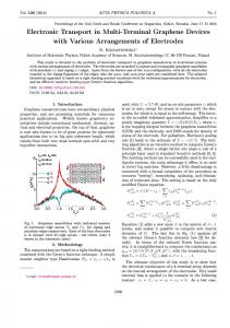
such as the ones proposed by Joshi et al. [3] and Cesnik et al. [4]. Given its tremendous potential for improving aircraft performance and for reducing costs and environmental footprint, morphing is currently the subject of widespread study, covering different aircraft components and using different materials and systems. The wing is unquestionably the major aerodynamic element of an aircraft and as such it is naturally the most obvious candidate for morphing. Over the past few decades many different designs of adaptive wings have been proposed, falling upon different parameters of the wing. Barbarino et al. [5] summarise over 150 morphing wing concepts (for both fixed wing and rotary wing applications) classified into three major categories each subdivided into specific subcategories. Figure 1.1 shows the classification of morphing strategies followed by Barbarino et al.

Figure 1.1: Categories of existing morphing wing concepts (Adapted from Barbarino et al. [5])

The main obstacle to the generalised use of such systems is their complexity. Given the size and the weight of the wing and the aerodynamic forces and moments, the implementation of successful morphing mechanisms and materials necessarily faces great challenges. Indeed, of all the morphing wing categories listed above, the only one that has been implemented in large scale with success is variable sweep, used in several fighter (e.g. F-14, Tornado, MiG-23), strike (e.g. F-111, MiG-27, Su-17, Su-24) and bomber (e.g. B-1, Tu-22M, Tu-160) aircraft. Variable sweep systems allow the wing to switch between low sweep (or even none) for optimum performance at low speeds and high sweep for operation at supersonic and high subsonic speeds. The sweep angle also has a large influence on the aircraft’s manoeuvrability and, as such, variable sweep fighter aircraft typically adapt (either automatically of through pilot control) to the particular requirements at each flight stage [6] 1 . Other morphing concepts still face 1

And since such variable sweep implementations typically consist of at most 3 different settings (take-off, landing and low speed flight; higher subsonic and/or high-g manoeuvring flight; supersonic non-manoeuvring flight) for use in distinct flight stages, it is questionable whether they fall under the definition of morphing presented above.

3

1. Introduction

technological difficulties and incur excessive penalties for the benefits and costs involved. In addition, there is a flip side to the huge role of the wing: if on the one hand the potential gains are very large, on the other hand so are the potential consequences of system failures. Given the safety-sensitive nature of all areas of aviation (civilian and military), the resistance to the acceptance and certification of new technologies likely constitutes the greatest hindrance to the actual usage of morphing wings. It is, however, possible to significantly change the overall aerodynamic behaviour of the wing using simpler, localised changes, particularly at the wingtip. The wingtip is a crucial area of the wing since it is the region where the high pressure air beneath the wing can flow (around the wing) to the low pressure area above the wing. This vortex of air flowing from beneath the wing to above it diminishes the wing’s efficiency and poses a hazard to other aircraft in the vicinity (figure 1.2). An approach to mitigate this problem consists in introducing a physical barrier to the flow of air from beneath the wing to above it2 . Many designs of such barriers have been presented and are collectively known as wingtip devices. Figure 1.3 shows the wingtip device on an Airbus A320 family aircraft. The idea of fitting such endplates to the wings is not new or even exclusive to aviation: we shall see that similar elements exist in birds and flying mammals and the first designs of wingtip devices for aircraft date to the nineteenth century; furthermore, identical systems are applied to a variety of other aerodynamic and hydrodynamic structures. Frederick William Lanchester pioneered wingtip aerodynamics studies in the 1890s and patented an aircraft design (in 1897, before man’s first successful flight) with wingtip endplates remarkably similar to modern winglets: ”The extremities of the wings may be capped by ’planes’ arranged normally to the wing surfaces and conformably to the direction of flight, in order to minimise the lateral dissipation of the supporting wave.”[8]. In a later patent [9], Lanchester proposes a different wingtip arrangement with the outer portion of the wings sloped upwards approximately 30◦ resulting in a design that resembles modern raked wingtips (although the primary goal of Lanchester’s concept was the increase of directional stability rather than performance considerations). Research on wingtip devices continued intermittently over the following decades. The Langley Memorial Aeronautical Laboratory was the site of important ad2

An alternative approach would be to use active flow control - injecting or extracting air from the wingtip region - to counter the vortex. Active flow control systems have been proposed for many different purposes including mitigating wingtip vorticity [7] but they usually involve important weight and energy penalties and/or lose efficiency at higher speeds.

4


Figure 1.2: Wingtip vortex of an agricultural plain obtained with coloured smoke (Photograph by NASA Langley Research Center / courtesy of nasaimages.org)

Figure 1.3: Wingtip device on an Airbus A320 family aircraft

5

1. Introduction

vancements in the study of the effect of wingtip plates in the 1920s both experimentally [10] and theoretically [11]. Sighard Hoerner worked on wingtip devices at Wright-Patterson Air Force Base in the 1950s arriving at a design now known as the Hoerner tip and the first wingtip design to meet some success, being found in several glider designs (figure 1.4). Nevertheless, although Hoerner concluded that ”they can be accomplished by proper design without any disadvantages or additional expenditures in construction” he acknowledged that these wingtip devices’ ”improvements are not large”[12].

Figure 1.4: Hoerner tip on a Grob G103C glider (Photograph by Michael Pereckas, available under a Creative Commons Licence. Please refer to the Image Credits on page xviii for details)

In short, early wingtip device designs suffered essentially from either of two problems that impeded their general use: the increased profile drag offset much of the gain in induced drag; and the increase in the wingroot bending moment necessitated stronger structures with the consequent cost and weight penalty. Remarkably, already in 1925 Reid was perfectly aware of these two obstacles: ”In an effort to reduce the parasite drag of the end plates, a trapezoidal shape was used in a subsequent experiment” and ”The practicability of applying such modifications to aircraft will remain in question until more is learned of the loads which they would impose upon the wing spars.” [10] The major breakthrough for wingtip designs came in the early 1970s with the 6


comprehensive study by Richard T. Whitcomb (NASA’s prolific researcher responsible for other major developments like the area rule and the supercritical wing [13]). Based on his study, Whitcomb [14] proposed a new wingtip device (the winglet) consisting of an endplate extending mostly upward from the wingtip but also comprising a small section downward from the wing tip. Wind-tunnel tests carried out between 1974 and 1976 showed that wingtip devices can reduce induced drag by about 20% and increase the lift-to-drag ratio (L/D) by about 9%. Soon after the publication of Whitcomb’s study, Heyson et al. [15] conducted a parametric comparison of winglets (of varying characteristics) with wing extensions and concluded that ”at an identical level of root bending moment, a winglet provides a greater induced efficiency increment than does a tip extension” with the authors themselves finding their results to constitute ”in general, a sweeping confirmation, for a wide range of wing designs, of the recommendations of Whitcomb in NASA TN D-8260”. The first aircraft to feature a design based on Whitcomb’s concept (even before Whitcomb’s final results were published) was Burt Rutan’s light homebuilt Vari-eze (figure 1.5) designed in 1974. The winglets on the Vari-eze doubled as vertical stabilisers and included control surfaces for rudder control. [16]

Figure 1.5: Burt Rutan’s Vari-Eze (Photograph by Adrian Pingstone)

Three years later, in 1977, Learjet displayed its innovative Model 28 business 7

1. Introduction

jet (figure 1.6) employing the first winglets on a jet and a production aircraft. Flight tests made with and without winglets showed that the winglets increased range by about 6.5 percent and also improved directional stability. [16] The importance of computational mechanics to the successful implementation of winglets must not be overlooked: indeed, it is no coincidence that this first use of winglets on a production aircraft came in the wake (no pun intended) of advances in hardware and software that allowed ”a great deal of the structural development work performed on the Learjet 28/29 wing” to be accomplished using NASTRAN analysis [17], providing a solid understanding of the structural effects of the winglet and thus addressing Reid’s cautionary words above on the practicability of wingtip devices being contingent on greater knowledge of the loads which they impose upon the wing spars.

Figure 1.6: Learjet 28 (Photograph by NASA Langley Research Center / courtesy of nasaimages.org)

The success of the early winglet applications spurred considerable interest in winglets, leading to their widespread adoption and to extensive testing confirming their advantages: Kuhlman and Liaw [18] predicted a 12% reduction in total drag for low aspect-ratio wings; Southwest Airlines has estimated that fitting winglets to its Boeing 737 aircraft reduces fuel consumption by 2.4% to 4.0% per flight (depending on flight distance); and American Airlines has calculated that 8


fitting winglets to its Boeing 737-800 and 757-200ER aircraft leads to fuel savings of 3.2% and 3.3% respectively [19]. New wingtip device designs continue to be proposed and, in some cases, successfully tested and implemented. One common theme of modern designs is the blended winglet concept consisting of a winglet extending smoothly from the wing to eliminate the abrupt transition (and associated interference drag) found in traditional winglets. In a recent two-page advertisement in a specialist publication [20], Airbus attributes the 15% reduction in fuel burn of the A320neo (in comparison with today’s A320) in part to its blended winglet design (designated ”sharklet”) which will be fitted to around 50% of the A320 family aircraft delivered in 2013 and to all aircraft delivered from 2014. [21] This success must not distract us from the fact that most wingtip device designs still carry a penalty in terms of weight (both due to the actual winglet weight and due to the stronger structure necessitated by the increase in wing root bending moment). Indeed, Buscher ¨ et al. [22] have shown that the penalty associated with the extra weight must be taken into account when designing wingtip devices, since a wingtip device designed from a purely aerodynamic approach (e.g. so as to obtain the greatest reduction in induced drag) may not be the optimum design if the increase in drag due to the higher weight is taken into account. It is not surprising then that much research effort (e.g. Takenaka et al. [23], Ning and Kroo [24]) is devoted to optimising wingtip devices so that the costbenefit balance can be improved. The potential of such optimisations is however limited by the static nature of existing wingtip devices (fixed rigid bodies, with constant shape, area, location and orientation), which force their configuration to be a compromise between the different (and sometimes conflicting) aerodynamic and structural requirements of the various flight stages/missions. Moreover, the winglet designs must comply with geometric constraints imposed by airport terminals and maintenance facilities. Hence, the potential benefits of winglets are never fully realised by a fixed design. Morphing winglets can overcome this limitation by adapting to each flight condition’s requirements and hence improve the aircraft’s performance (speed; manoeuvrability; runway requirements; climb performance; range; endurance; fuel consumption) and/or extend its flight envelope. In the future, it may be possible to design morphing winglets for specific tasks, such as mitigating an aircraft’s wake turbulence (which would allow closer spacing of aircraft during landing and take-off, thus improving runways’ throughput), improving the wing’s dynamic characteristics (flutter behaviour) or even controlling shock wave formation and/or propagation. Furthermore, morphing winglets 9

1. Introduction

change the wing’s aerodynamic forces and moments as well as its centre of gravity and the aircraft’s overall moment of inertia. The particular subject of wake turbulence merits a more detailed reference for its significance: data from the United States National Transportation Safety Board quoted in [25] estimate that in the period between 1983 and 1993 there have been 51 accidents and incidents caused by encounters with wake turbulence, resulting in the deaths of 27 occupants and serious injuries to 8 and destroying or substantially damaging 40 aircraft. Furthermore, interest in the hazardous effects of wake turbulence was revived following the dramatic crash of American Airlines flight 587 into a residential area of Queens, New York on November 12, 2001, which claimed 265 lives and caused much anxiety among the population of New York coming only 2 months after the September 11 terrorist attacks. While wake vorticity was not the direct cause of the accident, it was the major initiating factor that led the pilot to command excessive forces on the control surfaces in the attempt to escape the wake. These control surface deflections resulted in very high aerodynamic loads to the vertical stabiliser (in excess of its design limits) ultimately leading to its catastrophic failure and the loss of control of the aircraft. [26] The danger of wakes is compounded by the fact that the vortices take several minutes to dissipate, which means that any aircraft following or crossing the path of another aircraft is at risk even if separated by a few minutes. Figure 1.7 provides a striking illustration of this phenomenon, showing the extant vortices left by an Airbus A320 landing at Oakland Airport, even though the aircraft is no longer in the field of view. And just when it would seem that wingtip device design could not possibly become any more complex, things get worse: in fact, in addition to all the phenomena already considered, aircraft design must take into account a large number of factors and constraints (including aspects apparently extraneous to aircraft performance such as airport architecture), some of which may preclude the implementation of designs that would be more efficient from a purely flight performance point of view. For instance, downward canted winglets (pointing down from the wingtip) might interfere with ground handling equipment and are generally altogether ruled out, regardless of whether they might outperform other designs. Even the lower surface on Whitcomb’s design (which included a part above the wing and a smaller part below it) was judged hazardous for ground operations on some low-wing aircraft and for this reason was left out of the winglet design on the Boeing 747-400.[16] Morphing wingtip devices can overcome this problem by 10


Figure 1.7: Wake vortices left by a landing aircraft interact with the sea (Photograph by Guinnog) (Image licenced under a Creative Commons Licence. Please refer to the Image Credits on page xviii for details)

retracting or otherwise moving the wingtip device to the most favourable configuration for ground operations (even depending on the particular requirements of each airport) and changing to the best configuration (from a flight performance perspective) when at the runway or in the air. Moreover, since wingtip vortices are an inherent by-product of lift (hence the designation lift-induced drag), they form whenever different air pressure exists on the two surfaces of a wing or plate. Clearly then, they occur in any lifting surface, not only on aircraft wings. Figure 1.8 shows the vortices released from the tips of the blades of a helicopter rotor, illustrating a different occurrence of tip vortices. This implies that wingtip devices may be beneficial to many other applications beyond conventional aircraft wings. In fact, although the balance between benefits and penalties associated with the use of wingtip devices will vary from one type of lifting surface to another (depending on geometric and operating characteristics of each surface) and may not always warrant their use, studies have shown that the aerodynamic gains associated with the use of winglets are not exclusive of 11

1. Introduction

monoplane wings and extend to other wing configurations, such as biplane [27] and saucer-shaped [28] aircraft and to other lifting surfaces on aircraft: NASA’s Shuttle Carrier Aircraft (a modified Boeing 747) exemplifies this conceptual extension, employing large endplates in the tailplane (figure 1.9).

Figure 1.8: Vortices released from the blade tips of a Bell Boeing MV-22B Osprey tiltrotor (Photograph by Zachary L. Borden, for the United States Navy)

Indeed, there is no reason to limit wingtip devices to aircraft’s fixed wings: related devices (aiming to reduce tip vortices and inspired by winglets) are also found in such diverse applications as airscrews (Hartzell Q-tip blades [29] whose tip is bent backwards 90 degrees; scimitar blades, whose aerodynamically advanced planform with progressively increasing bending, twist and sweep towards the tip result in highly curved blades dictating the manufacturing process [30]), helicopter rotors (winglet-like tips on the Sikorsky S-92 blades [31]; BERP blades with their distinctive wingtips [32]), marine screws (raked blades [33]), racing yachts (keels with winglet-inspired tips [13]) and wind turbines [34]. Existing work on adaptive wingtips represents a very small fraction of the work done on morphing wings at large [35] and has mostly focussed on the change of a single winglet parameter (the cant angle) [36, 37]. Shelton et al. [36] studied both the performance implications and the control possibilities of variable cant winglets; Bourdin et al. [38] have developed considerable work on the potential of 12


Figure 1.9: Endplates on the tailplane of NASA’s Shuttle Carrier Aircraft (SCA) (Photograph by NASA Dryden Flight Research Center / courtesy of nasaimages.org)

variable cant winglets to augment and/or replace traditional control surfaces, finding that split articulated winglets can generate multi-axis control moments which are, in some circumstances, more effective than conventional control systems. Several patents have been assigned to adaptive wingtip concepts (although it must be stressed that these are generic ideas - as is usual in patent applications, even in the interest of the assignee - without detailed analysis or quantification of the benefits): Konings and Slotnick [39] patented a variable incidence wingtip aimed at changing the airflow around the wing and thus controlling the aerodynamic loads and the stalling behaviour. Irving and Davies [40] patented a rotatable winglet (with the axis of rotation ideally at a small angle to the aircraft’s longitudinal axis, i.e. the patented design consists of a variable cant winglet) in order to control the wing root bending moment. Daude [41] had patented a rotatable winglet with the same objective, but in this case varying a different parameter of the winglet orientation: the toe angle. Guida [42] patented a different approach to reducing the wing root bending moment consisting of a controllable airflow modification device (essentially a trailing edge flap in the winglet). Allen and Breitsamter have also studied winglet trailing edge flaps but with a focus on their effect on the wake [43, 44]. 13

1. Introduction

Figure 1.10: Diverse aeronautical applications of winglet-like devices From top to bottom, left to right: (a) Hartzell Q-tip airscrew on a Piper Twin Comanche (Detail of a photograph by easylocum *) ; (b) Scimitar blades on an Airbus Military A400M (Detail of a photograph by Ronnie Macdonald *) ; (c) Rotor blades of the c Sikorsky S-92 (Detail of a photograph David Monniaux *) ; (d) BERP rotor on an AgustaWestland EH101 (Detail of a photograph by Jerry Gunner *) (* Images licenced under Creative Commons Licences. Please refer to the Image Credits on page xviii for details)

14


Figure 1.11: Applications of winglet-like devices in other fields Left: Winglet on a wind turbine rotor (Photograph by TraceyR *) ; Right: Endplates on the wings (front and rear) of a McLaren MP4/4 Formula 1 car (Photograph by Norimasa Hayashida *) (* Images licenced under Creative Commons Licences. Please refer to the Image Credits on page xviii for details)

The most advanced and promising adaptive wingtip device design developed thus far is the MORPHLET project [45], consisting of a four partition winglet able to vary the dihedral (cant), twist, taper and span of each partition individually. It is, however, a complex design that also relies heavily upon further developments in innovative materials and systems. Is there another way to tackle the adaptive wingtip device problem? And if so, will it yield better results? The core subject of this thesis is thus the study of the influence of the various wingtip device parameters on the overall wing behaviour while searching for a simple adaptive wingtip device concept (involving as few parts - particularly moving parts - as possible, for high reliability, low weight and low cost) relying solely on available (or soon to become available) technologies. This brief overview of morphing and the importance of wingtip aerodynamics would not be complete without a reference to the XB-70 Valkyrie: developed by North American Aviation in the late 1950s as a high-altitude, supersonic (Mach 3), long range (6000 nautical miles) bomber able to operate from conventional runways, it was a fascinating and inherently complex design incorporating many innovative features. One of the these was the ability to droop the wing tips, changing the orientation of the outer portion of the wing from straight with the central portion of the wing (at low speeds) to 25◦ tip down (at transonic speeds) and ultimately 65◦ tip down (at supersonic speeds)[46]. Figure 1.12 shows the Valkyrie in flight with the three different wingtip configurations. The benefits of the drooped wingtips in supersonic flight were twofold: improvement in directional stability and 15

1. Introduction

increase in the lift-to-drag ratio by taking advantage of compression lift [47]. The latter is an aerodynamic phenomenon described by Eggers and Syvertson [48] in 1956 where adequately shaped aircraft can ride their own shock waves generating extra lift. While it can’t be regarded as an actual adaptive wingtip device design in the modern sense (work on wingtip devices only began in earnest several years later, and the drooping wing tips of the XB-70 represent over one third of the wing half-span, much more than traditional wingtip devices - leading Barbarino et al. [5] to classify it as ”span bending” rather than an adaptive wingtip device) this is nevertheless a very interesting example of the possibilities associated with variable-orientation wingtips and for how long there has been awareness of such potential. Indeed, the drooping wing tips of the Valkyrie are instrumental to the realisation of compression lift, which was the principal factor behind the unanimous selection of Northern American Aviation’s design by the United States Air Force’s selection team [49, 50]. The Valkyrie’s mechanism also provides the best (or at any rate, the most graphic) illustration of the enormous influence of wingtip aerodynamics and the magnitude of the impact of changes in wingtip devices: without the drooping wingtips (and thus the increased lift-to-drag from the usage of compression lift), the only way to meet the required range was North American’s initial design involving the use of jettisonable external fuel tanks (mounted on the wingtips) of such huge dimension that General LeMay’s reaction on seeing such ”monstrosity” was: ”This isn’t an airplane, it’s a three-plane formation.” [49, 51] Finally, the fact that this design too (at a different time and with different objectives from today’s morphing efforts) focussed solely on varying the cant angle is a striking testimony of the immense importance of this variable and of the enormous influence of the wingtip’s cant angle in the overall wing aerodynamics.3

1.2 Biomimetics: learning from nature’s flying machines The first known bird, Archaeopteryx, flew over the Earth about 150 million years ago, culminating an evolutionary process that gave animals the ability to fly and beginning another evolutionary process that saw enormous improvements in avian flight performance.[52] The morphology of contemporary birds embod3

Incidentally, a fatal accident involving one of the two XB-70 Valkyrie prototypes (believed to have been caused or exacerbated by the Valkyrie’s wingtip vortex wake) was a major driving force in the study of wake vortices and wingtip aerodynamics which, in turn, contributed to the development of modern wingtip devices.

16

1.2 Biomimetics: learning from nature’s flying machines

Figure 1.12: Drooping wingtips on the North American XB-70 Valkyrie Standard position (top) ; Drooped to 25◦ (centre) ; Drooped to 65◦ (bottom) (Photographs by NASA Dryden Flight Research Center / courtesy of nasaimages.org)

17

1. Introduction

ies the results of this evolution and constitutes an immense body of knowledge upon which engineers can and have inspired themselves when looking for ways to improve aircraft. ”For years engineers have recognised that when they hit a problem, nature has probably encountered and resolved that same issue years before. It’s a sensible place to start looking for a solution.” [53] Still in Kay’s words: ”Take the solution to managing airflow in and around the jet engine - a repetition from nature” - just as a wall of air would build in front of a peregrine falcon diving at over 300 km/h preventing it from breathing so would a plain engine intake at high speed constitute a wall for incoming flow, deflecting the air around the engine and preventing its regular breathing thus compromising the engine’s combustion and ultimately stalling it. And just as peregrine falcons have cone-shaped bones protruding from the nares to control the flow of incoming air, so have engineers devised engine intakes with protruding cones to manage the airflow and ensure proper engine breathing. [54] Figure 1.13 shows the similarity between the cone in the peregrine falcon’s nares and the engine intake on a Mikoyan-Gurevich MiG-21.

Figure 1.13: Nature inspires technology: peregrine falcon’s nares and jet engine intake on a MiG-21 Left: Cone on the nare of a peregrine falcon (Photograph by Greg Hume *) ; Right: Mikoyan-Gurevich MiG-21 with the engine intake cone (green) clearly visible in the foreground (Detail of a photograph by the United States Air Force) (* Image licenced under a Creative Commons Licence. Please refer to the Image Credits on page xviii for details)

The very idea of morphing is inspired by avian flight: birds are not static machines that remain unchanged throughout and between flights; rather, they permanently and continuously adapt to the prevailing conditions by changing their morphology. In Hanson’s words: ”If you have ever flown in a window seat, you 18


may have admired the silvery shine of an airplane wing and watched its several flaps raise and lower at various times during the flight. It’s a precise and beautifully designed instrument, but must look terribly crude to a bird, whose own wings can flap and flex, extend and contract, spread, narrow, tuck and twist, responding instantly to ever-changing conditions.”[55] Wingtip devices, too, are an adaptation of features found in birds’ (and other flying animals’) wings [56], mimicking different approaches found in nature - ranging from the Flying Squirrel’s ability to extend the tip of the wing upwards by means of a cartilage at the wrist to produce a winglet-like surface [57] to the capability to spread the primary feathers at the wingtips thus creating very large slots between the individual feathers, which is typical of many medium and largesized birds such as the California Condor [58]. Figure 1.14 shows the slotted wingtip feathers on a Yellow-legged Gull. This difference in the anatomy and aerodynamics of the wingtips of flying animals with diverse flight regimes and requirements is remarkable and suggests that there is no such thing as a perfect wingtip configuration but rather that the ideal wingtip design depends on the operating conditions. Bushnell and Moore [59] provide an extensive review of drag reduction mechanisms found in nature, dedicating two pages specifically to the reduction of drag due to lift. In addition to the avian-inspired techniques discussed above, the authors also present several avenues of research based on underwater creatures, namely: ”(a) swept-back tapered tips (which also occur on birds); (b) serrated trailing edges, both local near the tip (shark) and along the entire trailing edge (humpback whale, also many birds) ; (c) leading-edge bumps (pectoral fin on humpback whale, head on hammerhead shark); and (d) ’fin rays’ or wavy flowaligned surface relief, including the optimal alignment of denticles near the tip.” Given this ubiquity of wingtip devices and similar designs in nature, it comes as no surprise that here too natural evolution foreshadowed mankind’s technological approach: indeed, Richard T. Whitcomb’s inspiration for his ground breaking work on winglets (which eventually led to their widespread adoption) came from an article in Science magazine about the use of tip feathers in soaring birds [60]. And whereas Whitcomb’s and most subsequent designs took inspiration from nature but evolved into more practical geometries than the split wingtip feathers found in birds, many designs of ”multiple winglets” (closely resembling birds’ split feathers) have been studied. [36, 61, 62] The major problem with this concept is that, while a greater number of individual winglets leads to larger reductions in induced drag, this improvement comes at the cost of increased interference 19

1. Introduction

Figure 1.14: Slotted wingtip feathers on a seagull

and larger friction drag. [63] A solution to this problem lies in spiroid wingtips proposed independently by different researchers [63, 64] and constituting a hybrid of sorts of Whitcomb’s single winglet and nature’s multiple split feathers: the spiroid wingtip is simply a split-wing loop extending from the tip of the wing (figure 1.15) and combining the optimal vorticity distribution of multiple winglets with the simplicity and absence of interference of single winglets. More importantly, however, while each of these man-made versions (sophisticated as they may be) have hitherto been merely static devices, the wingtips of birds change throughout the flight in order to adapt to the conditions and requirements of each moment. Again, quoting Hanson: ”Vultures, eagles, and other soaring birds use small adjustments of their spread wing-tip ’fingers’ to manipulate air currents or change speed and orientation, and all birds utilize feather movements to instinctively alter the turbulence patterns around their wings.” [55] The pioneers of bird flight study were aware of (or should we rather say sensed) the importance of the wingtip in the overall wing aerodynamics, and devoted some of their time and work to the analysis of the aerodynamic behaviour of wingtips. Leonardo da Vinci explicitly addresses the role of the wingtips (particularly in terms of flight stability and control) in different folios of the ”Codex on the Flight of Birds” [65]. Figure 1.16 illustrates one of these thoughts of Leonardo, 20


Figure 1.15: Spiroid winglet on a Dassault Falcon 50 (Photograph by FlugKerl2) (Image licenced under a Creative Commons Licence. Please refer to the Image Credits on page xviii for details)

describing how a bird can counter lateral winds by folding the wingtip. Otto Lilienthal also devotes part of his ”Birdflight as the Basis of Aviation” to the influence of the wingtips on the aerodynamics of birds. In particular, he concludes that the effect of the wingtips (and their varying orientation) is not so much the generation of lift but rather the production of thrust [66]. While Lilienthal’s study dealt with the aerodynamics of flapping flight (and his analysis of the influence of the wingtips - taking into account the different wingtip orientation between the upstroke and the downstroke - is specific to flapping flight), his conclusion is also valid - albeit in a slightly different way - in the case of fixed wing flight: the finite wing penalty translates mostly into increased drag and only in a minor scale into decreased lift. Thus, the main effect of winglets and other wingtip devices on aircraft is a reduction in drag and only secondarily an increase in lift, paralleling the effect observed by Lilienthal in birds. Figure 1.17 illustrates the position of the various wing parts throughout one flapping cycle. Notice how the two wings on the bottom right of the plate (the one on the left representing the wing configuration during the downstroke and the one on the right the wing configuration during the upstroke) have wingtips with significantly different orientations. But perhaps the most important lesson nature can teach us as regards wingtip 21

1. Introduction

Figure 1.16: Wingtip deflection in a bird to counter lateral winds (Detail of folio 8r from the ”Codex on the Flight of Birds”, by Leonardo da Vinci)

aerodynamics is the fact that different flight requirements prompt different wingtip arrangements. Lazos [67] describes the differences in the wing planforms of the Wandering Albatross, typical of soaring seabirds, and of the California Condor, typical of soaring landbirds. Particularly, it is seen that the former has a sharp swept tip whereas the latter have splayed feathers at the tip. The fact that millions of years of evolution have resulted in such distinct configurations for birds with different flight conditions is a stark reminder that there is no such thing as a single wingtip-fits-all design. This constitutes the ultimate motivation for the development of adaptive wingtip devices capable of tailoring their configuration to the prevailing conditions and requirements.

1.3 Thesis objectives, outline and contributions From what has been said above, it is clear by now that the main goal of this thesis is the study of adaptive wingtips for aircraft wings and the definition of a suitable concept, including the quantification of the benefits and penalties of such a concept compared to conventional fixed wingtip devices. The first step in this endeavour is the analysis of existing (or in advanced stages of development) materials and systems suitable for application to the design of adaptive wingtips. Chapter 2 presents this review, focussing in the detailed study and comparison of the most promising approaches: the use of multistable composites; and the use of hinge mechanisms analogous to the ones used on current aircraft control surfaces, flaps, and other moving surfaces. The latter is seen to be a more mature technology and its advantages outweigh its disadvantages. Given the enormous variety of aircraft of wildly different configurations and dimensions, it is important to assess how the performance and cost of any proposed system vary relative to the aircraft type and weight. The chapter therefore closes with some thoughts on the scalability of the envisaged adaptive wingtip 22

1.3 Thesis objectives, outline and contributions

Figure 1.17: Change in wing and wingtip orientation of the stork throughout the flapping cycle (Plate 8 from the German first edition of Otto Lilienthal’s ”Birdflight as the Basis of Aviation”)

mechanism. Chapter 3 presents the design work conducing to a preliminary adaptive winglet (applying the mechanism defined in the previous chapter to a basic winglet with rectangular planar form, average spanwise length and symmetric aerofoil) and presents the computational model used to evaluate its performance (both in aerodynamic and structural terms) and to compare it with that of an ideal fixed wingtip device. This computational model forms the core of an optimisation procedure that yields the best configuration of the proposed design for different flight conditions. The results illustrate the different winglet configurations for the various flight conditions and explore the physics underpinning those configurations. The chapter then describes the construction of a prototype of the proposed design and the results of its testing (centred on the actuator’s capabilities and on the overall system’s dynamic behaviour), confirming the feasibility of the concept. Chapter 4 extends the analysis to study the performance of the proposed variable-orientation winglet in the case of more generic wingtip devices of varied 23

1. Introduction

length, planform, aerofoil and shape (including torsion and bending). The new, extended, computational model is presented as are more advanced optimisation algorithms prompted by the greater complexity (and increased non-linearities) of the new model. Given the extended model’s ability to study wingtip devices of highly varied geometries, an assessment of the potential gains obtainable with an hypothetical wingtip device able to vary all the considered geometric parameters is also conducted. The results compare the performance of a fixed winglet with those of two different embodiments of the proposed variable orientation winglet (variable toe and cant; variable toe, cant and sweep) and with those of the hypothetical wingtip device able to change each and all of its characteristics. In the latter case, attention is given to which of the wingtip’s geometric parameters have a greater influence in its performance, providing an important lead for the future research of wingtip devices with greater morphing capabilities. Finally, chapter 5 summarises the work presented throughout the thesis and its most important results, as well as establishing and laying the groundwork for future developments in this area. The main contributions of this thesis to the state of the art in adaptive aircraft systems are also enumerated. Considering that one of the primary purposes of a thesis is the dissemination of novel findings, this introduction would not be complete without a few words about the original contributions stemming from the present work. Clearly, the central contribution of this thesis to the state of the art in the field of aerospace engineering is the design of an adaptive wingtip device able to outperform fixed winglets and a complete evaluation of its performance. At the same time, the design and implementation of an innovative concept such as this is not a straightforward task and will require the development of new tools and techniques to support it. While ancillary to the main goal of this thesis, such tools and techniques (encompassing different disciplines such as materials engineering and computational methods) can constitute valuable developments with application to this and different areas of research and will therefore also be highlighted. These include: a dynamic thermo-structural finite element model of multistable composites and a comparison of the results obtained with this model and with the common purely structural models; a design method (inverse problem) for multistable composites that determines the composite plate’s configuration leading to the shapes most closely resembling those specified by the user; an automated fluid-structure interaction analysis procedure allowing coupled field analyses using ANSYS and CFX to be run without any user intervention and thus suitable for inclusion in such batch executions as optimisation procedures, sensitivity analyses or regression 24

1.3 Thesis objectives, outline and contributions

building; a multi-fidelity polynomial regression algorithm allowing the obtention (with an excellent balance between accuracy and computational cost) of polynomial approximations for any quantities estimated numerically, and an application of this algorithm to the construction of polynomial approximations of the lift and drag coefficients for a wing with an adaptive wingtip device; a systematic analysis of the effects of 11 major wingtip device geometry parameters (including the combined effects of changing various parameters) on the aerodynamic behaviour of the wing, thus greatly extending the studies currently found in the literature. In the expectation that these contributions will prove useful and constitute building blocks (small as they may be) of many future advancements, I invite you to explore this thesis and hope you enjoy reading it as much as I enjoyed writing it.

25

1. Introduction

26

2 Enabling technologies The previous chapter set out the motivation of this work and established as the main goal the design and study of an adaptive wingtip device for aircraft. The present chapter reviews the state of the art in adaptive aircraft systems in order to determine the most suitable materials and technologies to implement an adaptive wingtip device. Such materials and technologies can be grouped into two broad categories: novel structures and actuators; and conventional structures and actuators. The former comprise the so-called smart materials, which take advantage of physical properties which until recently were either unknown or considered of no practical interest. Examples include: materials with negative Poisson’s ratio (which, when stretched in the axial direction, will also stretch in the transverse directions, rather than compressing); magnetorheological and electrorheological materials (whose viscosity is a function of the applied magnetic or electric field, respectively); piezoelectric materials (which deform in response to an electric field and vice-versa); shape-memory alloys (which will revert to one or more predefined shapes when certain temperatures are applied) and multistable materials (having more than one stable shape and the ability to reversibly change between these shapes when an adequate load is applied). The latter comprise the alloys and composites which have been in widespread use for the past few decades as well as electric, hydraulic and pneumatic actuators (both linear and rotary, in an enormous variety of designs) also commonly 27

2. Enabling technologies

found in aircraft. Novel technologies generally present some advantages in terms of functionality and effectiveness but are often limited to niche applications as the underlying technologies are not yet fully mature; conventional systems, on the other hand, are highly efficient (the product of continuous development over long periods of time), proven and reliable (two key aspects in terms of regulatory and industrial acceptance). In short, except for highly specific scenarios that may altogether require the use of one or the other class of materials and systems, it is generally not possible to say a priori that one of these technological avenues is better. This chapter will therefore consider materials and systems pertaining to both groups. Prior to the analysis of the candidate technologies conducing to the selection of the most appealing solution, it is first necessary to establish how is the wingtip device’s adaptability going to be implemented. What parameters are going to be varied? Within which intervals? How often throughout the flight? Only after answering these questions will it be possible to have a clear vision of the desired solution and only then can the adequacy of the various technologies be assessed. Takenaka et al. [23] have determined that the major influences to the various components of drag and to the wingroot bending moment come from the cant and toe angles and the winglet span length as well as to correlations of these. In particular, the toe angle shows great promise for morphing, since it is only optimum for one flight condition. This is because the toe angle controls the overall loading on the winglet as well as its effect on the load distribution of the whole wing and, simultaneously, the angle of attack of the winglet is a function of the wing’s lift coefficient, which depends on the flight condition. For this reason, the toe angle in a fixed wingtip is a compromise that attempts to maximise the wing’s performance over the entire flight envelope [68]. Specifically, greater toe angles are associated with better climb performance at the cost of high-speed performance [69]. Figure 2.1 illustrates the winglet cant and toe angles, with the rotations performed in sequence (i.e., the coordinate frame is first rotated about the cant axis - parallel to the aircraft’s longitudinal axis - and the resulting, rotated, coordinate frame is, in turn, rotated about the toe axis - parallel to the winglet’s span). The sign conventions are those most commonly found in the literature: • The cant angle is measured outwards from an upward vertical (i.e. a perfectly vertical winglet pointing upwards has 0◦ cant; a ”winglet” aligned with the wing - essentially a wing extension - has 90◦ cant; and a perfectly vertical winglet pointing downwards has 180◦ cant.) 28

• The toe angle is measured inward from an axis parallel to the aircraft’s longitudinal axis (i.e. toe-in corresponds to positive toe angles; and toe-out to negative toe angles)

Figure 2.1: Illustration of the winglet’s cant and toe angles

Clearly then, the candidate parameters to be varied in the adaptive wingtip device design are the cant angle, the toe angle and the wingtip device’s spanwise length. In addition to Takenaka et al. [23], Heyson et al. [15] also analysed the effect of various parameters (including the cant and toe angles and the spanwise length) on the wing performance and root bending moment. Specifically, Heyson et al. concluded that: – The toe angle ”provides design freedom to trade small reductions in induced efficiency increment for large percentage reductions in the root bending moment increment”. This suggests an obvious morphing application: a fixed winglet has a toe angle that balances the desire for greater efficiency with the need to maintain the root bending moment moderate to avoid the need for an excessively strong (and heavy) structure. A variable toe winglet, on the other hand, can adopt the toe angle producing the lowest root bending moment when the aircraft is operating in conditions near its maximum design bending moment and change to the toe angle associated with the highest efficiency when operating in conditions significantly below the wing’s structural limits. It is also seen that the optimum toe angle depends on other parameters such as the wing’s aspect ratio, taper and washout (twist), implying that if a variable toe winglet is applied to a morphing wing able to vary 29


either of those parameters the control algorithm responsible for the determination of the ideal toe angle must take all those variables into account. – ”Both induced efficiency and root bending moment increase continuously as the winglet is canted further outward”. Again, the relation between efficiency and wing root bending moment is present, highlighting the potential for performance gains if the winglet is able to adapt the cant angle in response to the prevailing conditions and flight profile. Heyson et al. further found that for winglets of coeval design ”the greatest advantage relative to a tip extension is obtained for nearly vertical winglets”. While this observation was made for the winglet designs of the time, most designs of winglets up to the present time seem to confirm it being, as they are, nearly vertical. It is, however, necessary to emphasise that the above conclusion is specific to efficiency, which means that there is here another even more promising, if surreptitious, case for morphing: since aircraft are usually designed with efficiency in mind, the typical winglet designs assume the most efficient configuration. Yet, efficiency is not always the main objective: when taking off or landing (particularly in short runways) other considerations come to the forefront - in these cases it is often preferable to operate less efficiently for the short duration of the take-off or landing in exchange for the ability to operate safely from runways that might otherwise be outside the aircraft’s capabilities. In other words, whereas an aircraft designed for maximum efficiency must necessarily forgo operating in short runways (and, conversely, aircraft designed for short take-off and landing - STOL - operations generally have such capability at the expense of cruising efficiency), an aircraft with a variable cant angle winglet can adopt the configuration producing the most lift for STOL operations, then change to the most efficient configuration for cruise. – ”Both induced efficiency and root bending moment increase with winglet length” but with the moment increasing more rapidly than the efficiency. This means that, although once again we find the same opportunity for trading root bending moment for efficiency according to each moment’s prevailing conditions, that possibility is less attractive here since it it will lead to a disproportionate penalty. These findings suggest that there is significant potential in the ability to change the winglet’s cant and toe angles and, to a lesser degree, its length. At the same time, it is important to keep in mind that the adaptive wingtip design needs to 30

combine conflicting aspects: it must be simple (comprising few and uncomplicated parts) in order to maximise robustness and reliability and minimise costs (both initial and operating) and to ease as much as possible the certification and acceptance of this new concept; while simultaneously it must be as effective as possible in order to warrant its implementation and highlight its benefits. This means that the potential for gains associated with the variation of each parameter must be compared to the complexity, weight and cost involved in its actuation. And here, an important distinction among the three parameters (cant, toe, length) arises: whereas the cant and toe angles, expressing the winglet’s orientation relative to the wing, can be changed simply by rotating the whole winglet about the tip of the wing, a variation in the winglet’s length requires much more complex mechanisms, such as a telescoping winglet. While telescoping wings have been proposed and built, they involve larger costs and difficulties that have so far impeded their widespread adoption. Indeed, it is certainly not a coincidence that, as noted in chapter 1, the only very successful wing morphing capability to date is the variable sweep wing which consists solely in the rotation of the wing about an axis at its root. One can surmise that the variable sweep mechanism’s simplicity1 played an important part in its successful implementation. Designing a winglet with the ability to simultaneously (and independently) vary the cant and the toe angles will necessarily involve one step forward in terms of weight and complexity of the mechanism when compared to the variable sweep wing but still a clearly feasible mechanism not entailing excessive penalties, it is reckoned. Hence, while the computational models to be implemented in this thesis for the analysis of adaptive wingtip devices may be used to evaluate the effects of changing other parameters, the central focus of this thesis will be the design and study of a wingtip device with variable cant and toe. Now that a general view of the intended adaptive wingtip device concept has been formed, it is necessary to determine the most suitable technologies to implement it. This process naturally begins with a review of the technologies adopted by other adaptive aircraft components. Sofla et al. [1] and Barbarino et al. [5] reviewed over one hundred concepts with largely different materials and actuators. One trend that is apparent when considering these concepts is the widespread usage of smart materials in applications requiring low actuation energy (such as camber variation) but the almost universal preference for conventional actuators in applications requiring large displacement and/or force. This is in keeping with 1

A fundamental aspect of this simplicity in terms of keeping the size and weight of the mechanism in check as well as ensuring its reliability is the very low number of moving parts.

31


the, as yet, limited energy actuation capabilities of most smart materials. Among the individual technologies used in morphing systems, the most common are Shape Memory Alloys (SMAs), Piezoelectrics (PZTs), electric motors (including servos), pneumatic and hydraulic actuators. In addition, there has been interest in the application of multistable composites to morphing aircraft structures, given these materials’ attractive properties (described in greater detail below). [70] This chapter will therefore present a closer look at these candidate technologies. In keeping with the classification introduced above, this study will be divided into two different sections: the first dealing with novel materials (namely multistable composites actuated by shape memory alloys or piezoelectrics); the second considering conventional actuators (namely electric motors and hydraulic and pneumatic actuators). These studies will be followed by an assessment of the most suitable technology for application to adaptive wingtip devices of the type presented above (variable cant and toe angles) at this time.

2.1 Multistable composites controlled by novel actuators Multistable structures are those than can have different shapes and which will retain either shape until they are forced to change (typically by applying an external load), i.e., energy is only required to change the structure from one shape to another but not to keep the newly acquired shape. Even though other solutions have been proposed (Kebadze et al. [71] describe a multistable plate made up of several half-circular strips of beryllium-copper), multistable composites consisting of laminated plates of fibre-reinforced plastics are the subject of great interest due to a combination of properties (most importantly very good strength to weight ratio) that make composites in general an ideal material for aerospace applications. Orthotropic composites (such as carbon fibre + epoxy or glass fibre + epoxy) have different coefficients of thermal expansion αi along different directions. Hence, when such a material is subjected to a temperature difference, it will experience different strains ǫi along each direction i in accordance with: ǫi = αi × ∆T

(2.1)

If several layers of such a material are stacked with different fibre orientations and cured together, once they are cooled down to room temperature the various layers will tend to have different strains. Since the various layers are bonded 32

2.1 Multistable composites controlled by novel actuators

and cannot freely stretch relative to each other, the plate will develop a curvature that best accommodates the conflicting individual strains and that minimises the residual stresses associated with the inability of each layer to freely stretch by the amount given by eq. 2.1. This curvature (forming a saddle shape) is illustrated in figure 2.2.

Figure 2.2: Saddle shape of a multistable composite combining two conflicting curvatures As the cooling process progresses and the temperature change (relative to the curing temperature) increases, the magnitude of the plate’s curvature also increases. If the temperature change exceeds a certain threshold (which depends on the plate’s shape, dimensions, material and layer stacking sequence), there is no curvature of the plate that can accommodate the conflicting thermal strains of the various layers. When this happens, the influence of one of these conflicting thermal strains prevails (which one will prevail is determined by manufacturing and/or environmental constraints) and the plate acquires a curvature dominated by the thermal strains of one of the layers (fig. 2.3, left). However, significant residual stresses will be present (associated with the thermal strains of the other 33


layer(s)) and if an appropriate load (generally referred to as the snap-through force) is applied to the plate, it will acquire a curvature dominated by the thermal strains of those other layers (fig. 2.3, right).

Figure 2.3: Stable shapes of a square multistable composite plate fixed at its centre The key feature of multistable composites lays in the fact that this curvature will remain even after the load is removed. Either curvature is therefore stable and the plate’s shape can be switched back and forth between both curvatures as many times as desired by applying an appropriate load. Suitable actuators include shape-memory alloys (SMA) [72] and macro fibre composite (MFC) piezoelectric actuators [73]. Multistable composites are promising candidates for morphing wingtips since they are able to change shape without the need for permanent actuation (energy is only spent when changing from one shape to another; maintaining either shape requires no energy) and can withstand significant loads. One limitation of multistable composites is the fact that the number of stable shapes is limited - most multistable composites can only switch between 2 different shapes. If several multistable composites are combined, the total number of shapes is dictated by the combinations of shapes of individual composites. This increases the complexity (particularly in terms of the design of the actuation system to change from one shape to another) but makes for a significantly more powerful system. The number of shapes is, however, still finite which makes systems based on multistable composites more suitable for components where different discrete configurations are needed than for systems where a smooth, continuous movement is required (as in control surfaces). Multistable composites have significant advantages: 34


• Low weight • Actuation is only required for the snap-through, i.e., only during the shape change. No energy is required to maintain either shape • Being made of materials with very good stiffness and strength, multistable composites do not need a separate structure and can combine structure and morphing mechanism in a single component • Furthermore, since composites (both multistable and conventional) can be made to virtually any shape, they may be used as monocoque components: combining structure and skin in the same component However they also have important drawbacks: • Even though the term ”multistable composites” is generally used, most are actually ”bistable composites”, i.e., they can only switch between two different shapes. This reduces their adaptability and, in particular, seriously limits their use as control surface replacements or augmentation devices • Size: composite plates (even when built as described above) only exhibit multistable behaviour if the ratio of the in-plane dimensions to the thickness exceeds a certain critical threshold (dependant on the material, geometry and curing temperature). Since the thickness cannot be reduced beyond a certain point (dictated by the thickness of each composite layer and the number of layers), this forces the in-plane dimensions to be above values of the order of 5cm for a typical plate • Possibility of uncommanded snap-through: if the plate is subjected to a load greater than its snap-through force, it can change shape undesirably with potentially adverse consequences • High cost • Slow construction of each individual component (in comparison to e.g. the manufacture of metallic components by sheet stamping) although in the case of larger and more complex geometries this competitive disadvantage is made up for by the possibility of creating one single composite component as opposed to the need to manufacture and assemble different metallic parts 35


Various concepts are analysed to explore the multistable composites’ advantages while minimising the effects of their disadvantages. The major drawback is the limitation of each plate to only 2 different shapes. This can however be circumvented by combining various plates, as discussed in greater detail in the following section. The simplest multistable composite plates are square plates made up of two layers of a composite material of resin and unidirectional fibres, with one layer’s fibres perpendicular to the other layer’s fibres (e.g. a [0,90] stacking sequence), fixed in the centre, and these have been object of study for some time (e.g. [74],[75]). However the shapes obtained with such plates (shown in figure 2.3 two curvatures about different axes) are of little interest for application to wingtips. This prompts the need to devise different multistable composite plate designs (different geometry, stacking sequence and/or constraint). Rectangular plates comprising two regions (one with a symmetric composite stacking sequence and another with an unsymmetric stacking sequence) have been proposed [70] to allow shapes of greater practical interest. Although the multistable behaviour is only associated with unsymmetric stacking sequences, the presence of a region with symmetric stacking constrains the plate and influences the overall stable shapes. Such plates will essentially bend along a single direction when snapped-through from a stable shape to another. The geometry of one such plate is shown in fig. 2.4 (above), along with the stacking sequence of both regions (below). An alternative approach is to use a square plate fixed along one of its edges (rather than at the centre). The shapes of one such plate are shown in fig. 2.5.

2.1.1

Multistable composite plate modelling

Theoretical approaches to the design of components based on multistable composites are hampered by their non-linear behaviour (both during the manufacture of the composite and during the change from one stable shape to another - the ”snap-through”). Furthermore, the geometries of interest from an engineering standpoint need not be regular shapes. Thus, while theoretical models of the behaviour of multistable composite plates have been employed with success for problems involving simple regular geometries, the generic analysis of more complex plates requires the use of finite element modelling (FEM) [76, 77]. FEM is an ubiquitous, well-tested tool for the analysis of mechanical components and can easily be integrated in a design optimisation procedure. Composite material 36


Figure 2.4: Geometry and stacking sequences of a rectangular multistable plate

Figure 2.5: Stable shapes of a square multistable composite plate fixed along one edge

37


models and elements with non-linear formulation are required for the analysis of multistable composites. If a finite element program with computational fluid dynamics (CFD) capabilities is used, a multidisciplinary analysis of the multistable composite plate can be carried out, combining aerodynamic and structural effects. The ANSYS finite element suite meets all these requirements and was therefore used in the course of this work. The mechanical properties of unidirectional carbon fibre/epoxy composites used in the analysis are shown in table 2.1. Table 2.1: Mechanical properties of carbon fibre/epoxy composites Property Young’s modulus along fibre direction Young’s modulus normal to fibre direction Shear modulus in fibre planes Shear modulus in plane normal to fibres Poisson’s ratio in fibre planes Poisson’s ratio in plane normal to fibres Thermal expansion coefficient in fibre direction Thermal expansion coefficient normal to fibre direction Density

Value 20 msi 1.3 msi 1.03 msi 0.90 msi 0.3 0.49 1.0 10−6 /◦ F 30.0 10−6 /◦ F 1600 kg/m3

Source [78] [78] [78] [78] [78] [78] [78] [78] [79]

msi = million psi (1msi = 6.895 × 109 P a); 1/◦ F = 1.8/K

It is important to note that in a square plate the unstable saddle shape shown in figure 2.2 (combining the conflicting curvatures imposed by the various layers), although not found in the physical world for values of ∆T (temperature change relative to the curing temperature) above the threshold described in the previous section, is a mathematical solution to the problem. When analysing an ideal square plate (with equal length along both directions) and without any asymmetries, the finite element analysis converges to the saddle shape. To take into account the asymmetries that inevitably exist in actual plates (be it in the geometry or the material, which unlike in numerical analysis, can never be perfectly homogeneous in reality) and lead to the bistable shapes, some sort of imperfection must be introduced in the numerical model. This can be accomplished by simulating the square plate with a rectangular plate with nearly equal sides [80]. The cool-down process is simulated by setting the initial temperature to the composite’s curing temperature and then lowering the temperature (to its normal operating temperature). To facilitate convergence, the plate can be cooled down in small increments at a time. 38


The computational models of multistable composites presented in the literature ([77, 80–82]) simulate the cooling by applying the desired temperature uniformly throughout the plate. This neglects the thermodynamics of the cooling process. Even though the multistable plates are usually thin (and hence it is not expected that large temperature gradients will develop within the plate), it is important to determine the effects of the actual cooling process by modelling the heat transfer process as it occurs in reality. This requires the solution of the equations of thermodynamics (in addition to the structural ones) and the definition of the thermal material properties and boundary conditions. Table 2.2 presents the thermal properties of carbon fibre/epoxy composites. Table 2.2: Thermal properties of carbon fibre/epoxy composites Property Value Source Thermal conductivity along fibre direction 5 W/m.K [83] Thermal conductivity normal to fibre direction 0.5 W/m.K [83] Specific heat 1000 J/m.K [84]

The boundary conditions are defined assuming forced convection (with a fan or other system forcing air circulation around the plate to cool it)2 based on the equations found in [85]. For the typical multistable plate dimensions and cooling air flow velocity, the flow is entirely laminar and the average Nusselt number is given by: ¯ L = 0.664Re1/2 P r 1/3 Nu L

(2.2)

The average convection coefficient is then obtained according to: ¯ ¯ = NuL k h L

(2.3)

Based on the above equations and on the air properties presented in [85], it is now possible to calculate the average convection coefficient. Since the properties of air are a function of temperature, it is necessary to determine and compare the convection coefficient at different ambient temperatures. Assuming a convection air flow with a velocity of 15 m/s and a plate with a reference length of 15 cm, the various parameters (and ultimately the average 2

Note that the finite element model can use any other cooling method such as natural convection, conduction or radiation, with the only required change being the specification of the appropriate parameters.

39

2. Enabling technologies convection coefficient) at ambient temperatures of 300 K and 450 K (approximately corresponding respectively to the final operating temperature of the plate and the initial curing temperature) are:

T [K] 300 450

Table 2.3: Convection parameters 2 ¯ ¯ ν[m /s] k[W/m.K] Pr Re Nu h[W/m K] 1.59e-5 2.63e-2 0.707 4.72e4 129 22.5 3.24e-5 3.73e-2 0.686 2.32e4 89.1 22.2 2

Given the small difference in the average convection coefficient between the initial and final temperatures, it was decided to use a constant value of 22.5 W/m2 K throughout the cooling process rather than interpolating the value based on the temperature at each moment in the cooling process. Figure 2.6 compares the plate shapes after cooling completion obtained with both approaches (solution of the heat transfer equations on the left; uniform temperature imposed throughout the plate on the right). Figure 2.7 is analogous but for the plate shapes after snap-through. Table 2.4 lists the maximum deflection value in each case. It is evident from both figures and from the table that the differences between both models are negligible (with the difference in the maximum deflection value being less than 0.01% in the post-cooling shape and 0.76% in the post-snap-through shape). These results confirm the validity of the approach commonly found in the literature and consisting of imposing a uniform temperature throughout the plate. This, in addition to the large increase in computation time required by the solution of the heat transfer equations, dictates the usage in the remainder of this thesis of the usual cooling model (uniform temperature) instead of the inclusion of the thermodynamic physics. Table 2.4: Maximum deflection magnitude for multistable composite plates obtained with and without thermodynamic physics modelling Cooling model Temperature distribution Uniform temperature Stage determined by heat imposed throughout transfer equations plate After cooling 1.3979 cm 1.3980 cm After snap-through 1.3636 cm 1.3740 cm

A key aspect of multistable composites is the snap-through process whereby the plate changes from one stable shape to another. Snap-through is modelled by 40


Figure 2.6: Comparison of the shapes of multistable plates after cooling, using different cooling models (Left: Plate temperature distribution obtained with the solution of heat transfer equations; Right: Uniform temperature imposed throughout the plate)

Figure 2.7: Comparison of the shapes of multistable plates after snap-through, using different cooling models (Left: Plate temperature distribution obtained with the solution of heat transfer equations; Right: Uniform temperature imposed throughout the plate)

41


applying a load and determining the plate’s shape under the effect of that load. It is then fundamental to remove the load and determine the plate’s shape under no load. If it retains the new shape imposed by the applied load, there is multistable behaviour. The snap-through is a sudden, highly non-linear process, which may require a large number of iterations or altogether fail to converge. This will be addressed by using the various ANSYS options for non-linear solutions (the STABILIZE command that introduces an artificial numeric damping; the line search or adaptive descent approaches in the Newton-Raphson method)[86] as necessary to ease and/or accelerate convergence, as required. The theoretical and numerical aspects of these techniques are presented in detail in [87]. The simplest snap-through force is a vertical (through the plate’s thickness) load at the corners with a direction contrary to the corners’ deflection. However, this out-of-plane force is hard to apply in an actual wing. Another possibility is to apply a bending torque at the corners (in a direction contrary to the plate’s curvature). This can be accomplished by having linear actuators (such as shapememory wires) at both faces (top and bottom) of the multistable composite plate. If one of the wires stretches and the other shrinks, this originates a bending moment. This form of application of the snap-through force was also implemented in the finite element model and successfully snapped the plate between stable shapes (with the same behaviour observed as when applying a vertical load), thereby confirming this possibility of actuation of the multistable plate. The finite element model was validated by application to benchmark cases from the literature ([74],[80],[88]) showing good agreement with the published results. The detailed specifications of the finite element model are listed in appendix A.1. Fig. 2.8 shows the change of the plate shape as it is cooled and undergoes a change from a stable shape to another (snap-through): steps 1 to 5 show the development of curvature as the plate cools from curing to room temperature; step 6 shows the plate’s deflection when the snap-through force is applied; step 7 shows the plate shape after the snap-through force is removed. The behaviour of plates made up of carbon fibre-reinforced epoxy and glass fibre-reinforced epoxy was compared and was seen to be similar. This is because the difference between the thermal expansion coefficient along the fibre direction and the thermal expansion coefficient perpendicular to the fibre direction is comparable for both materials. 42


Figure 2.8: Cooling and snap-through of a multistable plate 43


When introducing multistable composites’ advantages and drawbacks, it was seen that a major handicap was the limitation of each component to two different shapes. This can be circumvented by designing a mechanism made up of several multistable composite plates [89]. If each plate can be actuated independently, the total number of shapes will be 2n , where n is the number of plates. Fig. 2.9 shows one such system (comprising 4 plates) with different actuation combinations. It is important to note that if the various plates are bonded along an entire edge, they become interdependent and no longer behave as individual plates would. Although the stable shapes of each plate remain very close to the stable shapes that an isolated plate with the same configuration would have, actuation of individual plates in a component made of various bonded plates is harder to achieve than in isolated plates (since the plate-to-plate connection interferes with the plate’s shapes and since the load cannot be restricted to a single plate but instead is applied on a larger-scale component). Furthermore, since this bonding unites the asymmetric stacking region on one plate and the symmetric stacking region on the other plate, there may be no continuity in fibre orientation between the two plates, and care must be taken to ensure structural integrity in this union. If the various plates are connected by hinges rather than just bonded together, the mechanism can change position in a continuous manner rather than being limited to a discrete set of configurations (as long as the controllable hinges have continuous motion as is the case with aeronautical actuators). In addition, if the union of the plates to the hinges is properly located (on the same locations as the isolated plates were constrained), the plates are nearly independent and the behaviour of each individual plate is nearly identical to that of isolated plates. In particular, the individual actuation of each plate is much more straightforward than in components where the various plates are rigidly joined at their edges, as was the case for the previous design. The hinge actuator must be rigid enough to resist the aerodynamic and structural loads to which the wing is subjected as well as the snap-through loads applied to the multistable composite plates. It can therefore be modelled in ANSYS through constraint equations (CE command) and/or node coupling (CP command). Either command replaces the actuator geometry with a simple mathematical relation between nodes at the two plates connected by the servo-actuator. Fig. 2.10 demonstrates this concept. Such a system can combine the advantages of both concepts (multistable composites and conventional actuators) in terms of effectiveness: • The multistable composites can change between radically different configu44


Figure 2.9: Different actuation combinations of a mechanism made up of several multistable composite plates

Figure 2.10: Hinged multistable composite plates before and after snap-through

45


rations (e.g. those required for the different flight conditions: taxi; take-off; climb; cruise; descent; landing). These are large-scale changes (suitable for the large geometry change of multistable composites) that happen at large intervals (thus taking advantage of the multistable composites’ ability to retain a different shape with no energy consumption) • The servo-actuator hinges can fine-tune the wingtip’s configuration for each moment, taking advantage of the very high actuation precision of servoactuators. Unfortunately, whereas this concept is very appealing in terms of effectiveness, it is equally uncompetitive from an efficiency point of view, where it combines the drawbacks of both multistable composites and conventional actuators: • Such a system will still require the large size and have the limited number of shapes typical of multistable composites • Yet, it will have the permanent power consumption of conventional actuators These considerations coupled with the increased complexity, cost and weight of this concept sadly render it uncompetitive as far as morphing aircraft wingtips are concerned. The finite element models allowed the analysis of many different configurations. Although multistable plates with displacement close to pure bending were the main focus, other concepts were studied. Plates exhibiting a combination of bending and twisting can be obtained by having the fibres oriented obliquely relative to the plate’s length and width (fig. 2.11). Fixing the plate’s corner (as opposed to its centre or along one edge) produces similar results (fig. 2.12). One further handicap of multistable composites is their significant dependence on operating temperature: since the thermal stresses that cause multistable behaviour are a function of the difference between the composite’s curing and operating temperatures, any change in the latter will influence the shape of the plate. Fig. 2.13 illustrates the shape of the same multistable composite plate for extreme temperatures that can be found on airports around the Earth: 45 ◦ C (Riyadh, Saudi Arabia) on the left and -51 ◦ C (Yellowknife, Canada) on the right. It is the seen that the maximum deflection is 4.1 cm in the first case and 6.7 cm in the second. Such a change (65%) in the maximum deflection constitutes a major obstacle to application of multistable composites to mechanisms that operate under varying temperatures. 46


Figure 2.11: Stable shapes of a plate comprising several square multistable composite plates with the fibres oriented obliquely

Figure 2.12: Stable shapes of a square multistable composite plate fixed on one corner

47


Figure 2.13: Effect of operating temperature on the shape of a multistable composite plate (Left: 45 ◦ C (Riyadh, Saudi Arabia); Right: -51 ◦ C (Yellowknife, Canada))

2.1.2

Multistable composite plate optimisation

Morphing aircraft require components capable of significant displacements while keeping the volume and weight to a minimum (even more so in the case of small unmanned vehicles, currently undergoing significant interest and development and one of the intended goals of the adaptive wingtip devices being developed here). We therefore aim to maximise the ratio between the plate deflection and its in-plane dimension (length). An optimisation procedure was applied to a rectangular plate with the same configuration proposed by Mattioni et al. [70] and described above, but with the unsymmetrically stacked region occupying 90% of the plate’s length (since is is this region that contributes to the multistable behaviour). The objective function is the ratio between the displacement of the plate’s free edge from one stable shape to the other and the plate’s length. The design variables are: • Plate thickness, with a minimum value of 0.72 mm (0.18 mm per layer as used in previous studies, e.g. [80]) and a maximum value of 4 mm (1 mm per layer, as multistable behaviour only exists for large enough values of planar dimensions in relation to the thickness) • Plate width (equal to 90% of the plate’s length, i.e. the unsymmetrically stacked region is square) with a minimum value of 4 cm (for, as stated above, multistable behaviour only exists for large enough values of planar dimensions) and a maximum value of 9 cm (determined by the viability of application of this component to a small unmanned aerial vehicle). 48


The optimisation method is ANSYS’ First Order method. As the name implies, this is a gradient based method that determines the search direction based on a steepest descent or conjugate direction approach, followed by a line search procedure. This is the most accurate of ANSYS’ optimisation methods, having the disadvantage of being the most computationally intense as well as more prone to being trapped in local minima. These characteristics make it unsuitable for problems with very long analysis time or defined by highly irregular functions (i.e., the objective function’s dependency on the design variables cannot be adequately captured by low order polynomials). Since neither of these conditions are present in the current problem, the First Order method is a suitable choice. Table 2.5 compares the initial design that served as the starting point for the optimisation procedure and the design obtained after that procedure. [90] Table 2.5: Multistable composite plate optimisation results Initial design Optimum design Plate thickness [mm] 0.72 0.72 Plate width [cm] 6 7.1459 Displacement/Length 0.132 0.189

The results show that the maximum displacement to length ratio occurs for a plate with the minimum allowable thickness (as would be expected, since the magnitude of the deflection is inversely proportional to the thickness) and for a planar width somewhat above the minimum value (implying that the gain in deflection compared to the plate with minimum dimensions is larger than the size gain). The design obtained with this optimisation procedure allowed a 43% improvement in the objective function (displacement/length), thereby significantly increasing the effectiveness of multistable composite plates (enabling much greater displacement for a component of the same size).

2.1.3

Algorithm for the inverse (design) problem in multistable composites3

The understanding and analysis of multistable composites both in terms of finite element models and energy-based analytical formulations allow the study of multistable composite components with known specifications (direct problem) but not the inverse problem of determining the component design that meets desired performance other than by trial and error of different component configurations. 3

For a detailed exposition and analysis of this algorithm and its results, please see [91]

49


Work on the inverse problem so far (e.g. [74]) has focussed on analytical formulations which are limited to relatively simple geometries and manufacturing processes. [76] In particular, the procedure proposed by Hufenbach et al. is extremely successful in the determination of the ideal layer thicknesses and lay-up sequence that lead to a prescribed curvature value but only for one constant pair of stable shapes (half-cylindrical shapes perpendicular to each other). There is a need for a procedure able to determine the composite configuration that leads to shapes matching those specified by the user as desired for each application. Such a procedure was thus developed as part of this thesis’ study on multistable composites, using an optimisation procedure centred on the finite element model of the cooling and snap-through of multistable composites presented above. This optimisation procedure essentially varies a set of design variables (defining the configuration of the composite plate) and uses the finite element model presented above to determine the stable shapes of each configuration tested. It then compares the obtained shapes with those prescribed by the user until arriving at the configuration yielding the shapes that most closely resemble the desired ones. In order to allow for more varied shapes, and extending upon the concept presented by Mattioni et al. [70] (which replaces the traditional square composite plate with uniform fibre orientation throughout the plate’s area at each layer with a rectangular plate comprising two square regions each having its own lay-up sequence), the algorithm for the inverse problem consists of composite plates (two layers) divided into four regions (2x2, as shown in figure 2.14) each with its own lay-up sequence. The characteristics of the four regions are: • Region 1: length l1 ; width w1 ; fibre orientations: θ11 (bottom layer); θ12 (top layer) • Region 2: length l2 = l − l1 ; width w1 ; fibre orientations: θ21 (bottom layer); θ22 (top layer) • Region 3: length l1 ; width w2 = w − w1 ; fibre orientations: θ31 (bottom layer); θ32 (top layer) • Region 4: length l2 = l − l1 ; width w2 = w − w1 ; fibre orientations: θ41 (bottom layer); θ42 (top layer) There are thus 10 design variables: l1 /l; w1 /w; θ11 ; θ12 ; θ21 ; θ22 ; θ31 ; θ32 ; θ41 ; θ42 . To avoid regions with poorly shaped geometries and finite element meshes, the values of l1 /l and w1 /w are bound to the interval [0.2;0.8]. The fibre orientations 50


are measured relative to the plate’s length and can take any value in the interval [-90◦ ;90◦ ].

Figure 2.14: Plate geometry and design variables

Again (as noted in the discussion of the multistable composite configuration in fig. 2.9), given the possible lack of continuity in fibre orientations between the various regions, care must be taken to ensure that the boundaries between the regions will not be a structural weak point. This can be achieved by staggering the transition from one region to another, i.e. having the transition location in slightly different positions from one layer to another, in a manner akin to the staggering technique for tow-placed composites, first devised by Tatting and Gurdal ¨ [92] and described in greater detail by Lopes et al. [93]. The optimisation procedure requires that the user specify the following data for each problem: • the point(s) where the plate is fixed • the point(s) where the snap-through force is applied • the point(s) defining the geometry to be approximated by one of the plate’s stable shapes • the point(s) defining the geometry to be approximated by the other stable shape The objective function is the sum of the squares of the distances between the user-specified geometries and the shapes determined by the finite element model for the plate under analysis. Specifically, let gij be each of the n points in 51

2. Enabling technologies the user-defined geometry j and nik be the point nearest to gi on the computed plate’s stable shape k. Then, the distance-squared sum between both shapes is: djk =

n X

(gik − nik )2

(2.4)

i=1

This gives the distance between one of the user-defined geometries and one of the computed stable shapes of the modelled plate. Since we are considering bi-stable components (with two stable shapes and two user-defined geometries), the total distance between the desired plate and the modelled plate is the sum of the distances for each of the shape pairs. Now, for generality and robustness of the computer model, it is best not to assume that the user-specified geometry 1 corresponds to the plate model’s stable shape a (distance d1a ) and geometry 2 to shape b (distance d2b ) or vice-versa (distances d1b and d2a ). Rather, the computational model can simply calculate both cases and select the one with the lowest value: objective = min (d1a + d2b ; d1b + d2a )

(2.5)

The optimisation problem is solved using ANSYS’ Subproblem Approximation algorithm. Although generally not as accurate as ANSYS’ First Order algorithm in problems with smooth objective functions (where the latter is the method of choice, as stated in section 2.1.2), its strengths (better handling of irregular objective functions; and lower number of objective function evaluations - in particular for problems with many design variables) make it ideal for the problem at hand. This procedure was applied to 4 different test cases: 3 involving square composite plates (20cm × 20cm) and 1 involving a rectangular plate (20cm × 10cm). In all cases, the procedure was able to determine multistable composite plates producing shapes qualitatively identical to the user-specified geometries (even when the optimisation departed from an initial design with all fibres oriented in the same direction, i.e. without multistable behaviour). Figures 2.15 and 2.16 illustrate the algorithm’s results for one of the test cases, with the former figure showing the desired stable shape geometries and the latter showing the stable shapes of the optimum multistable composite plate obtained by the procedure. Table 2.6 presents the objective function values and the average distance between the user-specified points and the obtained stable shapes for each of the test cases. Considering the planar size of the plates (20cm×20cm or 20cm×10cm depending on the test case) and their maximum deflections (approximately 5cm), the average deviations are moderate and confirm the ability of this procedure to obtain multistable composite plates matching desired shapes, albeit suggesting 52


improvements to the algorithm in order to reach a more accurate correspondence between the desired and obtained shapes. These can include the use of more sophisticated optimisation methods, as well as the inclusion of other design variables (such as the thickness, either in the form of the total plate thickness, or allowing the optimisation procedure to independently vary the thickness of each layer). Table 2.6: Optimum objective function values and average shape deviations Case Optimum objective Average shape deviation 1 0.3893x10−2 1.471 cm −2 2 0.4104x10 1.510 cm −1 3 0.1542x10 2.267 cm 4 0.3597x10−2 1.414 cm

Figure 2.15: User-specified stable shape geometries

2.1.4

On the readiness and suitability of multistable composites for adaptive wingtip devices

Based on the analysis presented above, it is clear that multistable composites hold great promise for future engineering applications in diverse areas - including aerospace engineering - and it is expected that the algorithm for the design problem of multistable composites will help develop plates with shapes of practical interest for each application. However, while the optimisation in section 2.1.2 resulted in a major improvement in the deformation capabilities of multistable composite plates, three of the major limitations of multistable composite plates remain: 53


Figure 2.16: Stable shapes of the optimum composite configuration obtained by the inverse problem algorithm

• The limitation of each plate to only 2 stable shapes • The fact that multistable behaviour is only present for large enough plates (compounded by the fact that the optimum displacement to length ratio obtained with the optimised plate requires a plate larger than the minimum size for multistable behaviour - in other words, using the smallest possible multistable plate will result in underperforming components in terms of the displacement to length ratio) • The vulnerability to uncommanded snap-through caused by external loads (such as wind gusts or the impact of birds or foreign objects) These limitations are serious enough (particularly when considering application to smaller aircraft) to warrant the study of other concepts.

2.2 Rigid components controlled by electro-mechanical actuators Conventional wingtip devices are attached to the wing at a fixed orientation. If this connection is replaced by one or more articulations (as sketched in figure 2.17) commanded by actuators (either electric, hydraulic or pneumatic), the wingtip device can now change its orientation throughout the flight in order to maximise efficiency at each flight condition. Since this mechanism is restricted to the connection between the wing and the wingtip device, it is also possible (if desired) to complement the variable orientation with other morphing solutions such as variable chord, camber and spanwise length of the wingtip device. It must, however, be noted that such systems are generally complex and bulky and fitting them to a small component such as the wingtip device may pose great difficulties. 54

2.2 Rigid components controlled by electro-mechanical actuators

Figure 2.17: Sketch of an articulation joining the wing (foreground) and wingtip device (background) spars for variable toe and cant angles

It was seen in chapter 1 that the only morphing wing concept successfully implemented in large-scale thus far is variable sweep. The mechanisms used in such systems are thus a logical starting point for the study of suitable technologies for the variable orientation winglet mechanism. Figures 2.18 and 2.19 show the variable sweep mechanisms on the Panavia Tornado and the Mikoyan-Gurevich MiG-23, respectively. Both consist simply of a linear actuator (laterally displaced relative to the vertical axis of rotation between the fuselage and the wing) that push/pull the wing eccentrically in order to rotate it about the axis of rotation.4 Both aircraft use hydraulic actuators for the sweep variation (with the variable wing sweep importance attested by the fact that it is counted among the systems actuated by both hydraulic systems on the Tornado, albeit at a lower priority than the primary control surfaces [96]). The mechanisms presented in figures 2.18 and 2.19 are extremely simple thanks to the inherent characteristics of the variable wing sweep concept: involving rotation about a single axis and with that axis located at the wing root (an ample section adjoining the fuselage), it is easy to place the actuation mechanism near the axis of rotation and control the orientation of the wing directly by means of any linear actuator (such as a hydraulic piston actuator or a mechanical 4

Mattioni et al. [94] proposed a variable sweep wing based on a multistable composite spar. In this way, ”the stress due to the pivoting is spread over a much wider area” thus avoiding the structural penalties incurred by rigid pivoting wings due to the ”concentration of the structural loads around the pivot”.[95] Additionally, it manages to turn the tables on the difficulties associated with snap-through: as seen above, one of the major factors precluding a widespread adoption of multistable composites is the vulnerability to accidental snap-through if the structure suffers a sufficiently large external load; the design described by Mattioni et al. overcomes this limitation by taking advantage of this effect in that the spar is designed to bend backwards (thus increasing the wing sweep) under the effect of the drag associated with the impinging air pressure on the wing as the speed exceeds a critical predefined threshold. This is an extremely ingenious solution but unfortunately limited to cases where there is a large prevailing aerodynamic load in a direction compatible with the desired deflection and while this is true of variable sweep it is hardly the case for adaptive wingtip devices.

55


Figure 2.18: Variable wing sweep mechanism on the Panavia Tornado (Photograph by Sovxx, released under a Creative Commons Licence. Please refer to the Image Credits on page xviii for details)

56


Figure 2.19: Variable wing sweep mechanism on the Mikoyan-Gurevich MiG-23 (Photograph by Jaypee, released under a Creative Commons Licence. Please refer to the Image Credits on page xviii for details)

57


screwjack). When more complex actuation is desired (i.e. involving motion about different axes and/or motion along an irregular path - as opposed to an uniform linear or circular deflection) and/or when the moving components are placed in remote locations or if there is limited space for the whole actuation system, the most widely used solution is to use mechanical linkages (such as pivot arms, bellcranks, pushrods, etc.) to connect the actuators to the component and produce the desired motion. Figure 2.20 exemplifies this approach with an illustration of the mechanical linkages that form part of the double slotted flap and flaperon actuation system on the de Havilland Canada DHC-3 Otter.

Figure 2.20: Part (pivots and control rods) of the flap and flaperon mechanism on the de Havilland Canada DHC-3 Otter

The ubiquity of conventional actuators (electric, hydraulic and pneumatic) in aircraft and the possibilities of complex actuation schemes afforded by the innumerable configurations of mechanical linkages thus make such systems strong candidates for the role of adaptive aircraft component actuators. An important characteristic of electric motors is the relationship between the torque and the speed. These two quantities are not independent, rather displaying an inverse linear (approximately) relationship, as depicted in figure 2.21.[97] 58


This means that the maximum torque and maximum speed cannot be obtained simultaneously, which poses considerable challenges in the design of mechanisms where both the torque and the speed are highly prized. As regards the adaptive wingtip device now being developed, on the other hand, and since it is envisaged as a system able to change its configuration between different flight stages (rather than a flight control mechanism requiring permanent prompt response), this does not constitute a difficulty in that the speed of actuation needs not exceed some prescribed performance criteria. This is not to say that the speed is entirely irrelevant and any servo will do equally fine: since the efficiency of the servos is not constant, it is important to choose a servo whose performance is consistent with the expected operating conditions so as to maximise efficiency.

Figure 2.21: Typical relationship between torque and speed of actuation of servo motors

There is, however, one marked advantage in the fact that the speed of deflection is not a primary concern in the design of the adaptive wingtip device mechanism: since a low speed of actuation is perfectly admissible, gearing can be used (subject to efficiency and component longevity considerations) to obtain more torque at the expense of a loss in deflection speed. For instance, in the design of a flap actuator with a worst-case load of 22800Nm, Bennett [98] considered, in addition to the standard flap mechanism with a 318:1 gearbox (thus reducing the output torque of the actuator to 72Nm), a 37:1 gearbox in the actuator, bringing down the actual torque at the motor to 1.95Nm. This is a striking example of the several orders of magnitude of difference between the necessary torque at the point of application and the actual motor torque that can exist whenever the motor’s speed greatly exceeds the needed actuation velocity. With all the above in mind, it becomes clear that conventional actuators are 59


tried and tested solutions for the deflection of aircraft components (not only offering an assurance of reliability and safety but also reducing implementation and certification costs and time), with high versatility and efficiency, fully meeting all the requirements for the adaptive wingtip device actuators.

2.3 Comparative analysis and technology selection From the study presented in the previous sections, it seems clear that, in spite of the enormous promise of multistable composites (and the novel actuators intended to go with them) they are not yet a fully mature technology and further development is required before they are ready for large-scale implementation in aeronautics. Fundamental aspects that warrant study include the propensity to uncommanded snap-through (a key issue); the sensitivity to operating temperature (which can perhaps be addressed by introducing the residual stresses by a process other than thermal gradients or by curing at much higher temperatures, so that the temperature differences encountered by the components in operation are very small in comparison with the gradient between the curing temperature and the operating temperature interval); the need for better control of the size and shapes of multistable composite parts. It is expected that some of the study conducted in the scope of this thesis and presented in section 2.1 will contribute to the improvement of multistable composites which can, in the medium to long term, play an important role in aerospace and other applications. In what regards the actuators in particular, in spite of the enormous promise of novel actuators (namely piezoelectric and shape memory materials) and the expectation that they will play an important role in engineering systems in the medium to long term, similar teething problems also preclude widespread adoption at this stage as stated by Vasista et al. [99]: ”at the current state of smart materials, they offer limited potential as standalone actuators, due to limited scalability, force-deflection characteristics, and required power.” In face of such considerations, the choice of conventional materials and actuators for the design and construction of the adaptive wingtip device becomes natural. Since the devised concept is based on the variation of the angles characterising the wingtip device, the preferred option in terms of type of deflection is naturally the use of rotary actuators, which can directly command the desired components. If space constraints or other limitations preclude the placement of the actuators adjacent to the components being rotated, linear actuators can be 60

2.3 Comparative analysis and technology selection

placed further away from the hinge and actuate it by means of en eccentric (relative to the mechanism’s axis of rotation) arm (as done on the variable sweep wing mechanisms pictured in section 2.2). In terms of actuator physics, it is currently envisaged (in keeping with established practice) to use electric actuators for smaller aircraft and hydraulic actuators for medium and large aircraft. The ubiquity of this choice is due to the parameters affecting the efficiency of both approaches: electric actuation requires the operation of electric motors in each movable surface, which is generally less efficient than having a single centralised pump5 which can benefit from economies of scale. On the other hand, hydraulic systems require piping (usually three independent circuits, for redundancy) and this presents a problem since the fluid lines do not scale down well (the weight of the piping does not change linearly with the aircraft weight, therefore constituting an important overhead burden in smaller aircraft that negates any efficiency gains associated with the centralised pumping). Given the ongoing trend towards more-electric airplanes, as well as developments in materials and systems, new solutions are appearing. A particularly promising concept which is expected to replace fully hydraulic actuators in the future is the Electro-Hydrostatic Actuator (EHA), an entirely autonomous hydraulic system (comprising fluid reservoir, pump and actuator) requiring no external hydraulic lines but only electrical power and signalling [96]. With lighter materials and quicker systems, this should allow for a combination of the advantages of both electric and hydraulic systems: it saves the weight and safety concerns associated with the usage of hydraulic lines throughout the aircraft (and being an independent system it will only pressurise the fluid when necessary as opposed to current systems which must maintain permanent fluid pressure in the hydraulic circuits), while allowing the better actuation capabilities of hydraulic systems. It is thus expected that, in the medium term, EHAs might constitute the actuator of choice for the adaptive wingtip device as they shall be for other aircraft systems. Looking specifically at recent aircraft morphing designs, we again find a strong preference for conventional actuators, in particular servo motors. To quote just two examples of different morphing approaches based on servo motors: The variable cant winglet tested by Gatto et al. [100] for roll control uses high-torque servos commanding the articulated hinges between the wing and winglet through 5

Naturally, redundancy dictates that aircraft have more than one hydraulic pump, but single is used here in the conceptual sense of the hydraulic fluid pumping being solely performed in a central location.

61


a belt-drive system; Vale [101] uses electric motors for both span variation (telescoping wing) and conformal camber change. Vale’s system also uses a beltdrive system serving as a means of ensuring symmetrical extension and retraction of the telescoping wing. This confirms the attractiveness of servo motors as actuators of adaptive aircraft structures in small aircraft and which is certainly due to their combination of low volume, weight and cost with the integrated position sensor and control logic (being able to maintain the commanded position) as well as standardised signalling (allowing easier integration with third-party controllers) and good actuation energy (combining good torque and speed). They are therefore the chosen actuators for the present design. Nothing has yet been said about the skin. This is because the envisaged concept (as defined earlier in this chapter) involves the rotation of a rigid winglet about the wing, without deformation of either of these. Hence, conventional materials can be used for the wing and winglet skins as there is no flexing requirement. The extensive recent research in the field of flexible skins can provide important insight into the most suitable materials to cover the hinged mechanism while ensuring a relatively smooth transition between the wing and winglet (to reduce interference drag), even if this is a much less challenging application than the development of skins for shape-changing wings and winglets (where the relative change in area may be very large and where there is the requirement for substantial load-bearing capacity [102]).

2.3.1

Scalability considerations

A fundamental consideration in the design of mechanisms pertains to how the envisaged mechanisms scale up and down, i.e. how the benefits and drawbacks change as a function of the application size. Such considerations will determine the most promising applications for the design, as well as highlight the areas that may need improvement if the design is to be scaled up or down successfully. Such an analysis necessarily involves two different facets: determining how the system’s benefit and its cost vary as a function of the size. The effect of the wingtip device varies linearly with its surface which, in turn, varies linearly with the wing surface. The wing surface varies with aircraft weight but not linearly, with larger aircraft having higher wing loading (W/S) and hence a proportionately smaller wing surface. The penalties incurred by an adaptive wingtip device system are due to the 62

2.3 Comparative analysis and technology selection

need to actuate it. The force required to change a wingtip device’s orientation is given by its aerodynamic loads. These vary linearly with the surface of the wingtip device which, as already seen, varies linearly with the wing surface. This means that the necessary actuation force has a linear dependency on the wing surface, as do the performance effects of the wingtip device. Hence, if the actuation efficiency were constant for actuators of different capacities (thus rendering the actuation cost linearly dependent on the wing surface), the cost and benefit would both be linear functions of the wing surface, making the system scale-neutral (in that the costs and benefits varied comparably as the application size changed). Put differently, the scalability of the proposed concept is solely a function of the scalability of actuator technologies. Larger aircraft can often achieve higher actuation efficiencies due to economies of scale, suggesting that they may stand to gain the most from the adaptive wingtip device system. In spite of the tremendous advances in materials and actuators, which have greatly contributed to the growing success of micro air vehicles (MAVs), it is likely that the down scaling of the adaptive wingtip device mechanism would still encounter difficulties associated with the efficiency limitations of very small actuators. On the other hand, the very low weight and size of MAVs makes them a prime candidate for the use of novel actuators such as PZTs and SMAs - recall from the discussion earlier in this chapter that the Achilles heel of smart materials is the limited energy actuation capabilities for most (larger) applications which may not be a problem with micro air vehicles. It is therefore recommended that, should an adaptive wingtip device concept based on the solution in this thesis be developed for MAVs, the feasibility of replacing the electric or hydraulic actuators with smart materials be studied. Although not strictly a matter of scalability, it is also relevant to determine for which aircraft characteristics is the proposed adaptive wingtip device most appealing. As mentioned in chapter 1, wingtip vortices and induced drag are an inherent by-product of lift and inevitably occur at the tip of any lifting surface due to the pressure differential between both sides of the surface. Specifically, the lift-induced drag coefficient can be estimated using equation 2.6 derived from Prandtl’s lifting line theory [103]: CL2 (2.6) πeAR where CL is the lift coefficient, e is Oswald’s efficiency factor and AR is the aspect ratio (equal to b/c, the ratio between the wing span and the mean geometC Di =

ric chord). In addition to the already mentioned dependency on lift, this shows 63


that the induced drag coefficient is inversely proportional to Oswald’s efficiency factor (related to the lift distribution, with higher values denoting more efficient distributions, up to a maximum value of 1 for an elliptical lift distribution; rectangular wings have a low efficiency whereas tapered wings have efficiency factors closer to elliptical wings) and to the wing’s aspect ratio. This suggests that wingtip devices are particularly important for wings with low efficiency and/or low aspect ratio and hence adaptive wingtip devices may be particularly attractive in these cases, where the role (often conflicting between the various flight stages) of the wingtip device is greatest. Although the above expression is often the main consideration in the analysis of induced drag, Brederode [104] points out an important factor: whereas the induced drag coefficient is indeed inversely proportional to the aspect ratio, the actual induced drag is inversely proportional to the wing span. More accurately, it is directly proportional to the span loading W/b according to equation 2.7: 1 Di = qπe

W b

2

(2.7)

2 with q denoting the dynamic pressure (q = 1/2ρU∞ ). It follows that the induced

drag (in absolute value) is particularly important in aircraft with a high span loading, rendering such aircraft particularly suited to wingtip devices in general and to adaptive wingtip devices in particular. Analogously, the tip losses present at the edge of rotor blades lead to a reduction in efficiency corresponding to a reduction in the effective rotor disk area. A rotor with disk area A will effectively behave as if having an area Ae = B 2 A with the tip-loss factor B given by equation 2.8 [105]: c0 (1 + 0.7τr ) (2.8) 1.5R where c0 is the root chord of the main blade, τr is the blade taper ratio and R is the blade radius. The similarity with fixed wings is obvious: maximum efficiency B =1−

(highest B) will occur for maximum R/c0 (i.e. the rotor blade’s aspect ratio) and for minimum τr (i.e. greatest taper ratio). Clearly then, wingtip devices make particular sense for rotor blades with low aspect ratio and/or low or no taper. For the same reason presented above for fixed wings, this suggests that such rotors stand to gain the most from adaptive wingtip devices.

64

3 Variable orientation rectangular symmetric winglet The previous chapter explored the state of the art both in terms of wingtip device knowledge and in terms of morphing technologies, leading to the definition of the most promising strategy for the intended adaptive wingtip device: a wingtip device design with variable cant and toe angles, based on an articulation controlled by conventional actuators. It is now possible to turn that concept into an actual design and conduct a detailed analysis of the performance of such a device, in particular comparing it to fixed wingtip designs.

3.1 Preliminary design The design process of the winglet variable orientation (toe and cant angles) mechanism took into account the following requirements: • The ability to change the cant and toe angles (over a broad range of values) independently and simultaneously • Conceptual simplicity (including as few parts - and in particular as few moving parts - as possible) for greater reliability and lower cost, weight and space 65

3. Variable orientation rectangular symmetric winglet

• Use of standard components (inasmuch as possible), for lower cost and higher reliability • The least possible interference with the wing and the winglet - in other words, the devised mechanism shall ideally be self-contained (except for the required electrical - power and signal - connections) and limited to the space between the wing and the winglet - this is so as to ease installation and maintenance and also to allow any other systems to be fitted to the wing and/or winglet if desired (these can include fuel tanks, aircraft avionics, landing gears, or even complementary morphing systems - allowing the variable orientation winglet to be fitted to aircraft with other morphing solutions in the wing) • The need for the mechanism not to protrude beyond the thickness of the wing and winglet aerofoils, since such a thick mechanism would incur significant aerodynamic penalties With these considerations in mind, it was clear that the best solution involved a hinged mechanism connecting the wing spar to the winglet spar.1 Figures 3.1 and 3.2 provide insight into the thought process starting from the above considerations and leading to the detailed design of the variable wingtip device toe and cant mechanism, depicting different designs that were analysed. The individual sketches illustrate the evolution of the mechanism layout and the notes (in Portuguese) that accompany the drawings include considerations on the various designs and indications of their limitations (notably the difficulties associated with concepts where the axis of actuation of the servo responsible for commanding the toe angle is not collinear with the actual toe axis of rotation). 1

An alternative solution involving a ball joint was considered, and while it constitutes an elegant approach in terms of directly joining the wing spar to the winglet spar without any other links, this design was hampered by two major shortcomings: the limited angle of rotation generally achieved with ball joints; and the enormous difficulty and complexity associated with actuating the joint (i.e. the problem of how to connect the servo actuators - each rotating about a single, fixed axis - to the joint and/or spars so as to obtain the desired independent rotations about both the toe and cant axes) - indeed ball joints are generally found connecting two elements that need to rotate in response to external loads (such as connecting a car wheel to the drive shaft, where the rotations are solely dictated by the road geometry, without any mechanism to impose a desired rotation of one element relative to the other) or where the relative orientation of the connected elements is commanded by highly complex and distributed actuation (such as the hip, where there is indeed the ability to command the desired orientation of the femur relative to the pelvis, but through complex muscular anatomy). In short, while ball joints are a robust and conceptually elegant approach, they would in the case of the variable orientation winglet both constrain the range of angles achievable by the winglet and require a complex actuation mechanism involving far more parts than alternative designs (thus nullifying the ball joint’s simplicity, possibly its greatest attractive).

66

3.1 Preliminary design

The design at the bottom of figure 3.2 finally addresses all these concerns while maintaining the desired conceptual simplicity. This is the chosen design for the variable toe and cant mechanism. The next step is the modelling of the mechanism in a CAD program. Figure 3.3 presents a general view of the mechanism with the wing in the foreground and the winglet in the background. The servos are shown in blue, with the cant servo towards the left of the picture and the toe servo towards the right. Figure 3.4 shows the mechanism from the opposite viewpoint, with the cant servo towards the right and the toe servo on the left of the picture. The cant servo is attached to the tip of the main portion of the wing and its arm directly commands an L bracket able to rotate about the wing spar. The toe servo, in turn, is attached to the winglet and commands another bracket via pushrods (the sketches above illustrate the thought process that led to this solution, stemming initially from the desire to overcome the excessive number of parts and mechanism complexity if the toe servo were to be collinear with the toe axis of rotation, and later from the necessary modifications to ensure a reliable and linear operation). Figure 3.5 presents the mechanism as viewed from the tip of the wing. The cant servo is visible on the left; the large dark grey bolt seen crossing the wing spar (the hollow rectangle) from left to right just left of the centre is the cant axis of rotation; the hexagonal shape immediately to its right is the toe axis of rotation; the two thinner parallel parts (also dark grey) are the pushrods connecting the toe servo to the bracket forming part of the structure uniting the wing and the winglet. Figures 3.6 and 3.7 show the cant and toe variation mechanisms (respectively) in different configurations, illustrating the action of each mechanism. In each figure, the servo arm responsible for the deflection is circled. The NACA 0015 aerofoil was chosen for both the wing and wingtip as it is a well documented aerofoil for which extensive experimental and computational data exists, thus permitting a reliable validation of the adaptive wingtip computational model. At the same time, the aerofoil had to be thick enough to allow the placement of the servo actuators entirely within its section. Furthermore, while specific aerofoils have been designed for winglets (e.g. Maughmer et al. [106]), these assume the winglet has a fixed orientation and optimise the performance for that specific orientation. The resulting asymmetric profile is not necessarily the most adequate for the wide range of orientations of the adaptive wingtip. Additionally, the usage of a generic (and in a sense neutral) aerofoil such as the NACA 0015 allows for the most unbiased evaluation of the effects of the different wingtip device configurations; using a tailored aerofoil (optimised for a particu67


Figure 3.1: Early ideas in the design of the variable toe and cant mechanism

68


Figure 3.2: Refinement of the design of the variable toe and cant mechanism

lar task) would result in specific results not necessarily applicable to aerofoils at large, in a manner akin to overoptimisation (more on overoptimisation in chapter 4). Thus, in spite of its simplicity (or because of it), the NACA 0015 and similar aerofoils constitute excellent platforms for the assessment of new designs and in particular for the comparison of different configurations.

3.2 Computational model The evaluation of the adaptive wingtip device performance was carried out using a finite element analysis (FEA) using the ANSYS software. In order to tailor the computational model to the present application and ensure maximum faithfulness, good performance and modularity (considering the possibility of later additions and extensions to the model, as will indeed happen in chapter 4), the 69


Figure 3.3: Proposed mechanism: Articulation between the wing and the winglet

Figure 3.4: Proposed mechanism: Another view of the articulation, with the cant mechanism in the foreground

70


Figure 3.5: Proposed mechanism: Detail of the toe mechanism as seen from the tip of the wing

finite element model was built from scratch.2 The aspect most specific to this particular problem is naturally the geometry generation. In order to achieve a faithful reproduction of the way in which the rotations are performed in the physical wing with variable orientation wingtip device, a number of auxiliary coordinate systems were defined (at the major locations of interest, namely at the tip of the wing, at each of the 2 axes of rotation and at the inner rib - closer to the wing - of the wingtip device). This allows the computational geometry to respond to each servo rotation in the same manner as the physical wing. Based on these auxiliary coordinate systems, the aerofoil coordinates are defined for both the wing and the wingtip device (in the latter case using the adequate orientation, based on the previous coordinate system rotations) and surfaces representing the skin are applied to both (wing and wingtip device) as well as their union. The wing is of structural skin (monocoque, i.e., with no spars or ribs) construc2

Carl Sagan wrote that ”if you wish to make an apple pie from scratch, you must first invent the universe”. Lest the reader have any doubts, I do not mean to imply that I invented the universe or ANSYS or even the Windows Notepad used to edit the ANSYS input file. Rather, I mean to make it clear that I launched Notepad and started creating the finite element model from that initial white sheet - in addition to the formal reasons presented above, there is also a more practical motive to this approach: as everyone who has done some form of computer programming will know by experience, it is incredibly harder to adapt, convert or correct existing code than to create entirely new one.

71


Figure 3.6: Illustration of the cant changing mechanism Above: 90◦ cant; Below: 45◦ cant

72


Figure 3.7: Illustration of the toe changing mechanism Above: 0◦ toe; Below: 30◦ toe

73


tion and modelled using SHELL181 elements. The geometry generation is followed by the mesh creation, which will be described in greater detail in section 3.2.2. A final issue of paramount importance regards the definition of the fluid-structure interaction problem: given the interdependence between the structural and aerodynamic effects, an accurate analysis requires the simultaneous solution of both physical domains. The procedure employed to this end is described next.

3.2.1

Automated fluid-structure interaction analysis procedure

A multidisciplinary analysis requires the combined solution of different fields. For the morphing wingtip problem, ANSYS solves the structural equations while CFX solves the fluid dynamics equations. Both solvers exchange information in order to obtain a single solution that satisfies the equations of the two fields. ANSYS and CFX are designed to interact in a seamless manner and the software handles all aspects of the communication and synchronisation between both fields during the solution process. However, user input is necessary both before the solution (generation of compatible geometries and meshes for both fields; application of boundary conditions; definition of the interface between both fields, i.e. the wing surface which is the area that divides the structural and fluid problem domains) and afterwards (retrieval of the relevant values from both fields’ solutions and the necessary treatment in order to obtain the desired quantities). If this multidisciplinary analysis is to be included in an optimisation procedure (where many analysis must be carried out), it is necessary to automate all the pre- and post-processing tasks that rely upon such manual tasks. This required the development of a custom computational procedure to automatically carry all these tasks, generating all the data for each analysis (based on the design values supplied by the optimisation algorithm), launching the solution and obtaining and processing the relevant results in order to supply the values of the necessary performance metrics to the optimisation algorithm. This procedure was first presented in [90] and described in greater detail in [107] and has since been applied to other fluid-structure interaction problems using ANSYS and CFX. Figure 3.8 schematically represents the main steps involved in this procedure (with the tasks executed by ANSYS on the left and those executed by CFX on the right). An ANSYS input file handles most tasks in the analysis, including the generation of other script files that must be defined anew for each analysis. It first reads the analysis data (design variable values and flight condition characteristics, i.e. 74


velocity, angle of attack and air pressure and temperature) supplied by the optimisation algorithm (or any other external routine, such as a sensitivity analysis procedure or a regression procedure, with examples of both presented in the following chapter) through a text file.3 The main ANSYS input file then generates the script that automates the CFX pre-processing (this script includes the air properties and boundary conditions and must thus be recreated at each analysis), creates the model geometry and the mesh for the CFD problem, exporting the latter to CFX. This mesh and the script file created above allow the CFX preprocessor to generate the definitions file with all the data for the CFD solution. Concurrently, ANSYS generates the mesh for the structural problem and applies the structural boundary conditions. Next, it defines the fluid-structure interaction parameters (namely which quantities are to be exchanged between both solvers and along which region) and configures the connection between the ANSYS and CFX solvers, which are then launched simultaneously. Each solver resolves its own discipline and both exchange their solutions: the structural solver supplies the displacement to the fluids solver, which in turn supplies the loads to the structural solver. This iterative process continues until the quantities transferred across the interface between the two fields converge, i.e. when the solution satisfies both the structural and fluid equations. Upon reaching convergence, the ANSYS and CFX post-processors each read their respective results files and obtain the desired quantities (as specified in pre-defined script files). The main ANSYS input file then combines the results of both fields, computes the objective function and state variables (if present) and writes the analysis results to a text file to be read by the optimisation algorithm (or whichever external procedure is running the analyses).

3.2.2

Mesh study

A key aspect of computational models based on discretisations of the physical domain is the quality of the mesh. The number and quality of the elements has a tremendous influence on the accuracy of the results and on the required solution time. The solution time and the accuracy are, generally speaking, positively cor3

While it might be possible to pass this data directly from the optimisation algorithm to the ANSYS input file by memory, the performance advantages would be negligible and are offset by the greater programming complexity and the lower versatility. Indeed, such a solution would be platform-specific and require changes when running analyses in a different operating system, whereas the use of a text file is a robust cross-platform solution - an advantage made evident by the fact that over the course of different applications this procedure has been run in Windows (32 and 64 bit versions) and Linux, requiring minimal changes from one deployment to another.

75


Figure 3.8: Fluid-structure interaction analysis steps

76


related, although some mesh generation strategies can simultaneously increase accuracy and reduce the computational time required for the solution. The purpose of the mesh study described in this section is thus the determination of the mesh generation strategy producing the best compromise between solution time and accuracy. Most mesh studies focus solely on these two parameters (solution time and accuracy) but when considering a model to be applied in an optimisation procedure that will involve the analysis of significantly different geometries, there is another essential aspect to consider: robustness - the mesh generation procedure must not only produce finite element/volume models yielding an accurate solution quickly, it must also be able to successfully handle a broad range of geometries and maintain the solution quality across the range of permissible geometries. This mesh study therefore comprised two different stages: the analysis of different mesh generation techniques for a simple, well-known wing for which reliable experimental data exists; and the study of the robustness of the most promising mesh generation techniques determined in the previous stage. The determination of the solution time and results accuracy of the various meshes was conducted for a NACA 0015 wing with aspect ratio 6. The reference values used to assess the computational results are the experimental values presented in [108], corrected for finite wing span using Prandtl’s lifting-line theory. Figure 3.9 plots the magnitude of the error in the lift-to-drag ratio (in %) versus the solution time (in minutes) for many different mesh configurations. Based on this initial comparison, the results obtained with the most promising meshes (in terms of the favourable trade-off between solution time and accuracy) were studied in further detail, namely in terms of the individual evaluation of CL and CD . This is because, while the lift-to-drag ratio is an excellent composite indicator combining lift and drag, it is possible for an analysis to achieve a good lift-to-drag ratio with poor values of both the lift and the drag coefficients. Finally, the best of these configurations were applied to problems with different wingtip device geometries in order to assess the robustness of each mesh generation algorithm, namely in terms of the ability to generate meshes for different geometries and the possible changes in accuracy and solution time as a function of the geometry. The ideal mesh thus obtained is indicated in figure 3.9 by the orange diamond marker (corresponding to a solution time of 48 minutes and an error of 20.40%).4 4

While an error of 20.40% in the lift-to-drag ratio might seem excessive at first glance, it is important to note that the goal of this computational model - and hence this mesh - is not the accurate determination of the aerodynamic performance of the wing; rather, the objective is to compare different wingtip device geometries in order to determine the most efficient ones. Thus,

77


Figure 3.9: Lift-to-drag error (magnitude) versus solution time for different meshes

The resulting optimum mesh consists of an aerodynamic domain extending 4 chords upstream from the leading edge; 10 chords downstream from the trailing edge; 2 chords below the wing; 4 chords above the wing; and 0.8 spans beyond its tip. The aerodynamic mesh is composed of tetrahedra generated by ANSYS’ automatic mesh generation algorithm (in free mesh mode, using SMRTSIZE with a parameter of 1). The geometrical complexity of the wing and winglet - what’s more, with variable orientation - prevent the usage of a mapped mesh of hexahedra. To ensure some control over the mesh and some regularity, surface meshes are first generated along the boundaries of the aerodynamic domain. This then provides some anchorage for the volume mesh. The size of these area elements is different in the various regions to allow for a better balance between accuracy and solution time by having a finer mesh where it is most necessary and a coarser mesh elsewhere. Specifically, the elements have a dimension equal to chord/40 in the wing’s upper surface; chord/20 in the wing’s lower surface; chord/30 in the winglet and in the wing-winglet union; and chord/2 in the outside boundaries of the aerodynamic domain. Additionally, the mesh is further refined at the wing by inasmuch as the error does not vary significantly as a function of the wingtip geometry (and this is largely the case), the model will provide a truthful comparison of the various geometries and hence be fully valid for the desired task. This idea (the fact that the error associated with coarser meshes translates essentially to a relatively constant offset in the solution value) will be explored to develop a multi-fidelity surrogate model in section 4.2.1. It must also be stressed that this analysis was conducted with hardware and software which, at the time of writing this thesis, is no longer current. The effect of the evolution in hardware and software will be apparent in the following chapter, whose analyses were run in updated hardware and software (section 4.1.1 presents a similar mesh study for the newer computational setup and the improvements are obvious).

78

3.3 Optimisation procedure

using the NREFINE command with a level of 1 and a depth of 1. The structural mesh has 20 elements along each direction (keep in mind that the structural problem is a relatively simple one that does not require a particularly refined mesh.) The detailed specifications of the computational models (both structural and aerodynamic) are listed in appendix A.2.

3.3 Optimisation procedure Multidisciplinary design optimisation (MDO) ”can be described as a methodology for the design of complex engineering systems that are governed by mutually interacting physical phenomena and made up of distinct interacting subsystems. The MDO methodology exploits the state of the art in each contributing engineering discipline and emphasizes the synergism of the disciplines and subsystems.” [109] Aircraft are an example of such engineering systems in whose design ”everything influences everything else.” Simply put, an optimisation problem is nothing more than the determination of the values of independent variables that lead to the best value of a desired objective (such as a performance metric or a cost function). More formally, the optimisation of an objective function f (x) (optionally subject to constraints - also called state variables - of the form g(x) ≤ 0 and/or h(x) = 0) consists in determining the value of x corresponding to the minimum value of f (while satisfying all constraints g and h that may have been specified). Clearly, the design (independent) variables in the problem at hand are the winglet’s cant and toe angles and the objective function for each flight condition is a metric of the aircraft’s performance in that flight condition. State variables may include minimum/maximum values for other metrics and/or structural constraints. The computational model presented in the previous section allows the analysis of different configurations of the morphing wingtip. An optimisation procedure can use these analyses to determine the optimum configuration for each flight condition. The choice of which optimisation method to use plays an important role in the success of the optimisation procedure and the accuracy of the results. While the simplest (gradient based) methods allow for very fast solution times and good precision in the case of regular (i.e. convex or concave) objective functions, they are inadequate for more irregular objective functions (characterised by many local maxima and minima) where the optimisation procedure is likely to converge to one 79


of these local extrema instead of the global optimum. Heuristic algorithms (such as genetic algorithms and simulated annealing), on the other hand, are extremely robust and most often able to converge to the global optimum of the objective function, albeit at the cost of a major increase in solution time. While the reduction of computation time is one of the main foci of research in optimisation, even the newest and most efficient heuristic methods such as cuckoo search [110, 111] (which requires only between 4 and 66% of the objective function evaluations needed by other heuristics) require too many objective function evaluations for the morphing wingtip problem, where each evaluation takes between 30 minutes and one hour. A common approach for mildly irregular functions consists in running several optimisations (using derivative-based methods) of the same problem departing from different initial designs (i.e. different values of the design variables) and choosing the best result among the various optimisations. ANSYS includes two general-purpose optimisation methods: Subproblem Approximation and First Order. The former approximates the objective function by a quadratic polynomial and optimises this polynomial; the latter is a gradient-based method. The formulation and details of both methods are presented in detail in [87]. Both are fairly simple algorithms with quick solution times but less accurate than heuristic methods and prone to entrapment in local minima. Nevertheless, previous experience [112] has shown that the ANSYS built-in methods yield reasonable results for nonlinear engineering problems and are significantly faster (1 to 2 orders of magnitude) than heuristic methods. For this reason, the initial development of the morphing wingtip will rely on the ANSYS optimisation methods (performing several optimisation runs starting from different initial designs) and the understanding of the problem physics thus gained is expected to play an important part in the development and tailoring of a specific optimisation routine in the detailed design stage of the morphing wingtip in the future. This methodology was validated by application to a proof of concept, presented in [107]. The case study for the multidisciplinary optimisation procedure is an unmanned aerial vehicle with the characteristics of the Portuguese Air Force’s ANTEX-M, shown in Figure 3.10. Key figures of the ANTEX-M are listed in Table 3.1. As mentioned in the Introduction, the purpose of morphing aircraft structures is to allow aircraft to perform better under different flight conditions with conflicting requirements. In order to analyse the aircraft behaviour under those conflicting requirements, it is necessary to establish the characteristics of the various flight conditions. Table 3.2 presents different flight conditions, the objective function for 80


Figure 3.10: ANTEX-M (Photograph by Francisco Roque [113])

Table 3.1: Characteristics of the ANTEX-M (Data from [114])

c (m) 0.69

b (m) 6

Vmax (km/h) VS (km/h) 130 40

We (kg) 70

Wp (kg) 30

P (hp) 22

each and the most favourable speed to optimise the objective function, derived from the general aircraft performance equations [115]. It is important to note that the speeds calculated according to Table 3.2 are the ideal speeds for each condition and it must always be checked whether they fall within the aircraft’s flight envelope. If one of the speeds is higher than the maximum speed or lower than the stall speed, it simply means that the aircraft’s performance in a particular condition is dictated by its operating limits rather than the ideal speeds in Table 3.2. The variety of objectives greatly increases the potential of morphing: it is not just a matter of adapting the wing to different environments (velocity; air density; angle of attack) but rather a problem of changing the wing in order to focus on the relevant quantity for each requirement. It is therefore expected that a morphing wingtip based on the concept presented in this paper will significantly outperform a fixed design in the various requirements encountered by an aircraft. Table 3.3 indicates the various scenarios for which the morphing wingtip is optimised (based on the flight conditions in Table 3.2) with the performance metric and the design speed for each scenario. For the maximum endurance and maximum range scenarios, the speeds were obtained with the formulae in Table 3.2. For the minimum stall speed and maximum top speed scenarios the de81


Table 3.2: Requirements for different flight conditions Condition Optimum speed Objective function 1/2 q Max CL 3/2 /CD Endurance (prop) V = ρ2∞ 3CKD,0 W S 1/2 q K W 2 Endurance (jet) Max L/D V = ρ∞ CD,0 S 1/2 q W Max L/D V = ρ2∞ CK Range (prop) D,0 S q 1/2 W V = ρ2∞ C3K Max CL 1/2 /CD Range (jet) D,0 S q W Gliding angle Max L/D V = ρ2cosθ ∞ CL S Stall speed Maximum speed Turn radius

V =

N/A N/A q

4K(W/S) ρ∞ (T /W )

Max CL Min CD,0 and/or K

Min CD,0 and/or K

sign speeds of the standard ANTEX-M were used. For the minimum turn radius scenario, the formula in Table 3.2 gives a value of 3.2 m/s (11.5 km/h) which is lower than the stall speed. As mentioned above, this means that the ANTEXM’s minimum turn radius is constrained by the stall speed and is therefore worse than the theoretical ideal value that would be obtained should it be able to fly at the minimum turn radius speed given by Table 3.2. Due to current legislation restrictions on the operation of unmanned aerial vehicles [114], the aircraft is expected to operate at sea-level and therefore all scenarios are based on standard atmosphere at sea-level. The speed and altitude for each scenario determine its Reynolds number. It is also necessary to determine the optimum angle of attack for each flight condition.5 To know this, a panel method analysis of the NACA 0015 aerofoil is conducted using the Javafoil software [116] which returns the curves of Cl 3/2 /Cd , L/D, Cl and Cd versus α. The maximum or minimum value of the performance metric in each curve yields the corresponding optimum angle of attack. Since the angle of attack was obtained from a two dimensional analysis of the aerofoil, it may differ slightly from the optimum angle of attack of the three dimensional wing for each flight condition. It would be possible to obtain the exact value of the optimum angle of attack for the wing+wingtip either including the 5

An alternative approach would be to determine the required lift coefficient for each flight condition and then iterate over different values of the angle of attack until reaching the desired value of CL . This would be a more accurate approach but unfortunately at the cost of a huge increase in computational effort due to the iterative nature of the problem. Furthermore, the approach followed in this thesis (fixing the angle of attack), while less accurate, is a conservative approach in that, in fixing the angle of attack, the algorithm does not take advantage of possible gains in CL to lower the angle of attack and hence the drag coefficient.

82


angle of attack as a design variable of the optimisation or performing a series of CFD analyses of the wing+wingtip at different angles of attack in order to obtain the curves of the three-dimensional quantities CL 3/2 /CD , L/D, CL and CD versus α. Given the great computational cost of both options and the fact that the deviation between the optimum angle of attack for the aerofoil and for the wing+wingtip is expected to be small, the values of α from the two-dimensional panel method analysis were used for each scenario. Also note that, although the modelled wing is a plain NACA 0015 without high-lift devices or any other modifications (for the reasons presented above, relating to maximum generality and broadest applicability), the angles defined here are the ones most similar to actual operation (i.e. the angles of attack used by actual aircraft with the appropriate flap settings for each of the considered scenarios).

1 2 3 4 5

Table 3.3: Case study flight conditions Scenario Design speed Reynolds number Maximum endurance 16.86 m/s 8.00x105 Maximum range 22.18 m/s 1.05x106 11.11 m/s 5.28x105 Minimum stall speed Minimum turn radius 11.11 m/s 5.28x105 Maximum top speed 36.11 m/s 1.71x106

Angle of attack 10 ◦ 9◦ 5◦ 3◦ 4◦

The design variables are the toe and cant angles. Table 3.4 lists the admissible interval for each design variable. A few words about the chosen intervals: as the absolute value of the toe angle increases and the winglet turns progressively towards the wing root or away from it, the winglet’s lateral angle of incidence increases. Just as is the case for wings, this will imply greater lift (in this case a predominantly sideways force when the winglet is vertical or nearly vertical) but from a certain point also an incommensurate increase in drag. Since, unlike the main wing, the said ”lift” produced by the winglet (and often oriented sideways) is hardly ever useful and considering that a winglet entailing a large drag penalty is unwarranted (and additionally larger toe angles will - just as larger wing angles of attack - hinder the computational solution), the limits to the toe angle were set at ±8◦ . In what regards the cant angle, there are three different thoughts involved: first, a theoretical consideration by Heyson et al. [15]: ”if the winglet is canted inward (γ < 0◦ [or γ > 180◦ ]), it is possible to realize significant gains in induced efficiency at a very small penalty, or even reduction, in root bending moment. Unfortunately, the acute angle between the wing tip and the winglet would probably increase the interference drag to the point where it would overshadow the gain 83


in induced efficiency.”; second, a computational observation: the acute angle between the wing and winglet for the cases of γ < 0◦ or γ > 180◦ creates difficulties to the mesh generation algorithm and the computational solver thus frustrating the possibility of obtaining computational results (particularly if the geometry is further complicated by a winglet with toe-in or toe-out); thirdly, a practical remark: most electric servo-actuators used in RPVs and UAVs have an operating range of rotation of up to 180◦ . For all these reasons, it is clear that there is no reason to consider cant angles outside the interval [0◦ ;180◦ ]. A wingtip can also have variable sweep but this is likely only advantageous for high speed vehicles since sweep plays a most important role when compressible effects are present. For this reason, and because variable sweep would add to the complexity of the mechanism, the sweep angle of the wingtip for the multi-mission UAV was fixed at zero degrees. The winglet planform (chord and spanwise length) and aerofoil (curvature and thickness distributions) can also be made variable but the systems that allow such changes are complex and previous research has shown that the aerodynamic effect of changing such characteristics is very small compared with changes in the toe and cant angles [23, 117]. For this reason, these wingtip characteristics are constant. Table 3.4: Design variables for the case study optimisation Design variable Minimum value Maximum value Toe angle -8 ◦ 8◦ Cant angle 0◦ 180 ◦

Table 3.5 lists the performance metric for each scenario, which is the objective to be optimised. A separate optimisation was carried out to determine the ideal characteristics of a fixed wingtip against which to compare the morphing wingtip. The objective function for this optimisation is simply the average of the objective functions of the 5 scenarios (with each objective function divided by a reference value for that scenario, to ensure an equitable treatment of the various scenarios - were this weighting not performed, the optimisation of the fixed wingtip would be biased towards improving the scenarios whose objective functions happened to assume higher absolute values). As explained in the introduction to subsection 3.3, several optimisation runs will be performed departing from different initial designs in order to avoid convergence to a local optimum. For this technique to be valid, the different initial designs must be reasonably different from each other (two optimisation runs de84


Table 3.5: Scenario 1 2 3 4 5

Case study performance metrics Goal Performance metric Maximise CL 3/2 /CD Maximise L/D Maximise CL Minimise CD Minimise CD

parting from nearly identical initial designs would in all likelihood converge to the same - possibly local - optimum, unless the objective function is highly unstable to the point where minute changes in the variables cause very large changes in the function, in which case the approach of running several optimisations with different initial designs would be invalid due to the large influence of the latter on the solution and the impossibility to run optimisations from all imaginable initial designs). The chosen initial designs are therefore located in different quadrants of the design space - optimisation runs a, c and d in Table 3.6; and at the centre of the design space (average toe and cant) - optimisation run b in Table 3.6. Table 3.6: Initial design for each optimisation run of the case study Run Initial toe angle Initial cant angle a 5◦ 0◦ ◦ b 0 90 ◦ 5◦ 180 ◦ c d -5 ◦ 0◦

3.3.1

Results6

Table 3.7 lists the optimum performance metric values for the different scenarios and the various initial designs, as well as the optimisation method that achieved these optima (F for First order and S for Subproblem approximation). The best value for each scenario is highlighted in bold. The importance of using various initial designs is highlighted by the fact that the optima of different scenarios were obtained departing from different initial designs. On the other hand, the results suggest that for this particular problem there will probably be no gains from running additional optimisations starting from other initial designs - this is because the results obtained with the different initial designs are not too 6

The results in this section were first published in [118]

85


different and suggest that the various optimisation runs converged to the same region. Table 3.8 compares the optimum performance metric values of the optimum fixed wingtip with those of the morphing wingtip. As expected the morphing wingtip results are generally better than the fixed wingtip and only in one scenario does the fixed design match the proposed morphing concept. In order to allow for more meaningful comparisons, the same area was used in the determination of the lift and drag coefficients for all designs: the surface of the main wing portion (excluding the winglet and the wing-winglet transition region).

Scenario 1 2 3 4 5

Table 3.7: Case study results for all initial designs Initial design Metric a b c 3/2 CL /CD 6.1758 (S) 6.1736 (F) 6.1706 (S) L/D 7.7776 (S) 7.7776 (S) 7.7776 (S) CL 0.4339 (S) 0.4339 (S) 0.4375 (F) 0.0427 (S) 0.0427 (S) 0.0436 (S/F) CD CD 0.0423 (S) 0.0415 (F) 0.0435 (S/F)

d 6.1489 (S) 7.7776 (S) 0.4339 (S) 0.0416 (S/F) 0.0406 (S/F)

Table 3.8: Variable orientation versus fixed (benchmark) winglet results Variable orientation Fixed winglet % improvement Scenario Metric winglet 1 CL 3/2 /CD 6.1453 6.1758 0.50 2 L/D 7.7776 7.7776 0.00 0.3491 0.4375 25.32 3 CL 4 CD 0.0427 0.0416 2.58 5 CD 0.0423 0.0406 4.02

The performance gains obtained with the variable orientation winglet are highest for scenarios 3 through 5. This is certainly due to the fact that these are the more specific missions, with mutually conflicting requirements (expressed in the fact that each of these scenarios is related solely to one of the major aerodynamic coefficients) - thus, a fixed design is intrinsically incapable of performing well across such a varied array of missions. Whereas the variable orientation winglet can switch between high-lift and low-drag configurations, the fixed winglet must balance both requirements presenting a good compromise between lift and drag but only acceptable values of each of the coefficients individually. But because scenarios 1 and 2 have performance metrics that combine both lift and drag (and it is exactly at harmonising these conflicting requirements that the fixed 86


Table 3.9: Gain in other aircraft specifications due to variable orientation winglet Relation to Variable orientation winglet Quantity performance metric improvement, % Takeoff ground roll, sg sg ∝ 1/CL 20.20 Glide angle, θ θ ∝ 1/(L/D) 0.0 p 10.67 Stall speed, VS VS ∝ 1/CL design has its strong point), the fixed winglet performs very well in these scenarios, leaving little margin for improvement for the adaptive design. From an engineering standpoint, it is of great interest to quantify how the changes in performance metrics indicated in Table 3.8 translate to gains in aircraft specifications. Table 3.9 lists the improvement in various key aircraft indicators. It is seen that even for quantities related to the lift coefficient (that improved 25%), the gains in the actual quantities of interest are lower (10% for the stall speed and 20% for the takeoff ground roll). This is because the relation between these quantities and the lift coefficient is not linear. On the other hand, it must be stressed that these are particularly large gains for values of tremendous importance in the operation of aircraft. A reduction of 20% in the takeoff ground roll, for instance, implies that an aircraft equipped with the proposed adaptive wingtip device will be able to operate from many more airports (and runways) than an otherwise identical aircraft fitted with a conventional winglet. The optimum configurations of the morphing wingtip for the various scenarios as well as the optimum fixed wingtip characteristics are indicated in Table 3.10 and shown in figures 3.11 through 3.16. The optimum fixed design is the same as the optimum configuration of the morphing wingtip for scenario 2 (maximum range, which is a function of maximum lift-to-drag). Hence, in this particular scenario, there is no difference between a fixed wingtip and the morphing wingtip, resulting in no gain in performance due to morphing. It is noteworthy that both design variables of the morphing wingtip vary significantly between the different scenarios, which underlines the interest of morphing (confirming the premise that the optimum wingtip configuration is significantly different across the flight conditions encountered by the aircraft). The optimum configuration for scenario 3 (minimum stall speed, dependent on the maximum lift coefficient) prompts two remarks: a cant angle close to 90◦ and a large toe-out angle essentially amount to a straight (no winglet) wing extension with a greater angle of attack than the main wing (thus producing an effect similar to extending the flaps, as illustrated in the second image in Figure 3.17), which justifies the major lift coefficient gain 87


associated with this configuration; at the same time, the toe angle is at the limit of the prescribed interval, suggesting that enlarging the interval of admissible toe angle values may lead to improved performance. The optimum configurations for the minimum drag scenarios (minimum turn radius and maximum speed, scenarios 4 and 5) also have a design variable (cant angle) at the limit of the admissible interval. This suggests that the effects of extending this interval merit further study. Finally, the fact that the optimum configurations are in some cases quite different from the initial designs (the optimum for scenario 1 has a toe angle of 1.9051◦ and a cant angle of 84.4376◦ and was obtained departing from the initial design a with a toe angle of 5◦ and a cant angle of 0◦ ; the optimum for scenario 3 has a toe angle of -8◦ and a cant angle of 95.6044◦ and was obtained departing from the initial design c with a toe angle of 5◦ and a cant angle of 180◦ ) indicates that the optimisation algorithms were able to travel large distances across the design space, confirming that the objective functions are not excessively irregular and no more optimisation runs with other initial designs are required.

Design variable Toe angle [◦ ] Cant angle [◦ ]

Table 3.10: Case study optimum configurations Fixed Morphing wingtip wingtip Scenario 1 2 3 4

5

0.6010

1.9051

0.6010

-8.0000

-5.0000

-5.0000

111.2258

84.4376

111.2258

95.6044

0.0000

0.0000

Figure 3.17 illustrates the differences in aerodynamic behaviour between the various wingtip configurations and their effects on the performance for each scenario. Both images show the streamlines around the wings with the optimum wingtip configuration for scenarios 5 and 3, respectively. The first image shows the wingtip geometry for scenario 5 (minimum drag for maximum speed) where the upright wingtip greatly reduces vorticity (and hence induced drag) - this is apparent in the straight streamlines even near the very tip of the wingtip. This compares with the swirling aspect of the streamlines at the lower left corner (near the wingtip) of the second image (scenario 3 - maximum lift for minimum stall speed), denoting the much more important vorticity with the associated induced drag. This is, however, accompanied by a more pronounced curvature of the streamlines over the wingtip area, producing more lift and thus satisfying the goal of this scenario (maximum lift). 88


Figure 3.11: Optimum fixed winglet geometry

Figure 3.12: Optimum variable orientation winglet geometry for scenario 1

89




90




91


Figure 3.17: Comparison of the flow around the optimum wingtip for scenario 5 and scenario 3

92

3.4 Prototype construction and testing

Table 3.11: Prototype dimensions c, cm bwing , cm bwingtip , cm aerofoil 25 75 15 NACA 0012

3.4 Prototype construction and testing The results in the previous section confirm that the proposed variable orientation winglet concept can outperform a conventional fixed winglet. In order to demonstrate the feasibility of the devised mechanism and assess its actual behaviour in terms of actuation precision, reliability and speed, a prototype was built. This was chosen smaller than the case study presented in the previous section in order to facilitate manufacture with the available equipment (notably the computer aided manufacturing tools that enormously help shape the wing and winglet ribs) as well as permitting simpler experimental set-ups and easing the transportation of the prototype between different laboratories. On the other hand, the prototype could not be so small as to preclude the fitting of servo actuators within the aerofoil. The micro size servo actuators commonly used in model aircraft construction were chosen due to the good combination of availability, power-to-size, cost and ease of integration into an automatic control system (the servo position is controlled through a pulse width modulated signal whose specifications are standardised). These considerations dictated the choice of the prototype dimensions summarised in Table 3.11. For ease of construction and for maximum representativeness, the prototype was built using the structure and materials commonly employed in small UAVs and aircraft models. Specifically, it consists of a single aluminium spar (hollow rectangular cross-section), balsa ribs, leading and trailing edge balsa sheeting and heat shrink film skin. Most components were manually shaped to the desired forms. The exception were the ribs, which were shaped by a computer aided manufacturing (CAM) milling machine based on the NACA 0012 aerofoil geometry drawn in a computer aided design (CAD) program. The various components are joined using epoxy resin (also a common material in small UAVs and aircraft models), for its good physical properties and its filling capacity, useful to ensure good mating between parts where small gaps occur between the individual parts. Figures 3.18 through 3.21 illustrate different stages of the construction process. Figure 3.22 shows the finished prototype, with the wingtip and the articulation mechanism shown in greater detail in Figure 3.23. It can be seen that the mecha93


Figure 3.18: Joining the wing ribs to the spar

Figure 3.19: Shaping the winglet leading edge

94


Figure 3.20: Winglet structure: spar; ribs; leading edge; trailing edge

Figure 3.21: Mounting the toe servo and L bracket on the winglet

95


nism consists of very few parts, thereby meeting the objectives of minimising the added weight and improving reliability. The entirety of the mechanism is visible as no changes to the inside of the wing or wingtip are required.

Figure 3.22: Wing and wingtip [119]

3.4.1

Experimental evaluation of the mechanism’s effectiveness

Given the nearly instantaneous nature of the mechanism’s deflection, it is impossible to measure the actuation time using a stopwatch without incurring unacceptably high errors. For this reason, the quantification of the mechanism’s deflection speed was carried out using a Full HD (high definition) digital video camera operating at 1080p50 (image resolution of 1920x1080 with a progressive scan frame rate of 50 frames per second). This frame rate is twice the standard PAL/SECAM frame rate of 25 frames per second, allowing twice the temporal resolution in the measurements: at 50 frames per second, each frame corresponds to 2 hundredths of a second (versus 4 hundredths of a second in standard definition formats). The experimental procedure involved filming the wing and winglet 96


Figure 3.23: Wingtip detail, with the mechanism and servo actuators visible

as the latter is actuated and subsequently analysing the video frame-by-frame in a personal computer so as to determine the exact time elapsed from the moment the deflection was commanded until the winglet reached the intended position (the elapsed time is simply the product of the number of frames from the moment the deflection was commanded to the moment the final position is reached, multiplied by 0.02 seconds). This actuation time can be divided into two components: the time elapsed from the moment the deflection was commanded to the moment the winglet started moving and the time from the motion started until it reached the final position. In order to determine the exact moment when the change in winglet position was commanded, the camera’s field of view also included the remote control used to specify the winglet position. Figures 3.24 and 3.25 show all the individual frames captured in one experiment, from the moment the actuation was commanded (first frame in fig. 3.24) until the moment the winglet reached the desired orientation (last frame in fig. 3.25). To reduce experimental errors and to account for the possibility of differences between the deflection in different directions, 2 deflections in each direction were commanded and the average of the actuation times in these 4 experiments was obtained. Table 3.12 presents the 97


results thus obtained for 90◦ deflections. There is good consistency in the system’s behaviour across the individual tests and no difference in actuation speed between the downward and upward deflections. The average delay between the deflection is first commanded and the winglet reaching its intended new orientation is just under half a second, which is much faster than the required minimum for an adaptive system intended to be operated only a few times per flight (when changing from one mission or flight stage to another). The performance of the proposed mechanism therefore satisfies the requirements of the variable orientation winglet. Table 3.12: Winglet deflection speed measurements Experiment 1 2 3 4 Average (down) (up) (down) (up) From command 0.12 s 0.10 s 0.10 s 0.12 s 0.11 s to motion start From motion start 0.36 s 0.38 s 0.36 s 0.36 s 0.365 s to final position Total 0.48 s 0.48 s 0.46 s 0.48 s 0.475 s actuation time

After the quantification of the system’s deflection speed, a series of tests were conducted consisting of the application of loads of different magnitude and orientation on both the wing and the winglet. The system responded positively, with the servo-actuators’ built-in closed-loop control immediately applying a force contrary to the external load, thus maintaining the winglet in the commanded position. This confirms the designed mechanism’s insusceptibility to external loads within the servos’ published specifications. Equally important was the assessment of the mechanism’s reliability and repeatability. This test consisted of repeated deflection cycles, with the winglet’s position change monitored throughout each cycle and the winglet’s position measured after every few cycles in order to determine whether the deflection accuracy remained after continued usage. The results were fully satisfactory with the winglet deflection remaining unaltered after the high number of cycles that was practically achievable. [120] On a more general note, the tests also provided important clues for future improvements to the mechanism, particularly demonstrating that there is ample room for reduction in the mechanism size without compromising its performance or its simplicity and ease and low cost of manufacture. 98


Figure 3.24: Frame by frame depiction of winglet deflection (continued on figure 3.25)

99


Figure 3.25: Frame by frame depiction of winglet deflection (continued from figure 3.24)

100


3.4.2

Dynamic response study

After the previous tests established the successful, swift and reliable deflection of the winglet and its ability to rotate simultaneously and independently about both axes thus reaching any combinations of the cant and toe angles within the prescribed intervals, it is now necessary to analyse the response of the wing and variable orientation winglet to dynamic loads similar to the ones encountered by aircraft in flight (resulting from turbulence, wind gusts, etc.). This is all the more important considering that the servo-actuators used to control the winglet’s orientation incorporate negative feedback control in order to maintain the commanded position. It is thus possible (at least in theory) for excitations at some frequencies (depending on the servo’s response lag) to resonate with the servo’s feedback causing the latter to actually magnify the disturbance brought about by the excitation rather than cancelling it. Whether or not such instability occurs depends mostly on the damping and overall dynamic response of the wing, winglet and mechanism. In order to simulate the behaviour of a cantilever wing, the prototype’s spar was fixed between the slide and the bed of a manual press thus simulating the wing-fuselage attachment, as shown in fig. 3.26. Adaptive winglets such as the one presented here differ from conventional wingtip devices in two aspects that may influence the dynamic response of the wing and winglet ensemble: the fact that the winglet can have very different configurations thus being subject to loads with significantly different orientations; and the fact that such adaptive winglets are connected to the main portion of the wing by means of a hinged mechanism, rather than being rigidly attached. The first part of the dynamic study therefore consisted in analysing the response of the wing+winglet for different orientations of the latter but without the influence of the servo-actuators. To achieve this, the servo-actuators were removed from the mechanism so that the axes of rotation of the hinge could be freely rotated and then kept stationary by means of firmly fastened nuts. For each configuration to be tested, the winglet was manually rotated to the desired orientation after which the rotation axes were immobilised (with firmly fastened nuts, as indicated above) in fact resulting in a winglet solidly attached to the wing. In turn, the second part of the dynamic study looked at the response of the wing and winglet when the latter is connected to the former by means of the proposed servo-actuated hinge mechanism in order to determine whether this mechanism introduces any sort of instability in the system. 101


Figure 3.26: Experimental setup

102


The dynamic loading of the wing (due to the aerodynamic forces) was simulated by means of a hand-held vibration exciter (Bruel ¨ & Kjær Type 5961). In actual operating conditions, these forces are distributed throughout the wing surface. In this experimental setup, however, the hand-held vibration exciter applies a point load potentially excessive for the wing skin (made of heat shrink plastic film) and which might puncture it. For this reason, the dynamic excitation was applied directly on the spar or the balsa components (depending on the desired location and orientation of the loads to be analysed). This simplification naturally influences the results but is a conservative one since for one thing, the vibration is entirely applied in a single point, and for another, the damping is underestimated in two ways: not only is the load being applied in a stiffer component (with lower damping) than in flight but also, by applying the load directly in the central structural element of the wing (the spar), the damping that occurs in actual operating conditions in the unions between the various components (skin/balsa; balsa/spar) is not present in this experimental setup. Hence, it is expected that the response observed in this study will overestimate the actual dynamic response of the wing and winglet in flight. The analysis of the dynamic behaviour of the wing requires the knowledge of the applied force and the resulting motion. The latter is determined based on measurements of either the position, the velocity or the acceleration (whichever is most convenient). Conversion between any of these quantities is a straightforward matter of differentiation or integration. In this study, the force is measured by a force transducer (fitted to the hand-held vibration exciter) and the wing displacement velocity is determined by laser Doppler velocimetry using a Polytec OFV 518 interferometer. This velocity is subsequently integrated by the Pulse software to obtain the position of the point under analysis, so that in all the results presented below the wing response signal represents the displacement. The measurement control, the definition of the applied vibration and the analysis and storage of the data are carried out by the Pulse Labshop software (by Bruel ¨ & Kjær) on a Windows-based laptop computer, with a dedicated hardware unit (also by Bruel ¨ & Kjær) acting as the interface between the computer and the vibration exciter and the various sensors. The applied excitation is random and a Hanning filter is used for the timeweighting of the signals (both the applied force and the response). Since the phenomenon under study is the response of a wing to the aeroelastic effects encountered in flight (typically disturbances with relatively low frequencies), the applied excitation must have a frequency comparable to such effects. On the other 103


hand, and considering the use of a hand-held exciter (subject to disturbances introduced by the exciter operator, which tend to increase with the duration of each test due to the fatigue and discomfort associated with holding the exciter in a constant position for long times) it is important to maintain the duration of each test as low as practically possible. In order to have short tests without compromising the quality of the data (i.e. without reducing the number of averages used by the software to determine the relation between the applied load and the response) it is necessary to limit the frequency interval being studied. Taking into account all these considerations, the initial tests will analyse the response to excitations in the interval 0-200 Hz. Tests in the broader 0-400 Hz interval may follow if the experience with the initial tests supports the viability of longer tests. The analysis focussed on two fundamental quantities that characterise the dynamic relation between two different signals (in this case the applied excitation and the measured deflection, thus allowing a precise quantification of the wing and winglet’s response to loads encountered in flight): the transfer function and the coherence. The transfer function directly compares the system output and input (it can be expressed as the ratio of the Laplace transforms of the output and input [121]). Specifically it gives the gain and phase shift versus frequency of a system and is typically computed as [122]:

T ransf erF unctionH(f ) =

CrossP owerSpectrum(Stimulus, Response) P owerSpectrum(Stimulus)

(3.1)

The coherence, in turn, shows the degree of a linear, noise-free relationship between the system input and output and its values are comprised in the real interval [0;1] with a value of 0 indicating no causal relationship between the input and the output and a value of 1 indicating the existence of a linear noise-free frequency response function between the input and the output [121]. Thus, Griffin [123]: ”It is recommended that the coherence function should be determined whenever a transfer function is calculated; reports of transfer function measurements should indicate the range of frequencies over which a ’satisfactory’ (i.e. close to unity) coherence was obtained.” 3.4.2.A

Results

Before analysing the response of the winglet proper (the central goal of this study), it is useful to start by determining the behaviour of the main portion of the 104


wing which is the main aerodynamic element of the aircraft and will constitute a valuable reference for the analysis of the winglet results. The focus will be on the motion of the wing extremity as this is the region most affected by aeroelastic phenomena (with oscillating deflections that reach several metres in the case of large airliners). Figure 3.27 shows the magnitude and the phase of the transfer function that relates the measured deflection at the extremity of the wing with the applied vibration (in the wing spar, at mid-span) as well as the coherence between both signals (deflection and applied vibration). The analysis of this figure prompts several remarks: – The existence of modes with low frequencies, with the first mode occurring at approximately 5 Hz, comparable to the typical frequencies of aeroelastic phenomena, requires careful dimensioning of the wing structure to avoid structural failure due to resonance; – A much better quality of the signal for frequencies below 120 Hz, with significant degradation at higher frequencies - this is clear from the greater regularity of the transfer function lines at lower frequencies (as opposed to the noise that is patent at higher frequencies) as well as from the fact that at lower frequencies the coherence is approximately 1 outside the eigenmodes, whereas at higher frequencies the coherence falls noticeably. The poor signal quality at high frequencies may be due to failures in the experiment such as disturbances introduced when applying the vibration (the operator of the hand-held exciter inevitably causes oscillations associated with the inability to hold a constant and uniform contact between the exciter and the tested structure) or noise in the laser signal used to measure the structure’s response. In particular, the poor signal quality is likely due to a combination of both those factors: it is impossible to press the hand-held exciter against the wing/winglet in an absolutely constant manner, which inevitably causes small impacts in the structure which may lead to loss of quality of the laser signal, in particular due to the reduced dimension of the reflecting patches placed on the wing and winglet to reflect the laser. This effect will be all the more pronounced if the placing and focussing of the laser emitter/receiver is imperfect causing the signal to be very sensitive to the exact distance and orientation between the emitter/receiver and the wing/winglet. – The fact that the coherence has a value close to 1 outside the eigenmodes (and naturally excluding the interval with excessive signal noise) implies that 105


there is a good correlation between the measured signals (applied force and wing displacement), validating the significance of the analysis of the relation between these two quantities and the quantification of the transfer function. (A low coherence throughout the spectrum would imply either an incorrect experimental setup or the absence of relation between the two signals being studied.)

Once the influence of the wing dynamic loading on the displacement of the wing’s extremity was analysed, the next step was the analysis of the displacement in the extremity of the winglet in response to a similar dynamic loading on the wing. Figure 3.28 presents the results for the same quantities shown in figure 3.27 (transfer function magnitude and phase as well as the coherence). It is seen that the eigenmodes are the same (occurring at the same frequencies) as previously, indicating that they correspond to vibration modes of the whole wing structure. While the frequencies of the various modes remain unchanged, the graphic of the transfer function magnitude in figure 3.28 denotes a higher amplitude of the response at most modes (most visibly for the mode occurring at 39 Hz). This higher amplitude of the transfer function is due to the fact that the analysis falls upon the actual absolute value of the displacement (as opposed to some non dimensional quantity) - considering that the wing is fixed at the root and that the winglet is fixed to the wing (hence with negligible damping in the wing-winglet junction, causing the wing+winglet system to behave as a single rigid body), the displacement is necessarily larger at locations further from the wing root and hence largest at the extremity of the winglet. After this initial study of the dynamic behaviour of wing and winglet, the analysis centred on the influence of the winglet configuration (cant and toe angles) on the dynamic response. In order to achieve this, the displacement at the winglet’s extremity was measured for different values of the cant and toe angles. Figure 3.29 displays the magnitude of the transfer function relating the applied excitation with the displacement at the winglet’s extremity for different cant angles (with the toe angle fixed at 0◦ ). Figure 3.30 is identical but compares the winglet’s response for different toe angles (with the cant angle fixed at 90◦ ). Both figures prompt the conclusion that the winglet’s orientation does not significantly influence its dynamic response. Specifically, in regard to the toe angle the differences between the different values are minimal (this is in part explained by the low change in the toe angle from one end of the interval to the other, with the angle varying only between -5◦ and +5◦ since the computational modelling showed that 106


Figure 3.27: Transfer function (magnitude and phase) and coherence for the displacement at the extremity of the wing

107


Figure 3.28: Transfer function (magnitude and phase) and coherence for the displacement at the tip of the winglet (rigidly fixed to the wing)

108

3.4 Prototype construction and testing high absolute values of the toe angle are not advantageous7 ). It is also apparent that there is symmetry about the central values of both variables: the upturned winglet (cant=0◦ ) and the downturned winglet (cant=180◦ ) exhibit nearly identical responses between themselves but with some differences relative to the ”winglet” aligned with the wing (cant=90◦ )8 ; analogously, the winglet facing the wing (positive toe) shows a similar response to the winglet turned outward (negative toe) with both presenting some differences relative to the winglet with 0◦ toe.

Figure 3.29: Comparison of the transfer function for the displacement at the tip of the winglet for different cant angles (Toe angle constant and equal to 0◦ )

The various graphics of the transfer function analysed so far show the existence of eigenmodes with a frequency below 30-50 Hz (the typical response frequency of analogue servo-actuators). This being the case, it becomes particularly important to study the dynamic behaviour of the wing and winglet when the latter is connected to the former through the servo-actuated mechanism, in order to determine whether there is a risk of instability of the winglet associated with the servo-actuators’ feedback mechanism. Figure 3.31 displays the transfer function (magnitude and phase) and the coherence for the relation between the excitation applied in the wing spar (mid-span) and the displacement at the winglet’s extremity (with the servo-actuators maintaining a commanded fixed orientation - 90◦ cant 7

A winglet with a toe angle of 0◦ is aligned with the airflow; as the absolute value of the toe angle increases, the winglet starts having an ever increasing frontal area with the corresponding increase in aerodynamic drag, which becomes very important for high absolute values of the toe angle. Ultimately, a toe angle equal to ±90◦ turns the winglet into a rectangular plate perpendicular to the airflow, i.e. nothing more than a source of drag 8 At 90◦ cant angle, the ”winglet” becomes simply a wing extension rather than a true ”winglet”

109


Figure 3.30: Comparison of the transfer function for the displacement at the tip of the winglet for different toe angles (Cant angle constant and equal to 90◦ )

and 0◦ toe - of the winglet). The experience accumulated throughout the previous tests (both in terms of the best configuration of the Pulse software and in terms of the best manner of applying the vibration with the hand-held exciter) confirmed the viability of carrying out longer tests, allowing wider frequency intervals and a higher number of averages for improved signal quality. Given the interest of studying the wing and winglet’s behaviour over a wider frequency interval, this test was thus carried out for the interval 0-400 Hz. In comparison with the response observed with the winglet rigidly attached to the wing (figure 3.28), it is seen that the first eigenmode (at approximately 5 Hz) does not change but there is a new mode at approximately 20 Hz that was not present in the earlier configuration. On the other hand, when the winglet was fixed to the wing, there were several modes with a magnitude of the transfer function close to 1 m/N and one mode with a magnitude above that value, whereas the magnitude is now clearly lower across the various modes. This greater attenuation is not surprising since the introduction of the servo-actuators introduces an extra damping that will be analysed in greater detail below when the transfer function magnitudes for the cases of the servo-actuated winglet and the fixed winglet are directly compared. Another aspect that is evident when comparing figure 3.31 with figures 3.27 and 3.28 is the better signal quality now obtained throughout the frequency interval and which results from the best practices developed in the operation of the hand-held exciter as well as from the use of a higher number of averages (even considering the wider frequency interval). Simultaneously, the in110


Figure 3.31: Transfer function (magnitude and phase) and coherence for the displacement at the extremity of the servo-actuated winglet (In response to excitation in the wing spar; winglet with 90◦ cant angle and 0◦ toe angle)

111


troduction of the servo-actuators (with the associated damping between the wing and the winglet) prevents the wing disturbances caused by the irregular contact of the hand-held exciter with the spar from translating to oscillations of the winglet susceptible of causing the loss of acquisition of the laser signal (the suggested cause of the noise in the tests represented in figures 3.27 and 3.28). For a better evaluation of the effect of the servo-actuators on the dynamic behaviour of the wing+winglet whole, figure 3.32 compares the magnitude of the transfer function relating the applied dynamic loading with the displacement of the extremity of the winglet in three distinct situations: • Without servo-actuator, i.e. with the winglet rigidly attached to the wing; • With the winglet connected to the wing through the servo-actuated hinged mechanism (with the servo-actuators on and maintaining the commanded winglet orientation); • With the winglet connected to the wing through the servo-actuated hinged mechanism but with the servo-actuators off.

Figure 3.32: Comparison of the transfer function for the displacement at the tip of the winglet for different actuator conditions

Observing figure 3.32, it is evident that the curves for the cases of the servoactuator on and off are nearly coincident, suggesting that the feedback of the servo-actuator does not significantly influence the dynamic behaviour of the system. On the other hand, there is a clear difference between these curves and the curve obtained for the case of the winglet rigidly attached to the wing. This 112


was expected since the type of connection between the wing and the winglet has an enormous influence on the dynamic response of the system. In particular, a servo-actuated hinged mechanism (with more and looser links and consequently more play) has an inherent damping that shall attenuate the winglet’s displacement in comparison with the nearly undamped fixed union used in the case of the winglet rigidly attached to the wing. Indeed, throughout the tested frequency interval, the transfer function magnitude curves of the winglets connected by servos (regardless of whether the servos are on or off) are clearly below (lower amplitude) than those of the fixed winglet, i.e. the hinged winglet shows a more moderate response for comparable excitations. The comparison of the behaviour of the servo-actuated hinged winglet when the servo is on and when it is off is also enormously relevant for practical purposes as it provides valuable insight into the behaviour of the system in case of failure (e.g. loss of electric power) of the servo-actuator. From this point of view, the fact that the system shows identical response in both situations (as is clear in figure 3.32) demonstrates its fault tolerance (in terms of dynamic behaviour), an issue of the utmost importance in a sector such as aviation where safety is paramount and plays a fundamental role in the acceptance and certification of new technical solutions. Finally, and since the transient loads encountered in flight can affect any point of the wing and/or winglet, it is necessary to compare the response of the winglet to loads encountered by the winglet itself with the response to loads applied in the wing. Figure 3.33 presents the magnitude of the transfer function (relating the applied load with the displacement of the winglet extremity) for the cases of a load applied on the winglet spar and of a load applied on the wing spar. As in the previous case, this test covered the 0-400 Hz interval. It can be seen that several modes are common to both situations (in particular the first two modes) but the dynamic response is for the most part different from one case to the other. It is important to remark that although the behaviour differs, the order of magnitude of the maximum amplitude of the transfer function does not change from one case to the other, indicating identical structural requirements to face both types of transient loads (applied primarily at the wing and applied primarily at the winglet). It is also clear from the graphic that the test of the response to the excitation applied at the winglet has got more noise than in the case of the excitation applied at the wing. As stated above, this noise is probably due essentially to loss of acquisition of the laser signal by the sensor caused by movements of the winglet associated with small impacts that accompany the irregular contact between the 113


hand-held exciter and the structure - hence, whereas the wing-winglet hinged junction attenuates this problem for the case of the excitation applied at the wing (resulting in low noise), in the case of the excitation applied at the winglet proper there is no such attenuation and loss of quality of the laser signal is more likely to occur.

Figure 3.33: Comparison of the transfer function for the displacement at the tip of the winglet for different load locations (Servo-actuated winglet with 90◦ cant angle and 0◦ toe angle)

In short, the dynamic testing of the variable orientation winglet prototype showed that its response is generally similar to that of a wing with a fixed winglet. The proposed adaptive winglet does not introduce any negative dynamic characteristics that might require different structural solutions with increased cost and/or weight (on the contrary, it exhibits lower displacement when subjected to comparable loads, due to the damping introduced by the servo-actuated mechanism). It was also seen that the dynamic behaviour does not vary greatly as a function of the winglet orientation and, most importantly, that the dynamic response does not change when the servo-actuator is not functional.

114

4 Wingtip devices of various (and variable) shapes Given the success of the proposed variable orientation winglet (both in terms of the performance gains determined by the computational model and in terms of the system’s viability as confirmed by the prototype’s construction and testing) which was studied in the previous chapter for the case of a simple winglet configuration (with a plane rectangular planform and symmetric aerofoil), it is logical to extend the analysis to the case of arbitrarily (or at any rate more complexly) shaped wingtip devices. This chapter therefore extends the analysis to account for more design variables. And, since this extended computational model will be able to vary many more variables, the study shall also include an hypothetical wingtip device able to independently change each of these variables. While the feasibility, efficiency and economy of such a concept are questionable (to say the very least), the inclusion of this perfect wingtip device able to tailor every aspect to each flight condition will provide an useful indication of the magnitude of the gains that might be achieved in an ideal world. This will provide a benchmark against which to assess the variable orientation wingtip device. The first step in this chapter is naturally the selection of the wingtip device parameters to consider. Contrary to what might seem intuitive at first glance, including more design variables in the optimisation does not necessarily produce 115

4. Wingtip devices of various (and variable) shapes

better results. Actually, very much the contrary happens: attempting to optimise a problem to the tiniest detail will often result in very specific results, highly dependent on external factors and one must resist the temptation to optimise the design down to the tiniest details and accuracy. For instance, in the case of the adaptive wingtip, if the optimisation were to take into account all conceivable geometric parameters and possibilities, the result would be a truly optimal design but restricted to the exact conditions (e.g. velocity, angle of attack, air pressure and temperature) considered in the optimisation procedure with rapidly worsening performance for even small deviations in the flight conditions, thus leading to poor real-world performance (since it is impossible to have full control over every aspect of an aircraft’s operation and operating environment variations will inevitably occur) and significantly underperforming a design obtained with a more generic optimisation procedure.1 Based on the classification of morphing strategies by Barbarino et al. [5] (schematically represented in figure 1.1), it was possible to select a set of parameters with major influence on the wingtip device design. These variables are listed in table 4.1. Table 4.1: Design variables for the arbitrarily shaped wingtip device Design variable Toe angle Cant angle Torsion Maximum camber Maximum camber location Thickness Wingtip device root chord Wingtip device tip chord Bending Wingtip device length Wingtip device sweep angle

Figures 4.1 through 4.3 illustrate the effect of changing each of these vari1

This phenomenon, also called overoptimisation, pervades all applications of optimisation and is well-known as far afield as financial markets trading, where it has been seen that trading models which are optimised down to the smallest aspects to provide perfect fits and results to historical data often perform very poorly in reality. Analogously to what was said above about the excessive dependence of an overoptimised wingtip device on the flight conditions (with the results quickly deteriorating as the conditions depart from the values used for the optimisation), so do these trading models quickly lose quality for any change in market conditions relative to the ones used in the optimisation (and such change is inevitable since, cyclical as nature and the markets may be, future events and price evolutions seldom replicate exactly past behaviour).[124]

116

ables. The figures group the variables by category, with figure 4.1 showing the wingtip device orientation variables; figure 4.2 showing the planform variables; and figure 4.3 showing the wingtip device aerofoil parameters. Each figure has a baseline (equal across all figures) configuration in the top left corner and each other image shows the effect of changing a single variable.

Figure 4.1: Illustration of the wingtip device orientation design variables From top to bottom, left to right: (a) Baseline wingtip device ; (b) 45 degree cant ; (c) 10 degree toe ; (d) 30 degree sweep

While the wing sweep is of interest primarily in high-speed flight and for this reason was not included in the design variables considered in the previous chapter (considering the ANTEX-M’s maximum velocity of 130 km/h), it is a prime candidate for study in the extended model analysed here (and which is expected to provide a much more thorough insight into the behaviour of wings with adaptive wingtip devices). Furthermore, whilst the wingtip device’s sweep angle per se may be of little interest in low-speed flight, it gains an increased importance when considered together with the cant and toe angles in that these three angles as a whole constitute Euler angles2 and a wingtip device able to simultaneously and 2

Specifically, these are pseudo-Euler angles also known as Tait-Bryan angles or Cardan

117


Figure 4.2: Illustration of the wingtip device planform design variables From top to bottom, left to right: (a) Baseline wingtip device ; (b) increased length ; (c) reduced root chord ; (d) reduced tip chord ; (e) -45 degree bending ; (f) -10 degree torsion

118

Figure 4.3: Illustration of the wingtip device aerofoil design variables From top to bottom, left to right: (a) Baseline wingtip device ; (b) increased thickness (NACA 0021) ; (c) increased camber (NACA 6206) ; (d) maximum camber location displaced aft (NACA 6706)

119


independently change the cant, toe and sweep angles can attain any orientation relative to the wing. The design of a mechanism allowing the change of the toe, cant and sweep angles of the wingtip device is a simple extension to the variable toe and cant design first suggested in chapter 2 and developed in chapter 3. Figure 4.4 illustrates the basic concept (as had been done in figure 2.17 for the variable toe and cant mechanism).

Figure 4.4: Sketch of an articulation joining the wing and wingtip device spars for variable toe, cant and sweep angles

Figure 4.5 shows the detailed design of the mechanism that realises the concept depicted in figure 4.4. Figure 4.6 is a top view of the same mechanism, showing the different components in greater detail. In particular, it shows that the cant variation is unchanged from the variable toe and cant mechanism in the previous chapter (cf. figures 3.3 and 3.4); the toe variation is achieved in essentially the same manner but the servo was moved closer to the wing to provide more clearance for the wingtip device in different sweep configurations; finally, the sweep variation is controlled by a third servo attached to the wingtip device and linked to a bracket rotating about the wingtip device’s spar in a similar manner to the toe actuation. Figure 4.7 shows the sweep variation mechanism in different configurations, illustrating the action of the mechanism (the servo arm responsible for the deflection is circled). Given the large number of parameters now considered, it is most useful to determine how changes in each of these parameters affect the quantities under angles.[125] They share the main characteristics with Euler angles proper (consisting of three rotations with the restriction that no two consecutive rotations may be about the same axis; and allowing any orientation change) with the difference being restricted to the mathematical treatment due to the fact that Tait-Bryan angles involve rotations about three different axes (e.g. x − y − z) whereas in Euler angles proper the first and third rotations are about the same axis (e.g. x − y − x)

120

Figure 4.5: Proposed mechanism for the variable toe, cant & sweep winglet: Articulation between the wing and the winglet

Figure 4.6: Proposed mechanism for the variable toe, cant & sweep winglet: Top view with the various servos and linkages shown in greater detail

121


Figure 4.7: Illustration of the sweep changing mechanism Above: 0◦ sweep; Below: 20◦ sweep

122

study, namely the lift and drag coefficients. This understanding of the effect of each design variable was obtained by means of a sensitivity analysis carried out for one variable at a time, fixing the values of all other variables in the mean values of their admissible intervals, and conducting finite element analyses for several different values of the variable under study. Even though technically not design variables, it is also useful to know how the quantities of interest change as the flight conditions vary. To this end, a similar sensitivity analysis was also carried for the velocity, angle of attack, air pressure and air temperature. Figures 4.8 through 4.22 present the sensitivity analyses for the different variables.

Figure 4.8: CL and CD as a function of the cant angle

Figure 4.9: CL and CD as a function of the toe angle

In addition to the analysis of the effect of the various design variables on the lift and drag coefficients, it is also interesting to compare the effects of related variables (i.e. variables with some degree of similarity). There are three such variable pairs: • The cant angle and the bending - both correspond to a rotation about the same axis (parallel to the aircraft’s longitudinal axis), with the difference residing in the cant angle corresponding to a solid body rotation of the wingtip 123


Figure 4.10: CL and CD as a function of the airspeed

Figure 4.11: CL and CD as a function of the angle of attack

Figure 4.12: CL and CD as a function of the air pressure

Figure 4.13: CL and CD as a function of the air temperature

124

Figure 4.14: CL and CD as a function of the wingtip torsion

Figure 4.15: CL and CD as a function of the wingtip aerofoil maximum camber

Figure 4.16: CL and CD as a function of the wingtip aerofoil maximum camber location

125


Figure 4.17: CL and CD as a function of the wingtip aerofoil thickness

Figure 4.18: CL and CD as a function of the wingtip root chord

Figure 4.19: CL and CD as a function of the wingtip tip chord

Figure 4.20: CL and CD as a function of the wingtip bending

126

Figure 4.21: CL and CD as a function of the wingtip spanwise length

Figure 4.22: CL and CD as a function of the wingtip sweep

device about that axis and the bending to a progressive curvature (from zero at the root of the wingtip device to the full bending angle at the tip) • Likewise for the toe angle and the torsion, with the former involving a rotation of the whole wingtip device about an axis aligned with its span and the torsion involving a progressive rotation of the wingtip device (again from zero at the root to the full torsion angle at the tip) • The root chord and the tip chord - both variables measuring the same quantity albeit at different locations. Here, too, it is interesting to compare the effect of changing each quantity. Figures 4.23 through 4.25 present the above comparisons. As expected there is qualitative similarity within each pair of curves. In the case of the wingtip device’s root and tip chords, there is also a very good match between both curves, showing that the effect of changing one chord or the other is identical. In what regards the wingtip device’s rotations, in spite of the noted qualitative similarity, there is a marked difference in the magnitude of the effects of each variable: changing the cant angle produces larger changes in CL than changing the bending (but there is no significant difference in CD between varying one or the other 127


variable); varying the toe angle also produces larger changes (in this case both in CL and CD) than varying the torsion. These results are not surprising, since the cant angle and the toe angle (consisting of a change of the entire wingtip device) produce a greater geometry change than the bending and torsion (which affect mostly the region of the wingtip device closer to the tip) and thus predictably also originate larger changes in aerodynamic behaviour.

Figure 4.23: Comparison of the effects of the wingtip device’s cant angle and bending on CL and CD

Figure 4.24: Comparison of the effects of the wingtip device’s toe angle and torsion on CL and CD

Figure 4.25: Comparison of the effects of the wingtip device’s root chord and tip chord on CL and CD

128


4.1 Computational model The computational model presented in the previous chapter was extended in order to allow the change in all parameters now being considered. This necessitated modifications to the geometry generation code, not only to accommodate all the new parameters but also to ensure robustness and prevent geometric incompatibilities: since it is desired to allow each parameter to change independently of all others, the computational model must allow all parameter combinations without generating impossible geometries (i.e. with the wingtip device intersecting itself or the wing) or unusable geometries (e.g. with excessively sharp angles that would likely result in very poor meshes, if at all). Although consisting primarily of localised changes, this resulted in the successful application of the model to the fully variable shape wingtip device, as demonstrated by extensive testing of different design variable combinations. Simultaneously and in order to reproduce the structure commonly found in larger UAVs and most aircraft the wing and wingtip device are no longer of monocoque construction but rather employ a conventional structure made of a single steel spar (hollow rectangular cross-section) and steel ribs.

4.1.1

Mesh study

Several reasons dictate an update of the mesh study performed in the previous chapter. The most evident is the dramatic increase in design variables (from 2 to 11), with the consequent increase in the complexity of the geometries to analyse. This requires an assessment of the robustness of the mesh as applied to the new range of wingtip device geometries. At the same time, developments in hardware and software since the creation of the model presented in the previous chapter changed the results (and particularly the solution time) associated with each mesh, thus justifying a re-evaluation of the various mesh characteristics. For this same reason, the results are not directly comparable with those in the previous chapter as it is expected that the improved computational setup will lead to lower errors and faster solutions. Additionally, it was seen that using the results of a previous analysis as initial values for subsequent analyses provides a marked improvement in accuracy and solution rapidity while maintaining good robustness (i.e. using the results of an analysis of the standard wing without wingtip device as the initial values for an analysis of the same wing but having a wingtip device of any admissible shape will still bring about major improvements). The magnitude of the improvements 129


will become clear when looking at the results of the new mesh study. The mesh study procedure is the same that was described in section 3.2.2. The results are shown in figure 4.26. Two mesh configurations are now highlighted (again using orange diamond markers): the one near the bottom of the chart (with a solution time of 13 minutes and a lift-to-drag error of 5.07%) will be the primary working mesh for this chapter; an alternative mesh configuration (represented towards the upper left corner of the chart, with a solution time of 3 minutes and a lift-to-drag error of 44.15%) with also be used as a quick way to study and compare many different designs (in a multi-fidelity surrogate model described in section 4.2.1), taking advantage of the relatively smooth variation of the computational error with the geometry as noted in the footnote in section 3.2.2.

Figure 4.26: Lift-to-drag error (magnitude) versus solution time for different meshes

The mesh generation strategy is the same for both selected meshes and equal to the one used in the previous chapter, with the differences restricted to the domain and element dimensions: the aerodynamic domain now extends 2.5 chords upstream from the leading edge; 7.5 chords downstream from the trailing edge; 2.5 chords both below and above the wing; and 1.25 spans beyond its tip. The area elements in the primary mesh have a dimension equal to chord/25 in the wing, wingtip device and union between the two; and chord/2.5 in the outside boundaries of the aerodynamic domain. In the alternative mesh, the area elements have a size equal to chord/12.5 in the wing, wingtip device and their union; and chord/1.25 in the outside boundaries of the domain. Additionally, the mesh is 130

4.2 Optimisation, revisited

further refined at the wing by using the NREFINE command with a level of 1 and a depth of 1. The structural elements’ size is now equal to chord/40.

4.2 Optimisation, revisited While the fundamental aspects of the optimisation problem remain the same as in the previous chapter, the large increase in the number of design variables (from 2 to 11) constitutes a major change in the mathematical nature and in the implementation of the optimisation algorithms. Indeed, in addition to a considerable increment in the computational effort required for the solution, the existence of so many design variables also greatly augments the probability of the existence of many local minima. The definition of an optimisation problem presented in Section 3.3 assumed a scalar objective function (i.e. a single-objective problem) and most optimisation algorithms are indeed limited to single-optimisation problems. Real-world applications, however, often have different (often conflicting) objectives and there is seldom an accurate and rigorous way to combine these various objectives into a single objective. The optimisation problem leading to the ideal fixed winglet design (which served as a benchmark to evaluate the gains associated with the proposed variable-orientation winglet) in chapter 3 is a case in point: by definition, the fixed winglet must perform well across the different missions and flight conditions, hence it has several different objectives. The approach followed in chapter 3 involved using single-objective algorithms with an aggregate objective function that combines the various objectives into a single metric. In this particular case the aggregated objective function was the simple average of the individual objectives. Such an approach requires an a priori choice of the relative weight of the different objectives (in this optimisation of the fixed winglet it was decided to attribute equal importance to the various flight conditions, and hence the simple average on the aggregate objective function; should one or more conditions be deemed more important, the aggregate objective function would be a weighted average of the various objectives, with larger weights given to the more important objectives). In multi-objective optimisation there is typically ”no single global solution, and it is often necessary to determine a set of points that all fit a predetermined definition for an optimum.” [126] This is because, the different objectives seldom being positively correlated, an improvement in one objective will lead to a deterioration 131


in one or more other objectives. Thus, multi-objective optimisation will produce a set of optimal solutions, e.g. a Pareto front. Each point defining the Pareto front is optimal in the sense that there is no other configuration that would improve (compared with the point in question) any of the objectives without deteriorating at least one other objective. Consider a two objective minimisation problem with the various points represented in figure 4.27: the points shown in yellow are not optimal since for each of these points it is possible to find another point further down and to the left on the chart3 , i.e. there is another point with better (or equal) values of both objectives; the red points constitute the Pareto front as, any improvement in one of the objective values of each of these points will entail a deterioration in the other objective.

Figure 4.27: Example Pareto front

At the same time, the much larger number of design variables now being considered poses a challenge from the computational point of view, given the requirement for many more objective function evaluations in each optimisation run. In particular, ANSYS’ First Order method is now ruled out (in addition to the excessive computation time, recall from the previous chapter that this method is more likely to be trapped in local minima and given the large number of design variables - with 1 or more minima and/or maxima along each direction - the number of local extrema has greatly increased). The optimisation will still use ANSYS’ Subproblem Approximation but other approaches will be considered. Namely, the construction of a surrogate model (a simpler, analytical representation of the 3

Strictly speaking, it suffices that the alternative point be further down and to the left or straight down or straight to the left

132


problem) will be studied as it can provide an approximation yielding important information about the problem at hand, and with the advantage of permitting much faster objective function evaluations as well as providing useful data such as gradients and, if desired, higher-order derivatives) Another change from the problem described in the previous chapter concerns the angles of attack for the different flight conditions analysed. Recall from section 3.3 that the analyses in the previous chapter were carried out at the optimal angles of attack of a flapped wing for each objective, even though the study is focussing on a clean wing (i.e. no flap deflection). Based on the results (and feedback) to the previous chapter and also to assess the suitability of the adaptive wingtip device as a substitute for high-lift devices, the analyses in this chapter are run for the optimal angles of attack of a clean wing for each objective. Table 4.2 presents the flight conditions used in the following analyses. Table 4.2: Flight conditions for the analysis of the arbitrarily shaped wingtip Scenario Design speed Reynolds number Angle of attack 1 Maximum endurance 16.86 m/s 8.00x105 8◦ 2 Maximum range 22.18 m/s 1.05x106 5◦ 3 Minimum stall speed 11.11 m/s 5.28x105 14 ◦ 5 4 Minimum turn radius 11.11 m/s 5.28x10 1◦ 5 Maximum top speed 36.11 m/s 1.71x106 1◦

The following sections will explore in greater detail the approaches described above: the construction of a surrogate model; and the implementation of a multiobjective optimisation method to obtain the full Pareto front.

4.2.1

Surrogate model

In problems where each evaluation of the objective function is a time-consuming process (as is the case with fluid-structure computational analysis), there is a significant limitation in the scope of the analyses that can be conducted as well as on the candidate optimisation methods, with any approaches that require a large number of objective function evaluations (and hence a prohibitive amount of time) being inevitably excluded. A solution to this limitation consists in finding a simpler representation fˆ (the surrogate model) involving much faster computations (such as a polynomial or trigonometric expression) but having a good degree of correlation with the underlying objective function f : ”Based on a relatively small number of measurements, we can build a statistical approximation of the objective land133

4. Wingtip devices of various (and variable) shapes scape, which, provided f is smooth and continuous and the measurements are reasonably uniformly spread, will be accurate enough to guide the search towards promising areas of the landscape.” [127] This approach then opens the door to more detailed analysis of the problem at hand: more sophisticated optimisation algorithms can be applied to the surrogate model ensuring a comprehensive study of the design space that will determine the most promising region (where a simpler method, such as a gradient-based optimisation procedure, can then be employed using actual evaluations of the objective function in order to fine-tune the solution); comprehensive sensitivity analyses are now possible (recall that the sensitivity analyses conducted earlier in this chapter were limited to the effects of one variable at a time - thus ignoring the combined effects of varying several variables - due to the prohibitive computational cost of performing multivariate sensitivity analyses directly on the finite element model; the surrogate model also allows the determination of the system’s behaviour throughout the entire design space, supplying important information (laws describing the physics of the system) for control algorithms, with the advantage of allowing mathematical manipulation of such laws provided the surrogate model is based on well-behaved functions (such as polynomials or trigonometric functions)4 . P For a polynomial approximation of the form yˆ = ni=1 (ci Φi (x)) (where yˆ is the approximation, ci are the coefficients of each of the n terms and Φi (x) are the terms of the polynomial), the sum of squared residuals (SSR) is given by: p

SSR =

X j=1

 

n X i=1

!2  (ci Φij ) − yj 

(4.1)

where j are the various points (p points in total) where the function is evaluated. The minimum of the sum of squared residuals is obtained by setting to zero the partial derivative of the SSR with respect to each coefficient ck : ∂SSR =0 ∂ck

(4.2)

which, after some manipulation, leads to: 4

When analysing models with some noise, a surrogate model will actually often give more accurate values of quantities such as derivatives of the objective function, as the surrogate model smooths the data, acting as a low-pass filter and eliminating the noise.

134


p n X X i=1

j=1

(Φkj Φij ) ci

!

=

p X

(Φkj yj )

(4.3)

j=1

We can then rewrite in matrix form the system of n equations in n variables: P P Φ1j Φ1j j j Φ1j Φ2j  P Φ2j Φ1j P Φ2j Φ2j j  j  .. ..  P . P . j Φnj Φ1j j Φnj Φ2j

    P P ··· Φ Φ Φ y     c 1j nj 1j j 1    Pj Pj          ··· Φ Φ Φ y c 2j nj 2j j 2 j j  =  .. .. .. ..    . . .         P . P  c   ··· Φ Φ Φ y n j nj nj j nj j

(4.4)

P where (in the interests of compactness and ease of reading) j denotes the summations over the points (from 1 to p) where the function is evaluated. For each quantity to be approximated, it is necessary to run p finite element analyses (with p ≥ n, and the more points used to construct the approximation, the more robust - i.e. less sensitive to the choice of the point locations - it will be), compute the values of Φ (one Φ per polynomial term per point) and substitute the value of the quantity to be approximated (obtained from the finite element analyses) into y on the right-hand side of the algebraic system of equations above. As long as enough adequately located points have been used, the matrix on the left-hand side of equation 4.4 is determinate and the solution of the system is straightforward. It is also worth noting that the matrix is solely a function of the points chosen to conduct the approximation. Hence, to approximate different quantities, it suffices to compute the matrix once and then solve one equation for each quantity (changing the vector on the right-hand side). Once the approximation has been built, the determination of CL , CD and any other quantities that were approximated is a simple matter of evaluating the polyP nomial approximation ni=1 (ci Φi (x)). The computational cost of this evaluation is very small compared to the computational cost of performing a finite element analysis to determine the values of CL , CD , etc.. Nevertheless, if the polynomial has many terms the computation cost of its evaluation may be non-negligible, particularly if using the polynomial approximation in an optimisation with a heuristic method, which may require over 1 million evaluations. For this reason, it is important to determine the most efficient way of evaluating it. Reynolds [128] found that while highly efficient methods exist for the evaluation of uni-variate polynomials with many terms, they are generally not applicable to multi-variate problems. This latter case requires the use of the brute force approach (or variations thereof)5 5

It is also worth noting that even in the case of uni-variate polynomials with many terms, the brute force approach is second only to Horner’s form

135


which explicitly performs in sequence all multiplications defining each monomial: Let m be the number of variables, n the number of polynomial terms, powers an n×m matrix such that the variable i appears on term j with power powers(j, i), var the array (length m) with the values of the independent variables at the point to be evaluated, and coef f icients the array (length n) of coefficients obtained from the solution of equation 4.4. Then the computation of each monomial i (for each i from 1 to n) is obtained in the following manner: monomial(i) ← coef f icients(i) for j = 1 to m do monomial(i) ← monomial(i) ∗ var(j)powers(i,j) end for and the polynomial is the sum of all monomials. While the optimisation of a metamodel is several orders of magnitude faster than the optimisation of the underlying model when the latter requires lengthy analyses to determine the value of the quantities of interest (objective function and state variables) for each design, the construction of the metamodel itself becomes by far the most computationally intensive task, requiring a large number of analyses of the underlying model in order to build an acceptable approximation, particularly for problems with many design variables. It is therefore important to find a faster way to build the metamodel without compromising its accuracy. One way to accomplish this is to use precise evaluations of the quantities of interest for only a few design points and complement this with many approximate evaluations of the quantities of interest at a large number of design points throughout the design space. This approach is viable so long as there is a way to achieve these approximate evaluations in a much faster way than the precise evaluations would require, and ideally if there is a good correlation between the precise and approximate models. Both conditions are met in the problem at hand: using a model with a coarser mesh will greatly reduce the computation time at the cost of some precision. Fortunately, the error thus incurred (the difference between the approximate model and the precise model) varies little and smoothly throughout the domain (consisting essentially of an overestimation of the drag coefficient) and can therefore be estimated by comparing the values of the quantities of interest obtained with both models at a few points. Qian et al. [129] successfully implemented this approach and demonstrated its effectiveness. Implementation of this multi-fidelity approach to the polynomial approximation now being considered is straightforward: two regressions using the procedure described above (centred on the solution of equation 4.4) are carried out - one 136


to build a polynomial representation of the error associated with the approximate model (where the error is defined as the difference between the value of the quantity of interest obtained with the approximate model and the value obtained with the precise model); and another to build the polynomial representation of the approximate values of the quantities of interest. Let y be the value of the quantity of interest obtained with the precise model, ya be the value obtained with the approximate model and ye be the error defined as the difference between the approximate and precise values (thus yˆ, ya ˆ and ye ˆ represent the approximations of the precise value, the approximate value and the error, respectively). The polynomial (with ne terms) expressing the error has the form: ye ˆ =

Pne

i=1 (ei ǫi (x))

Building this polynomial regression requires evaluating the quantity of interest with both the approximate and the precise models at pe points (with pe ≥ ne ) and solving the algebraic system of equations: P P ǫ1j ǫ1j j j ǫ1j ǫ2j  P ǫ2j ǫ1j P ǫ2j ǫ2j j  j  .. ..  . P P . j ǫnj ǫ1j j ǫnj ǫ2j

    P P ǫ ye ··· ǫ1j ǫnj     e 1j j 1 j j     P P          ǫ ye ··· ǫ ǫ e j 2 j 2j j 2j nj   .. = .. .. ..     . . .         P . P     e ǫ ye ··· ǫ ǫ n nj j nj nj j j

(4.5)

where, as before, the summations in j are performed over the points from 1 to pe where the error was evaluated. Similarly, if the polynomial (with na terms) expressing the approximate values of the quantity of interest has the form: P a (ai αi (x)) ya ˆ = ni=1

then, building this polynomial requires evaluating the quantity of interest with the approximate model at pa points (with pa ≥ na ) and solving the following system of equations in order to determine the coefficients α: P P α1j α1j j j α1j α2j  P α2j α1j P α2j α2j j  j  .. ..  . P P . j αnj α1j j αnj α2j

    P P ··· α1j αnj  α1j yaj    a 1 j j     P P          ··· α α α ya a j 2 j 2j nj  j 2j =  .. .. .. ..     . . .         P P .     a ··· α α α ya n nj nj nj j j j

(4.6)

In short, the construction of the multi-fidelity polynomial approximation involves the following steps: for j = 1 to pe do Evaluate the quantity of interest using the approximate model (obtain yaj ) 137

4. Wingtip devices of various (and variable) shapes Evaluate the quantity of interest using the precise model (obtain yj ) Compute the error: yej ← yaj − yj end for Solve equation 4.5 for j = 1 to pa do Evaluate the quantity of interest using the approximate model (obtain yaj ) end for Solve equation 4.6 The precise value of the quantities of interest can then be estimated simply by evaluating both polynomials at the desired point (to obtain ya ˆ and ye) ˆ and subtracting the error from the approximate value: yˆ = ya ˆ − ye ˆ

(4.7)

Figure 4.28 illustrates this approach, showing for both CL (on the left) and CD (on the right) the approximate estimate (top), the error estimate (centre) and the higher-fidelity estimate (bottom) obtained from the previous two. Nothing was said thus far of the nature of the polynomials used to approximate the quantities of interest. The definition of the form of the polynomials is important: too simple a polynomial expression will lead to a representation unable to faithfully approximate the underlying quantity; too complex the polynomial expression will require an exaggerate computation time to build the representation in addition to the possibility of actually worsening the approximation rather than improving (this is particularly true if needlessly high order terms are used, which may lead to random noise in the form of spikes in the representation). Studies of polynomial expansions of aerodynamic coefficients are scarce in the literature and naturally do not take into account the various wingtip device parameters (whose interest is confined to specific analyses such as this thesis), rather solely addressing the velocity and angle of attack. Sabot et al. [130] compared different polynomial and spline representations of the drag coefficient for ballistic flight, finding that the best fits were obtained with the fourth-order polynomial and the three-segment spline approximations. Since the surrogate model being considered for the wing with the adaptive wingtip device is based on polynomial expansions, we shall restrict our attention to the former, expressed as: 4 2 aδ ˙ (4.8) CD = CD0 e + CD2 δ + CD4 δ + CDv X − Vref

In the words of Sabot et al.: ”the eaδ term is somewhat unconventional but allows a nonzero slope at zero angle of attack.” While the polynomials now being considered do not include any such term (being restricted to powers of the dependent

138


Figure 4.28: Illustration of the multi-fidelity quantity estimation Top: approximate (low-fidelity) estimate (CLapprox and CDapprox versus cant) Centre: error estimate (CLerror and CDerror versus cant) Bottom: precise (high-fidelity) estimate (CL = CLapprox − CLerror and CD = CDapprox − CDerror versus cant)

139


variables, with no exponential terms), the stated function of that term (nonzero slope at zero angle of attack) is also achieved by powers of odd degree of the dependent variables. The other terms used by Sabot et al. are powers of even degree of the angle of attack and a linear dependence on velocity. The good results provided by this expansion in the above-cited study confirm the versatility and quality of polynomial approximations even with moderate terms and suggest that in the present study the expansion be likewise limited to terms of relatively low degree. Also, although ANSYS’ Subproblem Approximation method involves some fundamentally different assumptions (among which the fact that it conducts local rather than global approximations), it is also interesting to look at the approximation form it uses and it is seen that ”the most complex form that the approximations can take on is a fully quadratic representation with cross terms” [87]: fˆ = a0 +

n X i=1

(ai xi ) +

n n X X

(bij xi xj )

(4.9)

i=1 j=1

For simplicity of implementation (and greater computational efficiency in the polynomial evaluation), the same terms will be used for all dependent variables (i.e. the expansion will have terms of the same degrees for all variables, unlike the representation used by Sabot et al. given by equation 4.8 which takes advantage of the known characteristics of the dependency of the drag coefficient on the only two considered variables to reduce the total number of terms by tailoring the terms in each variable). Naturally enough, the polynomial representation must take into account the nature of the approximated quantities and here the sensitivity analyses performed earlier in this chapter offer valuable information. Indeed, they show that none of the quantities has a high order relationship with the design variables, most quantities varying in a manner close to linear or at most quadratic with the independent variables. The polynomial terms will therefore be limited to a maximum degree of 4 in each variable (allowing for the capture of more detail than might be possible with a quadratic or cubic polynomial but without the cost and noise associated with higher-order terms). Cross terms must also be included (in fact, one of the motivations for the construction of the surrogate model is the study of the combined effects of different variables) but, here too, less is often more. Terms as simple as x2 y 2 have very steep spikes in the corners (all combinations of maximum and minimum values of x and y) of the domain. For this reason, the cross terms to include in this polynomial approximation will be limited to the forms xy, x2 y and xy 2 . 140


Testing did however reveal that the best results were obtained with different representations for CL and CD . Namely, it was seen that whereas the best approximations for the lift coefficient were obtained using all the terms indicated above (cross terms xy, x2 y and xy 2 ), the drag coefficient was better approximated by a polynomial expansion with the only cross term being of the form xy. The polynomial approximating the error of the low-fidelity analysis must likewise be defined, with the necessary adaptations. Chief among these is the fact that a multi-fidelity approximation only makes sense if the high-fidelity analysis is to be run at a much lower number of points than the low-fidelity analysis. This is in turn related to the fact that, there being a good correlation between the highfidelity and low-fidelity analyses, the error incurred by the latter shall be relatively uniform throughout the domain. With this in mind, the polynomial approximation of the error is chosen to consist solely of single variable terms up to second degree (for both the lift and drag coefficients). In short, the following polynomial representations will be used for the lowfidelity approximations and for the error approximations, respectively:

CˆLa = al0 +

m X k=1

+

m X m X

alk1 xk + alk2 x2k + alk3 x3k + alk4 x4k + alk1h1 xk xh + alk2h1 x2k xh + alk1h2 xk x2h

k=1 h=k+1

CˆDa = ad0 +

m X k=1

(4.10)

adk1xk + adk2 x2k + adk3 x3k + adk4 x4k + +

m X m X

(adk1h1xk xh )

(4.11)

k=1 h=k+1

CˆLe = el0 + CˆDe = ed0 +

m X

k=1 m X k=1

elk1 xk + elk2 x2k

(4.12)

edk1xk + edk2 x2k

(4.13)

While it might be tempting to extend this approach to n levels of fidelity, the complexity of such an approach and the time required to evaluate the error associated with each different model fidelity would negate any gains in terms of precision and computation speed. In addition, the need to ensure a robust mesh (i.e. each level of fidelity must have a robust mesh capable of successfully handling all possible different geometries with smooth error variation) hinders the 141


implementation of a multi-fidelity regression with more than 2 levels of fidelity in the problem at hand. The existence of a surrogate model allows the execution of much more extensive studies than would be possible with only the direct use of the finite element model. Examples of such studies include multivariate sensitivity analyses (allowing for the study of the combined influence of two or more design variables) and design optimisation using more sophisticated algorithms, such as stochastic methods. 4.2.1.A

Simulated annealing

Simulated Annealing is an efficient stochastic global optimisation method proˇ posed independently by Kirkpatrick et al. [131] and by Cern´ y [132], based on the Metropolis algorithm by Metropolis et al. [133]. Pontrandolfo et al. [134] found that ”generally genetic algorithms perform better than simulated annealing on all test cases, even if the differences are not dramatic. As regards the time performance, on the contrary, simulated annealing needs less generations to converge and less computational time than genetic algorithm.” Specifically, the results presented in that paper show the mean error (over 10 runs) to be between 0.05% and 4.11% higher with simulated annealing than with genetic algorithms whereas the number of generations to converge is between 12 and 59 times lesser in simulated annealing. Clearly then, simulated annealing is a very efficient algorithm, achieving results close to those obtained with genetic algorithms but at a very small fraction of the computational cost. Given the nearly instantaneous evaluation of each design afforded by the surrogate model (each iteration consisting merely of the evaluation of the polynomial expressions for each approximated quantity), simulated annealing is now a viable choice for the optimisation (overcoming the limitations inherent to the computational time involved in the finite element analyses and discussed in section 3.3). For performance reasons, the simulated annealing algorithm previously implemented by the author in ANSYS [112] was now ported to Matlab [135], otherwise remaining essentially unchanged from its previous incarnation (the interested reader is kindly referred to [112] for details of the implementation). One difference, though, lies in the determination of the initial ”temperature” for the simulated annealing procedure. Given the much faster (by several orders of magnitude) evaluations of the objective function in the present problem, the previous deterministic approach using the objective function values at the initial design and two nearby designs was now replaced by a more thorough procedure consisting 142


of running a simulated annealing optimisation with a much reduced number of iterations in order to quickly obtain an accurate estimate of the algorithm’s performance with different cooling schedules and thus fine-tune the initial ”temperature” so as to obtain the desired acceptance ratio of approximately 0.8 (i.e. at the initial temperature approximately 80% of the new designs are accepted), as commonly used in simulated annealing. [136]

4.2.2

Direct Multi Search

As stated above, multi-objective optimisation is fundamentally different from single-objective optimisation and requires specific algorithms. The algorithm used in this thesis is the Direct Multi Search (DMS), a recently proposed multi-objective optimisation method that compares favourably with other multi-objective optimisation strategies, both in terms of precision and computational cost. [137] Here, too (as above for simulated annealing), the details of the algorithm are left out of this thesis but can easily be found in [137]. The fact that DMS is a multi-objective optimisation algorithm opens the door to wingtip device analyses that were not possible with any of the methods previously considered in this thesis. It is now possible to simultaneously analyse and optimise different flight conditions and obtain the Pareto front allowing the choice of any one among the many optimum designs. DMS will be applied to two distinct problems: • Problem 1 is the simultaneous optimisation of scenarios 2 and 5 (maximise L/D for maximum range and minimise CD for maximum top speed) • Problem 2 is the simultaneous optimisation of all scenarios The rationale for problem 1 is as follows: so far, we have separately optimised each of these flight conditions, obtaining the optimum wingtip device configuration for maximum range and the optimum configuration for maximum top speed. But what if an intermediate configuration is desired (i.e. suppose an aircraft operating a long-range flight behind schedule: the optimum configuration for top speed might not provide the required range and the optimum configuration for maximum range might not provide an adequate speed to make up for at least part of the delay). At the same time, problem 1 provides a good testing ground for the application of DMS to the adaptive wingtip device problem, paving the way for the subsequent solution of problem 2. 143


Problem 2, in turn, will provide the full Pareto front (in this case, no longer a curve but an hypersurface) for the adaptive wingtip device in all 5 scenarios. This will allow the selection of the wingtip device configuration that best responds to the relative importance of the various objectives in each moment of each flight.

4.3 Results It is important to note that the results presented in this chapter are not directly comparable with the ones in the previous chapter due not only to the changes in many wingtip device parameters now being considered but also due to the computational model changes enunciated above (both the direct changes to generate more complex geometries and the indirect changes brought about by the changes in mesh and software and hardware updates).

4.3.1

Subproblem Approximation

Tables 4.3, 4.4 and 4.5 present the results of the subproblem approximation optimisations of the variable toe and cant winglet; variable toe, cant and sweep winglet; and shape-changing wingtip (respectively). Table 4.3: Variable toe and cant wingtip device results Variable % improvement Fixed toe & cant over Scenario Metric winglet winglet fixed winglet 3/2 1 CL /CD 8.5506 8.6059 0.65% 2 L/D 11.2008 11.2043 0.03% 3 CL 1.0777 1.2302 14.15% 4 CD 0.0237 0.0217 8.55% 5 CD 0.0239 0.0225 5.95%

It is seen that again (as was the case for the plain winglet analysed in the previous chapter) the largest improvements achieved with wingtip device adaptability occur in scenarios 3 through 5, with scenarios 1 and 2 (particularly the latter) showing much less significant improvements. The reason is the same: a fixed wingtip device design that performs well across all scenarios must necessarily be a compromise between CL and CD . This means that the fixed winglet will not have spectacular values of either of these coefficients but, showing a good compromise between them (as a result of the global optimisation), it will have very 144

4.3 Results

Table 4.4: Variable toe, cant and sweep wingtip device results Winglet % improvement over Variable Variable Fixed toe, cant toe & cant Fixed Scenario Metric winglet & sweep winglet 3/2 1 CL /CD 8.5506 8.7232 2.02% 1.36% 2 L/D 11.2008 11.2417 0.36% 0.33% 3 CL 1.0777 1.2574 16.67% 2.21% 4 CD 0.0237 0.0204 13.87% 5.81% 5 CD 0.0239 0.0220 7.92% 2.09%

Table 4.5: Shape-changing wingtip device results Winglet % improvement over Variable ShapeFixed toe, cant Scenario Metric Fixed changing winglet & sweep winglet 3/2 1 CL /CD 8.5506 9.8023 14.64% 12.37% 11.2008 11.4690 2.39% 2.02% 2 L/D 1.0777 1.5875 47.31% 26.26% 3 CL 4 CD 0.0237 0.0188 20.71% 7.95% 5 CD 0.0239 0.0207 13.44% 6.00%

145


interesting values of quantities combining both the lift and drag coefficients as is the case of the performance metrics of scenarios 1 and 2. Figure 4.29 provides a graphical comparison of the performance of the various wingtip device designs for the different scenarios that were considered.

Figure 4.29: Spider plot showing the performance gains relative to the optimum fixed wingtip device

The raw CL and CD data for the optimum designs of the various wingtip device types are presented in tables 4.6 and 4.7. Tables 4.8 through 4.11 present the values of the design variables for the optimum wingtip device designs in the cases of the fixed; variable toe and cant; variable toe, cant and sweep; and shape-changing wingtip devices, respectively. The non-dimensional variables (maximum camber; maximum camber location; and aerofoil thickness) are all expressed as a fraction of the nominal chord (i.e. 69 cm, the same as the wing chord). Without surprise the large improvements in the shape-changing wingtip device are associated with large-scale changes in the planform, with a large chord and spanwise length for maximum area (and thus maximum lift) in scenario 3 and minimum chord and length for minimum area (and thus minimum form drag 146

4.3 Results

Table 4.6: Lift coefficients for the various wingtip devices Wingtip device Variable Variable Shapetoe, cant Scenario Fixed toe & cant changing & sweep 1 0.6989 0.6954 0.6989 0.8890 2 0.4581 0.4533 0.4632 0.5102 3 1.0777 1.2302 1.2574 1.5875 4 0.1163 0.0414 0.0429 0.0374 5 0.1221 0.0370 0.0431 0.0685

Table 4.7: Drag coefficients for the various wingtip devices Wingtip device Variable Variable Shapetoe, cant Scenario Fixed changing toe & cant & sweep 1 0.0683 0.0674 0.0670 0.0855 2 0.0409 0.0405 0.0412 0.0445 3 0.1480 0.2133 0.2321 0.2868 4 0.0237 0.0217 0.0204 0.0188 5 0.0239 0.0225 0.0220 0.0207

Table 4.8: Optimum fixed wingtip device design variable values Scenario Toe [◦ ] Cant [◦ ] Sweep [◦ ] Torsion [◦ ] Bend. [◦ ] Length [m] All 0.6289 91.9395 -5.2294 1.7414 21.2266 0.6643 Max. camb. Max. camb. loc. Thickness Root chord [m] Tip chord [m] 0.02051 0.3757 0.1583 0.6896 0.6145

147


Table 4.9: Optimum variable toe & cant wingtip device design variable values Scenario Toe [◦ ] Cant [◦ ] Sweep [◦ ] Torsion [◦ ] Bend. [◦ ] Length [m] 1 0.6625 95.2366 -5.2294 1.7414 21.2266 0.6643 2 0.6627 99.9637 -5.2294 1.7414 21.2266 0.6643 3 -7.9596 90.2140 -5.2294 1.7414 21.2266 0.6643 4 2.8408 176.6958 -5.2294 1.7414 21.2266 0.6643 5 3.7768 178.7947 -5.2294 1.7414 21.2266 0.6643 Max. camb. Max. camb. loc. Thickness Root chord [m] Tip chord [m] 0.02051 0.3757 0.1583 0.6896 0.6145 0.02051 0.3757 0.1583 0.6896 0.6145 0.02051 0.3757 0.1583 0.6896 0.6145 0.02051 0.3757 0.1583 0.6896 0.6145 0.02051 0.3757 0.1583 0.6896 0.6145

Table 4.10: Optimum variable toe, cant & sweep wingtip device design variable values Scenario Toe [◦ ] Cant [◦ ] 1 2.1065 93.5343 2 0.7317 92.8075 3 -7.9674 91.8381 4 2.9362 179.6227 5 4.4558 179.6311 Max. camb. Max. camb. loc. 0.02051 0.3757 0.02051 0.3757 0.02051 0.3757 0.02051 0.3757 0.02051 0.3757

148

Sweep [◦ ] Torsion [◦ ] Bend. [◦ ] Length [m] -12.9075 1.7414 21.2266 0.6643 -7.5673 1.7414 21.2266 0.6643 -18.9975 1.7414 21.2266 0.6643 -8.1381 1.7414 21.2266 0.6643 -11.466 1.7414 21.2266 0.6643 Thickness Root chord [m] Tip chord [m] 0.1583 0.6896 0.6145 0.1583 0.6896 0.6145 0.1583 0.6896 0.6145 0.1583 0.6896 0.6145 0.1583 0.6896 0.6145

4.3 Results

Table 4.11: Optimum shape-changing wingtip device design variable values Cant [◦ ] Sweep [◦ ] Torsion [◦ ] Bend. [◦ ] Length [m] Scenario Toe [◦ ] 1 -0.101 100.2134 -11.5502 9.8385 23.6284 0.9948 2 -0.7268 82.9286 5.5440 9.0884 -84.5914 0.9677 3 -7.9263 102.3647 -19.9178 5.6357 27.7337 0.9344 4 -1.0178 179.0516 2.7193 6.6673 -41.6384 0.3458 5 -5.3216 171.9887 -2.0189 -9.5122 -88.7313 0.3420 Max. camb. Max. camb. loc. Thickness Root chord [m] Tip chord [m] 0.03228 0.4972 0.1796 0.7250 0.8327 0.04349 0.2855 0.1265 0.6569 0.7624 0.04968 0.2015 0.1799 0.7090 0.7711 0.00396 0.4125 0.1264 0.6204 0.5669 0.04769 0.2678 0.1242 0.6388 0.5712

while maintaining the reduction in induced drag associated with wingtip devices) in scenarios 4 and 5. The figures in the following pages illustrate the optimum wingtip device configurations for the various types of wingtip devices (fixed; variable toe and cant; variable toe, cant and sweep; and shape-changing) for the 5 scenarios under consideration. Figure 4.30 shows the optimum fixed wingtip device design; figures 4.31 through 4.35 the optimum variable toe and cant wingtip device configuration for each scenario; figures 4.36 through 4.40 the optimum variable toe, cant and sweep wingtip device configuration for each scenario; and figures 4.41 through 4.45 the optimum shape-changing wingtip device configuration for each scenario. Considerations about these various optimum designs follow. One apparent difference in comparison with the results obtained for the plain winglet in the previous chapter is the fact that in the minimum drag conditions (scenarios 4 and 5) the wingtip device is now oriented downwards from the tip of the wing. This new result is more consistent with the findings in the literature: Gerontakos and Lee [138] found that ”the negative winglet dihedral [cant > 90◦ ] was more effective in reducing induced drag compared to the winglet of positive dihedral [cant < 90◦ ]”. The optimum geometry of the shape changing wingtip device in scenario 5 (figure 4.45) is remarkable for its striking similarity to the C-shaped wing analysed by Kroo et al. [139] who found it to be extremely effective in terms of induced drag reduction, achieving almost the same reduction as a full box wing concept. Without surprise, this shape was now obtained for one of the scenarios focussing 149


Figure 4.30: Optimum fixed wingtip device geometry

Figure 4.31: Optimum variable toe & cant wingtip device geometry for scenario 1

150

4.3 Results



151




152

4.3 Results

Figure 4.36: Optimum variable toe, cant & sweep wingtip device geometry for scenario 1


153




154

4.3 Results


Figure 4.41: Optimum shape changing wingtip device geometry for scenario 1

155




156

4.3 Results



157


on minimum drag, paralleling Kroo et al.’s description of the origins of the Cshaped wing: ”This configuration was independently ’discovered’ by a genetic algorithm that was asked to find a wing of fixed lift, span, and height with minimum drag.” In addition to the optimum shapes for each scenario, knowledge of the actual aerodynamic behaviour of each wing and wingtip device is important to understand why certain shapes are ideal in some circumstances. We shall now delve into the results of the aerodynamic analysis of the most interesting configurations. Figure 4.46 shows the velocity vectors around the wing with the optimum vari3/2

able toe and cant wingtip device configuration in scenario 1 (maximum CL /CD for maximum endurance). Notice the air flowing from beneath to above the wing around the tip, characteristic of a wing with almost no winglet as in this case the cant is close to 90◦ rendering the winglet more of a tip extension (although the performance metric for this scenario combines both CL and CD , the former has a larger weight leading the optimum configuration partly towards a high-lift configuration).

Figure 4.46: Velocity vectors around the optimum variable toe & cant wingtip device in scenario 1

Figure 4.47 again shows the velocity vectors, this time for the optimum variable toe and cant wingtip device configuration in scenario 2 (maximum L/D for maximum range). This figure is interesting for its clear depiction of the stark mechanism behind vorticity and how it is common to any lifting surface: notice 158

4.3 Results

the much higher air velocity above the wing than beneath, which leads to a lower pressure above than beneath, in turn causing lift but at the same time inevitably being accompanied by air flowing from the high-pressure region (beneath) to the low-pressure region (above).

Figure 4.47: Velocity vectors around the optimum variable toe & cant wingtip device in scenario 2

Figure 4.48 shows the optimum configuration of the variable toe and cant wingtip device for the maximum lift goal of scenario 3 (for minimum stall speed). This picture clearly illustrates the mechanism behind the massive lift increase of this wing compared to the one with a fixed wingtip device (14%): the winglet is again behaving as a tip extension (as in scenario 1, above) but now significantly tilted nose-up into a flap-like configuration. Figures 4.49 and 4.50 provide a more explicit illustration of the difference in wingtip vortices between wings with and without winglet, already seen in figure 3.17: figure 4.49 displays the streamlines in the vicinity of the optimum variable toe and cant wingtip device in scenario 3 whereas figure 4.50 is relative to the optimum variable toe and cant wingtip device in scenario 4. Notice the enormous curvature of the streamlines in the former figure (evocative of the smoke pattern in figure 1.2), characteristic of the intense wingtip vortices present in the optimum configuration for scenario 3 (consisting more of a wing tip extension than a true wingtip device), and the enormous contrast to the nearly straight streamlines in the latter figure denoting the wingtip vortex attenuation provided by the perpen159


Figure 4.48: Depiction of the flap-like nature of the optimum variable toe & cant wingtip device for scenario 3

dicular wingtip device. Figure 4.51 shows the velocity distribution in three equally-spaced vertical planes parallel to the wing spar located behind the wing tip of the wing with the variable toe, cant and sweep wingtip device in scenario 3 (maximum lift). This is the scenario in which the optimum configuration of the wingtip device is close to a simple wing extension and hence where vorticity is most present. What this figure depicts is the same phenomenon captured in the photograph in figure 1.2: the circular low velocity (blue contours) area in each plane corresponds to the centre of the wingtip vortex (a low velocity area, where little smoke is seen in figure 1.2, somewhat akin to the eye of a cyclone) with progressively increasing velocity around it culminating in the red contour (maximum velocity) where the vortex is most intense (corresponding to the smoke visible in figure 1.2). Figure 4.51 provides more valuable insight: on the one hand, a note about the wing wake - the wing also generates a wake behind it (this is the horizontal elongated blue area in the plane closest to the wing - in this plane the wingtip vortex is the much smaller blue area surrounded by the red contour) but it loses strength much faster than the wingtip vortex. Indeed, whereas on the first plane behind the wing the blue area associated with the wing wake is much larger than that caused by the wingtip vortex, the opposite is true for the planes further from the wing, where the prominent low velocity area is at the centre of the wingtip vortex - this confirms 160

4.3 Results

Figure 4.49: Streamlines in the vicinity of the tip of the wing with variable toe & cant wingtip device in scenario 3

Figure 4.50: Streamlines in the vicinity of the tip of the wing with variable toe & cant wingtip device in scenario 4

161


that the key aspect in terms of the aircraft wake is indeed the wingtip vorticity; on the other hand, this figure also illustrates another important characteristic of wingtip vortices: their progressive growth - note how dramatically the size of the blue area associated with the wingtip vortex increased from the plane closest to the wing to the one furthest from it (again, this is coherent with what was seen in figure 1.2, where the vortex is seen to spread in a spiral from the point closest to the aircraft to the point closest to the camera). While this increase in area increases the hazard to aircraft behind (as there is a larger area of danger), it is this spreading of the wingtip vortices that ultimately leads to their dissipation and loss of energy.

Figure 4.51: Velocity (magnitude) distribution in 3 different sections behind the wing tip - optimum variable toe, cant & sweep configuration for scenario 3

And, as was done above for the variable toe and cant wingtip device, figures 4.52 and 4.53 compare the behaviour of the tip vortices between two radically different configurations (the optimum for maximum lift - scenario 3 - and the optimum for minimum drag - scenario 4). Note the random orientation of the velocity vectors in figure 4.52 (characteristic of the swirling nature of the vortex) in contrast to the velocity vectors uniformly parallel to the y−z plane (vertical plane, thus showing the absence of a lateral component of the flow) in figure 4.53. In addition to illustrating in a most evident manner the physics behind wingtip devices, these figures also clearly demonstrate the case for adaptive wingtip devices: whereas conventional wingtip devices (such as the classic winglet) do succeed in enor162

4.3 Results

mously attenuating the wingtip vorticity, some flight conditions exist where that is not the primary objective.

Figure 4.52: Velocity vectors near the tip of the optimum variable toe, cant & sweep configuration for scenario 3

While the streamlines and velocity vectors illustrate the effect of the wing on the air flow (i.e., how the presence of the wing deflects the air around it), it is the pressure variation associated with this deflection that ultimately produces the aerodynamic loads (lift and drag). The pressure distribution throughout the wing is thus another quantity of great practical interest. Figures 4.54 and 4.55 show the pressure distributions (relative to the reference pressure) on the upper and lower surfaces (respectively) of the wing with the optimum shape-changing wingtip for scenario 3. As expected for a configuration leading to maximum lift, notice the magnitude of the pressure differential between the upper and lower surfaces, with the former experiencing suction (negative relative pressure) throughout and the latter subject to a high pressure. Figure 4.54 also highlights another phenomenon: the suction is largest in the pseudo-winglet-turned-flap (as denoted by the larger areas with colder colours) - this is in accordance with the physical principle behind this configuration (as expounded above) and applies to all adaptive designs (variable orientation winglet and shape-changing wingtip device) but also prompts one cautionary remark: the fact that the largest low pressure contribution is found close to the wingtip suggests that flow separation is most likely to occur in this region first. A wingtip stall is a dangerous condition since it may severely 163


Figure 4.53: Velocity vectors near the tip of the optimum variable toe, cant & sweep configuration for scenario 4

deteriorate the control authority of the ailerons, potentially leading to loss of control of the aircraft. This is one reason why this configuration would likely never be used in a static wing design, even if maximum lift were the goal. On an adaptive design, on the other hand, this configuration may be adopted in circumstances where maximum control authority is not required and/or if the system has the ability to immediately change to a less extreme configuration when separation is imminent. Figures 4.56 and 4.57 present another dramatic illustration of the vorticity present in the tip of a wing optimised for maximum lift (this time the optimum shape-changing wingtip device for scenario 3). Again, compare these velocity vectors with the much more orderly flow around one of the wings designed for minimum drag (the optimum shape-changing wingtip device for scenario 5) in figure 4.58, which also displays the pressure distribution on the upper wing surface. Although one can never repeat too many times the importance of wingtip vorticity to aircraft aerodynamics and the idea of adaptive wingtip devices, I reckon I have made this point abundantly clear by now and promise this is the last vortex/novortex comparison you will find in this thesis. All the above results pertain to the wing and wingtip device’s aerodynamic behaviour. While the aerodynamic quantities are the key indicators in terms of aircraft performance, structural effects also play a fundamental role in aircraft de164

4.3 Results

Figure 4.54: Relative pressure distribution in the upper surface of the wing with the optimum shape-changing wingtip device for scenario 3

Figure 4.55: Relative pressure distribution in the lower surface of the wing with the optimum shape-changing wingtip device for scenario 3

165


Figure 4.56: Streamlines near the tip of the wing with the optimum shapechanging wingtip device for scenario 3

Figure 4.57: Vorticity at the tip of the wing with the optimum shape-changing wingtip device for scenario 3

166

4.3 Results

Figure 4.58: Pressure distribution and vorticity at the tip of the wing with the optimum shape-changing wingtip device for scenario 5

sign. In particular, the wing root bending moment is fundamental to determine the cost to benefit balance of wingtip device designs. Recall from the historical background of wingtip devices presented in chapter 1 that the structural consequences of the wingtip device’s changes in wing root bending moment were one of the main difficulties faced by early wingtip device designs. It is thus fundamental to compare the wing root bending moment for the different designs analysed above. Table 4.12: Wing root bending moment comparison (All values in N · m) Wingtip device Variable Variable Shapetoe, cant Scenario Fixed toe & cant changing & sweep 1 377 375 378 552 2 431 425 439 509 3 254 305 319 461 4 32.0 7.25 8.39 5.81 340 42.4 66.2 138 5 Maximum 431 425 439 552

The results in table 4.12 show that the performance improvements afforded 167


by the adaptive wingtip device often occur at the expense of an increase in bending moment. This is particularly true for flight conditions whose performance is indexed to the lift coefficient, as would be expected from theory (the bending moment being essentially proportional to the magnitude of the wing lift, with the shape of its distribution also playing a role). Nevertheless, it is most satisfying that the rigid variable orientation designs entail no or little increase in the maximum wing root bending moment. In fact, the variable toe and cant winglet permits a minor reduction in the bending moment (although the very small magnitude of the reduction is unlikely to allow any structural changes leading to weight savings). The variable toe, cant and sweep winglet, on the other hand, presents a small increase in bending moment (less than 2%). Again, given the small magnitude of the change this is not likely to require a structural reinforcement entailing a weight penalty. Additionally, keep in mind that these are absolute values (not coefficients or relative parameters) - this actually hints at another opportunity for adaptive wingtip devices: whereas a fixed wingtip device must be designed ensuring that the wing root bending moment will never exceed the structurally allowable value (thus dictating the selection of a design that may be far from optimal from an aerodynamic point of view) even for a fully loaded wing (corresponding to maximum weight and load factor), an adaptive wingtip device can take the shape conducive to a lower wing root bending moment when the aircraft operates at maximum weight and change to the optimum configuration in terms of performance when the aircraft is at lower weight (either throughout the flight as fuel is expended or from the outset on a flight operating with lower payload). Regarding the shapechanging wingtip device, the wing root bending moment results highlight another practical difficulty associated with the implementation of such a concept: in addition to the complexity of a wingtip device able to change all 11 parameters independently (if at all feasible), it is now seen that the larger performance gains made possible by this concept come at the expense of unacceptably high increases in wing root bending moment necessitating important structural changes with the consequent weight penalty (which, in addition to increased purchasing costs, ultimately translates to an efficiency penalty).

4.3.2

Surrogate model

When presenting the rationale behind the construction of the surrogate model in section 4.2.1, one of the interesting possibilities associated with this approach was the conduction of detailed sensitivity analyses (comprising more points than 168

4.3 Results

the sensitivity analyses presented in the beginning of this chapter and with the need to perform a lengthy finite element analysis for each point restricting the number of points) as well as multivariate sensitivity analyses. The first analysis is a simple evaluation of the variation of CL , CD , L/D and 3/2 CL /CD

with the angle of attack. Figure 4.59 presents the curves for each of these variables as a function of α. The curves for the lift and drag coefficients show the well-known usual shapes with a nearly linear dependency of CL on the angle of attack and an approximately quadratic variation of CD with α. As for 3/2

the curves of L/D and CL /CD , it is interesting (and comforting) to notice that the maximum of each of these variables occur at values of the angle of attack close to the ones that were defined for the various scenarios in the subproblem approximation optimisation (5 and 8 degrees, respectively).

Figure 4.59: Lift and drag coefficients (top, left and right), lift-to-drag ratio and 3/2 CL /CD (bottom, left and right) as a function of angle of attack

Figure 4.60 displays the variation of the lift and drag coefficients with the cant and toe angles. 6

6

It is seen that both coefficients are highest for values of the

In this and the following figures, the first mentioned variable shall indicate the x axis in the

169


cant angle close to 90 degrees and both increase nearly linearly as the toe varies from -8 degrees to 8 degrees.

Figure 4.60: Lift and drag coefficients as a function of the wingtip device’s cant and toe angles

Figure 4.61 shows the lift and drag coefficients as a function of the aerofoil’s camber and maximum camber location. While the lift varies primarily with the camber (increasing for larger values of camber, as expected), the drag changes mostly with the location of maximum camber (decreasing with increasing values of the maximum camber location). This is consistent with the optimum designs presented in table 4.11, where the location of maximum camber only takes the minimum value in scenario 3 (the only flight condition not directly dependent on CD ) and likewise the camber only takes a value close to the minimum in scenario 4 (one of the two flight conditions not depending on CL ). Figure 4.62 illustrates the effect of the wingtip length and the tip chord on the lift and drag coefficients. Notice how in figure 4.62 (left), maximum lift occurs for the wingtip device’s maximum length and an intermediate value of the tip chord, in good agreement with the optimum values for scenario 3 in table 4.11. The explanation for this optimum is also straightforward: an increased length in a situation where the wingtip device is nearly aligned with the wing (cant angle close to 90◦ ) amounts to an increase in wing surface with the corresponding increase in lift (and hence in CL since the computation of CL uses as a reference area solely the area of the main wing portion) and hence the fact that the optimum configuration for this scenario has a length of 93 cm (close to the maximum admissible value); on the other hand, whereas a larger chord also increases the area, too large a value of the chord (given the fixed wing chord) will imply a more abrupt change figure, i.e. the one pointing to the right

170

4.3 Results

Figure 4.61: Lift and drag coefficients as a function of the wingtip device aerofoil’s camber and maximum camber location

from the wing chord to the tip chord resulting in worse aerodynamics - it is thus to be expected that the optimum chord will lie somewhere above (but not overly so) the wing chord. And this is in fact the case, with the optimum value for this scenario being 77 cm, well above the wing chord (69 cm) but also well below the maximum admissible value.

Figure 4.62: Lift and drag coefficients as a function of the wingtip device’s length and tip chord

Also notice how, in spite of the deceivingly simple appearance of the chosen polynomial representations (equations 4.10 through 4.13), the surrogate model affords intricate representations of the dependency of the quantities of interest on the design variables, with the existence of various local minima/maxima in several plots highlighting the complexity of the optimisation problem. This graphical representation of the influence of the design variables on the quantities of interest can be extended to other quantities (such as the L/D, 171

4. Wingtip devices of various (and variable) shapes 3/2

1/2

CL /CD and CL /CD ) affording a better understanding of the optimum designs obtained with the Subproblem Approximation in the previous section for scenarios related to these derived quantities. Consider figure 4.63: notice how there is a maximum of L/D for the minimum value of bending (-90◦ ) and for a cant angle close to its mean value (90◦ ). This is very close to the shape-changing value for scenario 2 in table 4.11 (approximately -85◦ and 83◦ , respectively) and corresponds to a design similar to a blended winglet (curving progressively from the wing orientation to a nearly upright configuration, as opposed to the sudden angle associated with a plain winglet with cant angle close to zero).

Figure 4.63: Lift-to-drag ratio as a function of the wingtip device’s cant and bending

Finally, an analysis of the influence of the operating conditions (air speed and angle of attack) on the lift and drag coefficients. Figure 4.64 shows the variation of CL and CD with the angle of attack and the air speed. It is seen that the effect of changes in the air speed (within the analysed interval, between 8 m/s and 102 m/s) is negligible on both quantities, whereas CL displays the expected linear relationship with α (again considering the analysed interval, from -2◦ to 16◦ , hence in the linear region) and CD the equally familiar quadratic relationship. 4.3.2.A

Simulated Annealing

An optimisation (with the same design variables and objectives as the Subproblem Approximation optimisation described above) was also performed using the surrogate model and a Simulated Annealing procedure implemented in Matlab based on a procedure previously implemented by the author in ANSYS. [112] Although the results obtained with this procedure are in the vicinity of the Subproblem Approximation results, they offer no improvement (save for two excep172

4.3 Results

Figure 4.64: Lift and drag coefficients as a function of the angle of attack and air speed

tions) and confirm Forrester et al.’s [127] idea (above) that the main role of surrogate models in optimisation lies in the comprehensive study of the design space (particularly in the case of highly irregular spaces) to guide the optimisation to the most promising region (where it should then be completed with a simpler optimisation procedure running directly on the underlying objective function). Such an optimisation was already carried out in this case and the simulated annealing optimisation of the surrogate model confirmed that ANSYS’ Subproblem Approximation (itself also employing a surrogate model in its intermediate calculations but updating this with actual evaluations of the objective function at each iteration) succeeded in converging to the optimum region for each scenario. Tables 4.13 through 4.15 present the results obtained with the simulated annealing optimisation of the surrogate model and which confirm that, in general, the lack of detail of the surrogate model precludes a truly optimal solution. There are, however, two cases where the simulated annealing optimisation achieved better results than the subproblem approximation: for the variable toe and cant design as well as for the shape-changing, the maximum value of lift coefficient in scenario 3 has improved (if only marginally in the variable toe and cant winglet). The fact that the value obtained in the variable toe, cant and sweep design is worse than in the variable toe and cant design is an oddity that betrays the existence of some noise in the surrogate model (as the value in this configuration should be, at worst, equal to that of the variable toe and cant winglet but not worse). Finally, the fact that both cases that saw improvements in the simulated annealing optimisation have CL as the objective suggests that the lift coefficient regression is more accurate than that of the drag coefficient. 173


Table 4.13: Variable toe and cant wingtip device results (Subproblem Approximation and Simulated Annealing) Optimisation method Subproblem Scenario Metric Simulated Annealing Approximation 1 CL 3/2 /CD 8.6059 6.5150 2 L/D 11.2043 8.6073 3 CL 1.2302 1.2318 4 CD 0.02167 0.02250 5 CD 0.02249 0.02313

Table 4.14: Variable toe, cant and sweep wingtip device results (Subproblem Approximation and Simulated Annealing) Optimisation method Subproblem Simulated Annealing Scenario Metric Approximation 1 CL 3/2 /CD 8.7232 7.7346 2 L/D 11.2417 8.9179 3 CL 1.2574 1.18551 4 CD 0.02041 0.02365 5 CD 0.02202 0.02513

Table 4.15: Shape-changing wingtip device results (Subproblem Approximation and Simulated Annealing) Optimisation method Subproblem Scenario Metric Simulated Annealing Approximation 1 CL 3/2 /CD 9.8023 6.9420 2 L/D 11.4690 9.6793 1.5875 1.7158 3 CL 4 CD 0.0188 0.02254 5 CD 0.0207 0.02293

174

4.3 Results

Table 4.16 lists the design variable values of the optimum designs obtained with simulated annealing. In the interest of brevity (an interest which by now seems to have been slaughtered), only the two designs that outperform the subproblem approximation designs are presented. Table 4.16: Optimum simulated annealing designs variable values (scenario 3) Design Toe [◦ ] Cant [◦ ] Sweep [◦ ] Torsion [◦ ] Bend. [◦ ] Length [m] Var. toe 8 88.8235 -5.2294 1.7414 21.2267 0.6643 cant Shape -8 90.383 -7.7079 -10 14.6988 1 chang. Max. camb. Max. camb. loc. Thickness Root chord [m] Tip chord [m] 0.02051 0.3757 0.1583 0.6896 0.6145 0.05 0.2 0.1581 0.76 0.92

4.3.3

DMS

Given the specifics of DMS (namely the large number of required objective function evaluations) as well as the fact that it was run in a different computational setup (with significantly different hardware and software), the results are not directly comparable to those obtained with the previous methods. 4.3.3.A

Problem 1

Figure 4.65 presents the Pareto front for DMS problem 1 (consisting of the simultaneous optimisation of the range and top speed). The horizontal axis represents the drag coefficient in the maximum top speed scenario; the vertical axis represents the opposite of the lift-to-drag ratio in the maximum range condition. As expected, improvements in one of the variables entail deteriorations in the other. It is also clear that DMS successfully solved the problem, providing a curve with 50 different optimum designs among which the best can be chosen based on the relative weighting of the two scenarios in each case. Figure 4.66 complements the Pareto front with the graphic representation of the wingtip device configurations for different points in the Pareto front, allowing a physical explanation of the performance of the various designs. Namely, it is seen that the minimum drag configuration (upper-leftmost point) corresponds to a typical winglet nearly perpendicular to the wing (and pointing downwards as 175


Figure 4.65: Pareto front for the first DMS problem 176

4.3 Results

was also the case of the optimum geometries for minimum drag obtained with the subproblem approximation optimisation), for maximum reduction in induced drag. As we progress along the Pareto front towards the lower right (trading some of the drag reduction for increased lift-to-drag for maximum range), the geometry progressively changes towards configurations that allow for important increases in lift while maintaining the drag in check to the possible extent, with the lower-rightmost point showing a configuration that is an intermediate between a pure wing extension (which would yield maximum lift alone) and a typical winglet (which would give minimum drag alone). Lastly, the design variable values of all points in the Pareto front can be found in table B.1 in appendix B. 4.3.3.B

Problem 2

Figure 4.67 presents the full Pareto front obtained for the DMS Problem 2. The various objectives are represented as follows: 3/2

• Scenario 1: CL /CD represented by the size of the circle marking each point (according to the legend on the right) • Scenario 2: L/D represented by the colour of the circle marking each point (according to the legend on the right) • Scenario 3: CL represented by the vertical (z) axis • Scenario 4: CD represented by the x axis (pointing to the right) • Scenario 5: CD represented by the y axis (pointing to the left) The results in figure 4.67 exemplify the trade-offs represented by Pareto fronts: notice how the configuration leading to optimum lift coefficient (the point highest in the plot) corresponds to the worst drag coefficient values (this being the point furthest back and towards the background); likewise, the configuration producing the best values of drag coefficient in scenarios 4 and 5 (the point closest to the foreground) is also the lowest on the vertical scale, denoting the least lift. Also notice how the optimum values of L/D (hottest point in the colour scale) and 3/2

CL /CD (largest circle) are in between the optimum lift and optimum drag coef3/2 ficients. And although both L/D and CL /CD are composite metrics that take into account both the lift and the drag coefficients, there are differences between them related to the different relative importance that each assigns to CL and to CD : whereas L/D has its maximum at the centre of the Pareto front and quickly 177


Figure 4.66: Wingtip device geometries for different points on the Pareto front 178

4.3 Results

deteriorates (with the colour of the points moving to the cold end of the scale) in both directions - i.e., as either the lift decreases (towards the foreground) or the drag increases (towards the background) - reflecting the equitable representation 3/2 of lift and drag in this metric, CL /CD is also maximum at the centre of the Pareto front and while it also worsens as the lift decreases (notice the smaller circles in the foreground), it does not deteriorate nearly as much with increases in the drag coefficient (the points furthest background retain relatively large circles) - this is 3/2 because this indicator (CL /CD ) assigns a larger weight to CL than to CD , meaning that it takes smaller increases in the lift coefficient to make up for increases in the drag coefficient. For better reading and additional comparisons, the three projections of the Pareto front are also shown in figures 4.68 through 4.70. In particular, note the (unsurprising) almost linear arrangement of the points in figure 4.68: since the two axes in this figure both represent drag coefficient values (with the horizontal axis showing CD in scenario 4 and the vertical axis showing CD in scenario 5), even though they correspond to different flight conditions (namely in terms of speed) and hence the values differ, it is not surprising to find a strong correlation between both variables (signifying that a wingtip configuration that is good in one of the scenarios is also good in the other and vice-versa). Note that, given the significant velocity difference between both scenarios, this need not be so. Indeed, the inclusion of both scenarios in the analyses and optimisation procedures was dictated by the possibility of existence of configurations giving a low drag coefficient in one condition and high drag coefficient in the other. This figure highlights the value of the information garnered from the DMS problem and which in this particular case suggests that future work on wingtip devices need not separately consider the drag coefficients at low and high speeds, since there is an almost perfect linear correlation between both. Looking at the projections in figures 4.69 and 4.70 (each plotting the lift coefficient versus the drag coefficient - with fig. 4.69 using the drag coefficient for scenario 4 and fig. 4.70 using the drag coefficient for scenario 5), the observed relation along the Pareto front closely matches the well-known parabolic dependency of the drag on the lift. Again, the design variable values of all points in the Pareto front can be found in table B.2 in appendix B. Even though the great strength of DMS lies in the definition of the Pareto front (the whole optimal region), it is also possible to obtain the single objective optimum designs. It suffices to select among those points in the Pareto front 179


Figure 4.67: Pareto front for the second DMS problem (three-dimensional representation) 180

4.3 Results

Figure 4.68: Pareto front for the second DMS problem (x-y plane)

Figure 4.69: Pareto front for the second DMS problem (x-z plane)

181


Figure 4.70: Pareto front for the second DMS problem (y-z plane)

those with the best value in each individual scenario. Table 4.17 lists the design variable values corresponding to the designs producing the optimum values of each individual objective. Table 4.17: Optimum shape-changing wingtip device design variable values (DMS) Scenario Toe [◦ ] Cant [◦ ] Sweep [◦ ] Torsion [◦ ] Bend. [◦ ] Length [m] 1 0.0000 90.0000 0.0000 0.0000 0.0000 1.0000 2 0.0000 90.0000 0.0000 0.0000 0.0000 1.0000 3 -7.9520 91.3500 -11.5680 -7.4800 53.0280 0.9968 4 -2.7712 0.3600 6.8400 -4.2320 5.8500 0.3638 5 0.0000 180.0000 0.0000 0.0000 -90.0000 0.3400 Max. camb. Max. camb. loc. Thickness Root chord [m] Tip chord [m] 0.05000 0.3500 0.1500 0.6900 0.6900 0.05000 0.3500 0.1500 0.6900 0.6900 0.04977 0.4953 0.1796 0.7570 0.5648 0.00037 0.4478 0.1306 0.6743 0.4612 0.02500 0.3500 0.1500 0.6900 0.6900

Table 4.18 presents the optimum values of the various metrics obtained with the DMS single objective optima and compares them with those obtained with ANSYS’ Subproblem Approximation method. Note that for a meaningful comparison, all the values in table 4.18 were obtained in the same platform (hardware and software) used for the Subproblem Approximation and Surrogate Model anal182

4.4 Energy and emissions balance

yses (i.e. the optimum single-objective designs obtained with DMS were rerun in the reference computational setup). This table shows that DMS did find a better solution in terms of the minimum drag coefficient for scenario 4 but fell short of the Subproblem Approximation solutions for the remaining scenarios. This must not distract us from the fact that the DMS optimisation was hugely successful and provided a wealth of data not possible with any of the previous methods. Indeed, the great power (and the invaluable contribution) of DMS is the definition of the full set of optimum designs. Table 4.18: Shape-changing wingtip device results (Subproblem Approximation and DMS) Optimisation method Subproblem DMS Scenario Metric Approximation 1 CL 3/2 /CD 9.8023 9.6334 2 L/D 11.4690 11.2869 3 CL 1.5875 1.3664 4 CD 0.0188 0.0183 5 CD 0.0207 0.0308

At this point, it is important to underscore the fact that the usefulness of these results extends well beyond morphing, being a major contribution to the design of aircraft with fixed wingtip devices: indeed, having the full Pareto front allows the aircraft designer to select the ideal wingtip device for the aircraft’s typical operation. In other words, obtaining the Pareto front with the methodology employed here will provide a large number of optimal wingtip device designs, among which the engineer can choose those that are strongest in the scenarios/flight conditions deemed most important for the aircraft being designed.

4.4 Energy and emissions balance As stated in chapter 1, the main purpose of the adaptive wingtip device is to improve aircraft efficiency, leading to lower energy consumption and reduced pollutant emissions. While it is impossible to calculate one energy and emissions balance with even a semblance of meaningfulness (since the costs and benefits vary so much with the exact flight conditions and no two flights are ever exactly alike - indeed, in real practice one aircraft executes substantially different flights and this is one of the motivations for the development of adaptive components), 183


it is nevertheless useful to have some sort of quantitative estimate of the costbenefit balance of adaptive wingtip devices. This requires an evaluation of both sides of the equation, namely the energy penalties incurred by the system, both direct (e.g. actuation energy) and indirect (e.g. due to the added weight), and the gains afforded by it. The gains are essentially a function of the improvements in the performance metrics observed in the results of the various optimisations. In particular, the scenarios most directly related to an aircraft’s energy consumption are scenarios 1 and 2 (maximum endurance and maximum range). In Anderson’s words [115], ”the simplest way to think about endurance is in terms of pounds of fuel consumed per hour” and likewise ”the simplest way to think about range is in terms of pounds of fuel consumed per mile”. Central to all aspects of the energy and emissions balance is the engine performance. The ANTEX-M is equipped with a 3W two-stroke engine with 220 cc displacement and 22 horsepower. [140] The specifications published by the manufacturer [141] do not indicate the engine’s specific fuel consumption but this can be estimated based on generic data for comparable engines. Ganesan [142] indicates a brake specific fuel consumption (BSFC) of 350 g/kW − hr for small (e.g. motorcycle) spark-ignition engines (both for two- and four-stroke engines). EPA’s Office of Transportation and Air Quality [143] presents a BSFC value of 0.870 lb/hp − hr for baseline (prior to emissions control regulations) nonhandheld two-stroke engines from 6 to 25 horsepower (with the value being equal for engines with displacement under 225 cc and equal to and above that value). This translates to approximately 530 g/kW − hr, a 50% higher value than the one presented by Ganesan. The difference is attributable to the enormous variety of engine technologies and sizes and the generic nature of the tables in both references (each applying to a wide range of engines). It is therefore useful to complement these values with experimental data specific to the ANTEX-M’s engine or a similar model. Brum [144] presents experimental data for the Mintor 220 (a 220cc, 23 hp engine comparable to the 3W model fitted to the ANTEX-M) indicating a fuel consumption of approximately 12 12 oz for a 4 minute flight with moderate power (never exceeding 3/4 throttle). This is a consumption of approximately 265 g in 4 minutes (3975 g/hr) which, assuming an average power setting of 50% (11 12 hp), results in a BSFC of 346 g/kW − hr, nearly the same value presented by Ganesan. A value of 350 g/kW − hr will therefore be used. Furthermore, given the uncertainties involved in the precise determination of the engine’s fuel consumption, using the lower value (350 as opposed to 530 g/kW − hr) has the advantage of providing a conservative estimate of the magnitude of the savings 184


achievable with the adaptive wingtip device design. Official emissions data for this class of engines is readily available from [143] and is presented in table 4.19. The pollutants considered are: exhaust total hydrocarbons (HC); carbon monoxide (CO); oxides of nitrogen (NOx); and total particulate matter (PM). Table 4.19: Emissions factors for nonroad nonhandheld 2-stroke engines Data from [143] HC [g/(hp · hr)] CO [g/(hp · hr)] NOx [g/(hp · hr)] PM [g/(hp · hr)] 207.92 485.81 0.29 7.7

In order to assess the direct energy consumption of the actuation system, it is necessary to determine the mechanical force needed to deflect the moving surface as well as knowing the efficiency of the actuators (to determine the energy required by the actuators to produce the desired force). The efficiency η of an electric motor is the ratio between the output mechanical power Po and the input electrical power Pi : Po (4.14) Pi The electrical power consumption is either directly specified by the manufacη=

turer or can be obtained from the voltage V and current I: Pi = V I

(4.15)

The mechanical power produced by the engine is in turn given by [97]: τω (4.16) 1352 Note that this expression is only valid with the torque expressed in oz · in and the speed in revolutions per minute. If both quantities are in SI Units (torque in Po =

N · m and speed in radians per second) the expression reduces to Po = τ ω; if the torque is in N · m but the speed is in revolutions per minute (as commonly presented in manufacturers’ specifications), the correct formula is: τω (4.17) 9.55 An estimate of the efficiency of electric motors can be obtained based on the performance data published by the servo manufacturers and on the electric Po =

current data obtained by Abbott [145]. The results are presented in table 4.20. 185

Efficiency 30.62% 33.96% 42.29% 72.19% 44.39% 52.99% 69.74% 51.13%

Table 4.20: Efficiency of different Hitec servos Performance data from [146]; current measurements from [145].

Electrical Current [mA] power [W ] 450 2.16 400 1.92 650 3.12 700 3.36 850 4.08 1800 8.64 1700 8.16 800 3.84


186 Model HS-50 HS-55 HS-65HB HS-81 HS-125MG HS-705MG HS-925MG HS-5475HB

Mechanical Speed [s/60 ] Torque [kg · cm] power [W ] 0.09 0.58 0.66 0.17 1.08 0.65 0.14 1.8 1.32 0.11 2.6 2.43 0.17 3.0 1.81 0.26 11.6 4.58 0.11 6.1 5.69 0.23 4.4 1.96 ◦


Note that it is impossible to know the exact speed and torque at which the tests were conducted, which influences the estimated servo efficiency. Nevertheless, it is seen that the efficiency values vary widely, from 31% to 72%, with a visible trend towards higher efficiencies for higher power servos. Just for comparison, the following data were calculated for Moog’s massive (0.5 horsepower) C42L90-W30 brush motor [97]: Po = 2.26N · m × 159rad/s = 359W Pi = 90V × 5A = 450W η = PPoi = 359W/450W = 79.78% Based on the above results, and in spite of the very large variability in the calculated efficiencies (resulting both from the important differences between individual motors, even with comparable technologies and from the same manufacturer, and also from the experimental uncertainties), it is reasonable to assume an average efficiency of 50% for the servos in the present calculations. The servo torque can be estimated from the results of the ANSYS structural analysis. The maximum torques (in absolute value) about the individual axes thus obtained for the variable toe, cant and sweep wingtip device are shown in table 4.21. These torques were calculated at the tip of the wing spar, which means that the values are conservative in that several servos are placed closer to the wingtip device and hence subject to a lower moment for a given aerodynamic load on the wingtip device. Table 4.21: Maximum servo torques in the proposed mechanism Mx [N.m] My [N.m] Mz [N.m] Component Absolute value 21.67 8.12 6.68 2 5 5 Scenario

Although there is ample room for improvement in the magnitude of the torques experienced by the servos by reducing the mechanism size as the experimental testing described in the previous chapter has shown to be possible, these values shall be used for the present analysis. Recall that in the ANSYS model, the x axis is aligned with the wing chord (and hence the aircraft’s longitudinal axis), the y axis is along the vertical direction and the z axis is parallel to the wing span. This means that, without surprise, the highest torque (Mx ) corresponds to bending moment and will be experienced by the cant servo.7 It also comes as no surprise that the highest value of Mx occurs in scenario 2 (which also has the highest value 7

This suggests that, should it be desired to decrease the torque experienced by the cant servo, the relative position of the servos can be changed and the cant servo be placed closest to the

187


of the bending moment for the overall wing and which combines a moderately high speed with a high angle of attack. The highest values of My [N.m] and Mz [N.m], on the other hand, occur in scenario 5. This is to be expected as these moments are less dependent on lift and hence reach their maximum value in the flight condition with the highest speed. In order to calculate the mechanical power required of the servos, it is also necessary to determine the speed of actuation. Since the proposed adaptive wingtip device is not a control surface but rather a mechanism intended to be changed only a few times throughout the flight, there is no point is demanding quick deflection with the corresponding high actuation power requirement. A 15 s time to move the wingtip device from one extreme orientation to the opposite extreme orientation is considered reasonable and consistent with existing morphing systems (e.g. [101]). The largest deflection is experienced by the cant servo and corresponds to 180◦ (from -90◦ to +90◦ or vice-versa). This corresponds to π radians in 15 s or 0.21 radians per second. The required mechanical power values are thus 4.55 W for Mx ; 1.71 W for My ; and 1.40 W for Mz . This gives a total mechanical power per half-wing of 7.66 W . Assuming a 50% servo efficiency (as justified above) leads to an electric power consumption of 15.32 W per half-wing or 30.64 W for the aircraft. Given the ANTEX-M’s endurance of 0.3 hours [140], implies an energy requirement of 9.20 W · hr for the variable wingtip device actuation mechanism. For batteries with an energy density of 160 W · hr/kg (easily obtained with existing lithium polymer batteries, see e.g. [147]), this corresponds to an additional battery weight of 57.5 grams to provide energy for the wingtip device servos for the entire flight. Data for off the shelf servos [146] indicates that the typical weight for servos meeting or exceeding the mechanical power requirements calculated above is of approximately 45 grams for the cant servo and 12 grams for the toe and sweep servos. This means a total servo weight of 69 grams per half-wing or 138 grams for the whole aircraft. The remaining components of the mechanism (mostly metallic brackets, bolts and nuts) weigh an estimated 100 grams per half-wing or 200 grams for the whole aircraft. The above calculations lead to an estimate of the weight penalty associated with the adaptive wingtip device of approximately 400 grams (1.33% of the wingtip device so as to reduce the moment arm. Recall that since the rotations carried out by the three servos correspond to Euler angles - in the broad sense, as seen above - the order of the servos can be changed while maintaining the ability to reach any desired orientation.

188

4.4 Energy and emissions balance ANTEX-M’s standard payload of 30 kg). We now have all the necessary data to estimate the energy impact of the adaptive wingtip device. Considering the ANTEX-M operating as close to its maximum take-off weight of 100 kg as possible (with a mass of 100 kg for the adaptive wingtip device version and 99.6 kg for the standard version, using the adaptive wingtip device mechanism weight calculated above) and the performance data obtained with the subproblem approximation, we can compare the energy requirements of the variable toe, cant and sweep wingtip device with that of the optimum fixed design. Since most UAVs are involved in patrol and surveillance missions (as opposed to carrying payload from A to B), the critical performance quantity is endurance. We shall thus use the values obtained from the optimisation of scenario 1. The resulting energy requirements are presented in table 4.22. Table 4.23 presents the corresponding pollutant emissions. Table 4.22: Energy balance - endurance mission Wingtip device Fixed Variable toe, cant & sweep

Mass [kg]

L/D

Drag [N]

Power [W ]

Fuel flow [g/hr]

99.6

10.2343

95.3738

1608.0017

562.8006

100

10.4328

93.9342

1583.7305

554.3057

Table 4.23: Pollutant emissions - endurance mission Wingtip device Fixed Variable toe, cant & sweep

Power [hp]

HC [g/hr]

CO [g/hr]

NOx [g/hr] PM [g/hr]

2.1563

448.3442

1047.5668

0.6253

16.6037

2.1238

441.5769

1031.7548

0.6159

16.3531

The results in tables 4.22 and 4.23 confirm the overall attractiveness of the adaptive wingtip device concept proposed in this thesis for an endurance (time in the air ) mission, even if the net gain per flight is relatively small: taking the ANTEX-M’s current endurance of 0.3 hours, the calculated gains translate to a saving per flight of 2.5 grams of fuel (approximately 3.5 ml, which is negligible considering the ANTEX-M’s fuel capacity of 4 litres [148]) and a reduction of approximately 2 grams in the hydrocarbon emissions; 4.7 grams in the carbon monoxide emissions; 0.0028 grams in the oxides of nitrogen emissions; and 189


0.075 grams in the emissions of particulate matter. In spite of the low magnitude of these numbers, it is important to stress that these values are relative to 18 minute flights. Since one of the advantages of UAVs is their low cost (of manufacture and operation) which enables the operation of many more aircraft, it is expected that in the medium term many UAVs can operate simultaneously (the cooperative control of UAVs is presently a hot research topic, whose main purpose is to take advantage of the expected presence of different UAVs in the air to dynamically allocate tasks between them [148]) which, added to the expected improvements in endurance mean a major magnification of the savings presented here. The above considerations pertain solely to endurance. Given the importance of range (distance flown) it is important to perform a similar energy and emissions balance for the range mission, even if this is not the expected operation profile of most UAVs. Furthermore, considering the negligible improvement in the figure of merit for maximum range, it is interesting to assess whether the adaptive wingtip device is at all beneficial in that scenario. Tables 4.24 and 4.25 indicate the results for a maximum range scenario. Table 4.24: Energy balance - range mission Wingtip device Fixed Variable toe, cant & sweep

Mass [kg]

L/D

Drag [N]

Power [W ]

Fuel flow [g/hr]

99.6

11.2008

87.1438

1932.8489

676.4971

100

11.2417

87.1754

1933.5510

676.7428

Table 4.25: Pollutant emissions - range mission Wingtip device Fixed Variable toe, cant & sweep

Power [hp] HC [g/hr]

CO [g/hr]

NOx [g/hr] PM [g/hr]

2.5920

538.9183

1259.1954

0.7517

19.9580

2.5929

539.1141

1259.6528

0.7519

19.9653

In the case of the maximum range the effect of the adaptive wingtip device turns to a net loss. This is because the performance gains are the lowest in this particular scenario and are no longer enough to counterbalance the penalty associated with the weight and actuation energy of the mechanism. As regards the 190

4.4 Energy and emissions balance fuel flow, there is now an increase of 0.07 grams (0.1 ml) per 18 minute flight; in terms of pollutant emissions there is an increase of 0.06 grams of hydrocarbons; 0.14 grams of carbon monoxide; 0.0001 grams of oxides of nitrogen; and 0.0022 grams of particulate matter. Even though the magnitude of this net loss is even lower than the magnitude of the gains in the maximum endurance scenario, the fact that the adaptive wingtip device will bring about gains in some missions but a loss in others dictates that, from a purely energy balance point of view8 , its application must be preceded by a careful cost-benefit analysis for each application. If the determination of an energy balance value for any aircraft is an elusive task for the reasons presented above, a precise (or even remotely accurate) quantification of the gains obtainable with the proposed adaptive wingtip device design in commercial aircraft would required access to closely kept proprietary data rendering any calculations a rather random exercise. Tempting as it is to attempt that path in order to present a quantitative (if meaningless) evaluation of the proposed mechanism’s performance in large aircraft (where the gains can be measured in kilograms or tons rather than grams), I shall refrain from embarking upon such guesstimate work and will instead limit the discussion of this subject (the energy and emissions impact of the adaptive wingtip device in large aircraft) to some qualitative considerations and a very short (but solidly grounded and, what’s more, quite powerful) numerical example. The most important consideration is that the typical mission of commercial aircraft (both passenger and cargo aircraft) is the transport of payload over a given distance. For this reason, range calculations are the most relevant. The optimisation results showed that range is exactly where the adaptive wingtip device’s gains are smallest and, at least in small UAVs, possibly insufficient to compensate the penalties incurred. Given the higher actuation efficiencies achievable in larger aircraft (see section 2.3.1) and the fact that in the ANTEX-M calculations above the net balance for the range scenario was almost zero, this suggests that the overall energy balance is likely to be positive in large commercial airliners. 8

It must be stressed that this energy balance considered the direct energy implications. There are, however, major indirect implications that are impossible to quantify. For instance, the adaptive wingtip device optimisation showed that the variable toe, cant and sweep wingtip device provides a significantly higher lift coefficient than the fixed wingtip design in the minimum stall speed scenario, which translates to an important reduction in take-off distance. This means that the adaptive wingtip device opens up the door for the operation of larger (more energy efficient) aircraft in airports and runways that would otherwise be restricted to smaller, less energy efficient aircraft. Clearly, this represents a major contribution of the adaptive wingtip device mechanism in terms of energy consumption and pollution control.

191


And while it is true that commercial aircraft are often optimised for cruise (hence leaving little room for improvement), the fact that the designers must consider a variety of other factors inevitably leads to compromises that can be addressed by adaptive structures. Finally a word about the increase in versatility made possible by the proposed mechanism: in addition to the operational benefits to civil and military operators alike, this increase in an aircraft’s capabilities can have a tremendous positive impact in energy and emissions terms: many airports restrict aircraft sizes either due to outright runway size limitations and/or to power limits for noise abatement, thus dictating the use of smaller, less-efficient aircraft. The improvements in field performance (much more significant than the gain in range and endurance performance) will allow larger aircraft with adaptive wingtip devices to replace smaller aircraft in routes that would otherwise be off-limits. Just to quantify the impact of this effect using reliable data for a very popular aircraft, take the example of Embraer’s E-Jets: manufacturer’s data indicate a takeoff Field Length at sea-level under ISA conditions and with the take-off weight to 500 nautical miles of 1147 metres for the Embraer 170 [149] and of 1267 metres for the Embraer 190 [150]. If the increase of 16.67% in the lift coefficient at minimum stall speed obtained above can be maintained for the E-Jets (which is likely achievable, considering the brief scalability analysis in section 2.3.1), translating to a reduction of 14.28% in take-off distance (recall from section 3.3.1 that the take-off ground roll is proportional to 1/CL ) this would reduce the Embraer 190’s take-off distance to 1086 metres thus allowing it to operate on runways currently restricted to the Embraer 170. What’s the impact in fuel consumption? According to [151], on flights of around 500 nautical miles, the Embraer 190 has a fuel consumption between 0.017 and 0.021 US gallons per seat-mile9 versus the Embraer 170’s 0.020 to 0.024 US gallons per seat-mile (a reduction of 0.003 US gallons per seat-mile). For a 500 nautical mile flight, this means a reduction of 1.5 US gallons (5.7 litres) per seat with the consequent reduction in pollutant emissions. This is a dramatic example of the savings indirectly made possible by the variable orientation wingtip device proposed in this thesis.

9

nautical mile

192

5 Conclusions This thesis set out to devise an adaptive wingtip device able to increase the benefits associated with the use of wingtip devices under different flight conditions, while mitigating the penalties normally incurred by existing fixed wingtip designs. Various technologies were studied, notably multistable composites and the conventional structures and mechanisms used in aircraft control surfaces. The former were seen to have very interesting characteristics (no energy required to maintain prescribed stable shapes and the possibility of embedding the actuators leading to thin, streamlined components in addition to the traditional advantages of fibre-reinforced plastics such as low weight and good strength) but are still in an early stage of development and currently exhibit important drawbacks. Of particular importance to this application are the possibility (read ease) of uncommanded snap-through and the limitation of each plate to two stable shapes. Solutions were presented to other difficulties associated with the application of the multistable composites to engineering problems, such as the tailoring of the multistable shapes to the desired geometries for each use, which can be achieved with the optimisation design procedure presented in section 2.1.3. Conventional materials and actuators, on the other hand, are a mature technology, well accepted in the aerospace industry and offering a vast array of solutions. For this reason, the adaptive wingtip device mechanism employs electric servo motors as actuators. The proposed mechanism was presented in detail in chapter 3, and analysed by means of a multidisciplinary (aero-structural) com193

5. Conclusions

putational model implemented in ANSYS and CFX. An optimisation procedure based on this model determined the ideal winglet configurations for different objectives and quantified the performance improvement over an ideal fixed winglet (the benchmark). It was seen that the higher improvements occurred in the more specific missions (high-lift or low-drag) with the variable orientation winglet outperforming the fixed design by 2.5% to 25%. In the cruise missions (maximum endurance and maximum range) the gains obtained with the variable orientation winglet are negligible to non-existent. Given the confirmation of the concept’s potential according to the computational model optimisation, a prototype was built and tested. The tests showed good performance, with good repeatability, very quick actuation, ability to withstand loads and good dynamic behaviour (with the damping introduced by the mechanism actually attenuating the winglet’s vibrations when the wing and winglet are subject to dynamic loads, when compared with a fixed winglet). The model was then extended in order to account for wingtip devices with more complex shapes (defined by 11 independent parameters). An optimisation (similar to the one conducted for the basic winglet) showed performance improvements between practically 0% and just over 14% for the variable toe and cant wingtip device (with the lower gains being attributable to the fact that the inclusion of more parameters allowed for a more optimised fixed wingtip device benchmark - in other words, it is not the variable wingtip device that got worse, it is the yardstick that got better). It is also important to note that whereas the maximum improvement (in maximum lift) decreased relative to that achieved in the case of the plain winglet, the gains in all other flight conditions increased. An alternative design with variable toe, cant and sweep (requiring only minimal changes to the design initially proposed, built and tested) showed performance gains between 0.36% and 16.67%. Finally an hypothetical wingtip device able to change all geometric parameters was also analysed, yielding performance gains between 2.39% and 47.31%. Here it must be stressed that the interest of this shape-changing model lies more in the insight it can provide in terms of the influence of each wingtip device parameter (and suggesting which among these parameters might merit a study of morphing feasibility) than in the actual results per se, as building such a design able to independently change all 11 parameters would be extraordinarily impractical (probably the understatement of the year). On a more practical note, it was seen that the variable toe, cant and sweep wingtip device design allows a reduction of over 14% in the take-off distance. This can, is turn, allow larger (more efficient) aircraft to operate at runways that were 194

previously inaccessible which, in addition to the marked energy and emissions reductions can also constitute a major operational and marketing advantage for airlines. (Several airports in prime locations throughout Europe and the United States have a tremendous potential market but are constrained by the limits imposed by runway length - take the example of London City Airport and imagine the economic potential arising from the possibility of operating larger commercial and business aircraft there.) An example calculation showed that the possibility of using larger aircraft in smaller runways may allow reductions of 15% in the fuel consumption per seat-mile with the associated reductions in pollutant emissions. It is also important to stress that these gains are incremental, i.e. they are improvements that can be achieved on top of the gains already made possible with conventional static wingtip devices. Hence, given the novel approach behind this design, it is not possible to compare its performance with that of existing solutions, but rather it must be seen as a new avenue to explore in the improvement of aerodynamic efficiency. The optimisation results and the subsequent energy balance showed that this system’s gains are greater in terms of endurance than range. This suggests that the most suitable application for this concept are aircraft where time in the air is the key factor (such as aircraft primarily intended for patrol, surveillance, photography, sightseeing, etc.). Further analysis was conducted using a specifically developed multi-fidelity surrogate model based on a polynomial representation for the lift and drag coefficients, which yielded extensive insight into the effect of the change of the various wingtip device parameters. This surrogate model also allowed (by its nearly instantaneous computation, in comparison with the rather lengthy finite element analyses) the execution of an optimisation using a more sophisticated algorithm (simulated annealing). This provided better values for the maximum lift coefficient than had previously been obtained, both for the variable toe and cant winglet and for the shape-changing wingtip device, with the latter representing an 8% improvement over the result obtained with the ANSYS’ subproblem approximation method and a whopping 59% increase in the value of CL compared with that achieved by the fixed wingtip device. Further insight was provided by the direct multi search optimisation. DMS being a multidisciplinary optimisation algorithm allowed the determination of the full Pareto front for the wingtip device in the 5 considered scenarios, showing the mutual influences of the various objectives as well as permitting the choice of 195

5. Conclusions

any among the 115 optimum designs, based on each aircraft’s (in the case of fixed wingtip devices) or each moment’s (in the case of a shape-changing wingtip device) relative importance of the various objectives. And while the main focus has been on efficiency, this must not distract us from the enormous implications of the efficacy aspects: the simple fact that the variable orientation wingtip device allows one given aircraft to perform highly dissimilar missions that would otherwise require different aircraft is an incalculable advantage: imagine a passenger aircraft with a higher top speed during flight but simultaneously a lower stall speed allowing operation from remote (or city centre) airfields; imagine a military aircraft adding to those characteristics a longer endurance and lower turn radius for improved manoeuvrability; imagine ... The possibilities opened up by the mechanism presented in this thesis are endless. Based on these results, it is the author’s firm conviction that the variable orientation wingtip device design presented in this thesis is a viable alternative to conventional fixed wingtip devices, allowing better performance, lower operating costs and greener operation. Furthermore, given its simplicity, low cost and usage of available, tried and tested components, it is also ready for application in the near future. It is certainly not a coincidence that the past few years have witnessed a significant growth in the awareness (in academia and the industry) of the potential associated with adaptive wingtips. Most notably, as work on this thesis was underway, there were news of work by both Boeing and Airbus on adaptive wingtips [152, 153]. While information of the projects is scarce (in keeping with the accustomed industrial secrecy), it suggests that both companies are pursuing specific avenues - with Boeing studying ways to morph the winglet using shape-memory actuators [154] and Airbus considering ”the practicality of using motors to raise and lower the wingtip” [155] implying a focus on cant angle alone (which Demerjian’s article also hints at when stating that ”wingtips rise up sharply at an angle ideal for cutting drag when an airplane is cruising, but less effective when it’s taking off or descending. Which is why movable winglets would be a significant step forward.” [152]). It thus seems clear that the industry considers adaptive wingtips to be a very promising technology and also that the body of knowledge accumulated and presented in this thesis (namely in terms of the systematic study of the effects of most wingtip device parameters on the wing’s behaviour) can be an enormous contribution to the efforts currently underway in the area of adaptive wingtips and help these become commonplace in the not-too-distant future. It is also interesting to note that one of the attractive prospects of adaptive wingtips 196

from the standpoint of industry is the expected easier and faster certification and public acceptance of adaptive wingtips in comparison with more ambitious morphing approaches. It is necessary to account for the possibility of failures in the morphing mechanisms and a possible failure in the actuation of wingtip devices presents a much lower risk than a possible failure of a mechanism acting upon the whole wing. ”Radical shape-changes are too risky for civil aircraft, so morphing winglets subtly alter the wing shape.” [156] This point (the resilience of aircraft to catastrophic winglet failures) is best ´ illustrated by the outcome of the mid-air collision between Gol Transportes Aereos flight 1907 (operated by a Boeing 737-800) and an Embraer Legacy over the Brazilian state of Mato Grosso on September 29, 2006. The two aircraft were flying at the same altitude in opposite directions and the Legacy’s left wingtip and tailplane cut through the Boeing’s left wing. The Boeing lost a large part of the wing resulting in an irrecoverable loss of lift and control that led the aircraft to crash in the jungle with the decease of all occupants. The Legacy, however, in spite of losing the left winglet and a small portion of the left tailplane remained flyable and the pilots were able to successfully land the aircraft at a nearby airfield [157]. Figure 5.1 shows the extent of the damage to the winglet (photograph on the right) and the undamaged wing and winglet for comparison (photograph on the left). Another example of the successful flight of an aircraft after losing its winglets (at different moments, thus flying for some time with a winglet on only one wing, resulting in an asymmetrical configuration potentially more problematic than the outright absence of both winglets) is the odyssey of Voyager, the first aircraft to fly around the world without stopping or refuelling and which sustained major damage to the winglets during the take-off roll resulting in their loss early in the flight [158]. Figure 5.2 shows one of the wingtips of the Voyager after the flight. Since the results of the previous chapters show that variable-orientation winglets can bring about important gains in performance and operational flexibility of aircraft, it is clear that wingtip devices lie in a sweet spot in terms of the effect on the whole aircraft aerodynamics: large enough to affect the aircraft performance in a relevant manner but small enough not to share the actuation difficulties and penalties often associated with larger morphing attempts and, more importantly, not to involve the same potential for disastrous effects in case of failures in the variable configuration mechanism. These findings confirm the initial expectations and motivation for the study behind this thesis and, more importantly, render adaptive wingtip devices a perfect launching pad for the general acceptance of morphing 197

5. Conclusions

Figure 5.1: Damage to the Embraer Legacy’s winglet (Left: undamaged wing and tailplane; Right: damaged winglet and tailplane) ´ ˆ (Photographs by Força Aerea Brasileira, released by Agencia Brasil under a Creative Commons Licence. Please refer to the Image Credits on page xviii for details)

Figure 5.2: Damage to one of the Voyager’s wingtips (Photograph by FlyByPC, available under a Creative Commons Licence. Please refer to the Image Credits on page xviii for details)

198

5.1 Original contributions

concepts of any kind. The implementation of adaptive wingtip devices (and, in turn, of wing morphing and other more ambitious ideas involving aircraft adaptability) can parallel the timeline of the introduction of wingtip devices presented in Chapter 1: once the advantages and cost-effectiveness are established (as it is hoped this thesis has done), the concept can be implemented first in experimental or small-series aircraft, then attain greater visibility with use on specialised aircraft of established manufacturers before finally becoming commonplace, thus paralleling the path of winglets from the Vari-eze to the Learjet 28 and then to the vast majority of aircraft, as seen in chapter 1. Finally, a word about where this concept fits in the overall panorama of contemporary morphing: chapter 1 presented an overview of the many current aircraft morphing efforts, including some projects specifically dealing with wingtip devices. It is the author’s opinion that, while lacking the potential for the enormous gains potentially achievable by full wing morphing strategies or even by wingtip device approaches such as the MORPHLET project, the system presented in this thesis has a major head start in its comparative simplicity and reliance on proven technologies alone. In short, it can be said that the adaptive wingtip device proposed here stands in a symbiotic relationship with other morphing ideas: it has profited largely from the extensive study already conducted in this area; simultaneously, it can pave the way for the wider usage of adaptive aircraft component systems thus opening the door to hardly imaginable performance, economical and environmental gains in the future.

5.1 Original contributions It is clear from the conclusions above that the central objective of this thesis (the design and study of an adaptive wingtip device) was successfully accomplished. This achievement is the result of the multifaceted work presented throughout this thesis and comprising several original innovations which, although developed as tools for the design and analysis of adaptive wingtip devices, are applicable to other fields and thus constitute important additions to the state of the art. Following is a summary of the main original contributions found in this thesis: – Dynamic multidisciplinary (thermo-structural) computational model of multistable composites - the models found in the literature (both the semianalytical ones - which at any rate present difficulties in the analysis of complex structures - as the finite element ones) consist of static analyses that 199

5. Conclusions

enforce a constant temperature throughout the plate. In the course of the study of multistable composite plates carried out in this thesis, a new model was developed, which takes into account the physics of heat transfer within and around the multistable plate, allowing the analysis (and comparison) of different cooling schemes of the plate after curing. In addition, this model is highly flexible (allowing the analysis of complex multistable composite components of arbitrary geometries and comprising various regions each with its own layer stacking sequence) and fully parametric (allowing the automated analysis of different configurations, namely by an optimisation algorithm). – Application of this model has, in turn, yielded an important finding: the verification that (at least for thin multistable composite plates) the exact physics involved in the cooling process do not influence noticeably the plate’s final shapes. This confirms the validity of the hitherto common approach in multistable composite plate modelling consisting of imposing a uniform temperature throughout the plate to simulate the effects of its cooling from curing to room temperature. – Algorithm for the inverse (design) problem in multistable composites: the procedure presented in section 2.1.3 allows the automatic determination of the composite characteristics leading to a multistable plate with shapes closely resembling the user-specified desired geometries, thus constituting an important step forward in terms of the applicability of multistable composites by greatly assisting the design of plates with the shapes required for each case. – Automated and fully parametric fluid-structure interaction analysis procedure (using ANSYS for the structural solution and CFX for the aerodynamic solution) allowing an optimisation algorithm or any other external program to autonomously run analyses involving coupling of structural and aerodynamic phenomena. The existence of parametric computational models is common and they are fundamental to the field of optimisation but generally involve a single discipline due to the difficulties involved in the integration of different computer programs, even more so when they involve substantially different solver algorithms and discrete mesh/grid characteristics, as is the case between structural and fluid solutions. The main asset of the procedure now developed is allowing the external program (be it an optimisation algorithm, a tool to perform an approximation of quantities of interest, or any other) to treat the analysis as a single, unified black box (without having to 200

5.1 Original contributions

deal with the details of the articulation between the structural and fluid solutions) leaving to the procedure the task of generating the necessary data for each solution, harmonising both disciplines (ensuring the perfect compatibility between the two fields under analysis), managing the communication between the two solvers (ANSYS and CFX) and supplying the external program all the results (of each of the disciplines or combining results of both) obtained from an integrated solution of the different physics. An important aspect of this new procedure lies in the attention devoted to robustness: in order for a model to be included in an optimisation algorithm (which can generate arbitrary designs based on any combination of the admissible values of the various design variables), it must not only be able to successfully handle all possible designs but also guarantee that the results are consistent between significantly different designs so as to permit meaningful comparisons of the analysed designs. This poses particularly challenging difficulties in the mesh generation that must combine versatility and robustness with good precision across the range of possible designs without compromising solution time (most optimisation algorithms and surrogate model builders use a significant number of analyses). These difficulties were overcome with a hybrid mesh generation approach combining aspects of a free mesh and a mapped one: all faces of the aerodynamic domain were first meshed with area mapped meshes (with element dimensions dictated by a thorough mesh optimisation process), followed by a free volume mesh (using ANSYS’ free mesher, able to generate meshes for arbitrary volumes regardless of geometric irregularities) of the whole aerodynamic domain. The resulting model achieved the intended goals of robustness, precision and consistency of the results and good solution time, allowing this automated parametric procedure to be used in varied tasks throughout this thesis which highlight its versatility: optimisation using ANSYS’ built-in Subproblem Approximation and First Order methods; polynomial approximation of the lift and drag coefficients using a purpose-written least squares code in ANSYS/Matlab; optimisation using the Direct Multi Search algorithm implemented in Matlab. This procedure is attracting considerable interest from researchers and students applying it to a variety of problems ranging from aircraft wings to wind turbine blades. – Multi-fidelity regression algorithm (implemented in ANSYS/Matlab) applicable to any problem suitable for analysis in Matlab, ANSYS, or any other program allowing parametric execution - regardless of the nature of the in201

5. Conclusions

volved discipline(s) - allowing the construction of polynomial approximating functions with a very good equilibrium between the approximation fidelity and the computational cost ant time involved in the creation of the approximating functions. These approximating functions can then be used in a wide range of applications from sophisticated optimisation problems to automatic control algorithms. – Comprehensive and systematic study of the effects of 11 major wingtip device parameters (including the combined effects of changing various parameters) on its behaviour, twice the number of parameters analysed in the most thorough studies found in the literature so far (e.g. [15, 23]). More than a question of quantity, analysing as many parameters as possible in a single study dramatically increases the possibilities of discerning correlations between different parameters that may prove central to further improvements in wingtip device performance. Simultaneously, the importance of this study extends beyond adaptive wingtip devices as it constitutes an important knowledge base in the design of optimal wingtip devices even in the cases when an adaptive design may not be desired or deemed unjustified. The fixed wingtip device optimisations carried out in this thesis (and in particular the Pareto front obtained for DMS Problem 2 - vide section 4.3.3.B) also provide important leads into improved wingtip device designs since they cover an unprecedented number of design parameters. – Effective and viable adaptive wingtip device mechanism - the core result of this thesis is the variable orientation winglet mechanism that was designed, thoroughly analysed computationally (including the quantification of the performance gains relative to a conventional winglet), built and tested (confirming its feasibility and attributes: fast and effective actuation; simplicity and economy of manufacturing and operation). The proposed mechanism is thus an appealing alternative to fixed wingtip devices, with the potential to significantly outperform the latter.

5.2 Future work The work presented in this thesis covered a long way from the initial idea of adaptive wingtip devices to the design, modelling, construction and testing of an actual mechanism, but it is by no means complete. Before we can stare out the window of an aircraft at thirty thousand feet and admire a moving wingtip device 202

5.2 Future work

as it adapts from one configuration to another, there is still a long distance to cover (necessarily together with the various players in the aerospace industry) in terms of improving the design and implementing the manufacturing process in the most cost-effective manner possible. The certification of adaptive wingtip devices will inevitably be a long and thorough process (and thankfully so, for we owe our peace of mind when flying to the deep-seated safety culture in the industry and regulatory bodies). But it shall also be a rewarding process - for although it will require detailed verification and testing of the new devices to ensure their safety and robustness (even if several examples exist of the tolerance of aircraft to winglet failures, Murphy’s laws have taught mankind - the hard way - never to be complacent), this effort and the results inevitably obtained from it will enormously help the subsequent acceptance of other morphing solutions. Ultimately, the fact that the wingtip device is the perfect testing ground for adaptive aircraft components, constitutes one more very important reason to go ahead and materialise this concept. Another key element for the inclusion of adaptive wingtip devices in aircraft is the integration of an automatic controller to handle the change in wingtip device orientation according to the prevailing conditions and requirements. This will relieve the pilot from the task of manually selecting the adequate wingtip device orientation at all times, while simultaneously ensuring the permanent adoption of the optimal configuration based on all available data. In fact, Gillcrist [6] considers that a major advantage of the F-14 over the MiG-23 lies in the former’s automatic control of the wing sweep as opposed to the latter’s design which requires the pilot to manually control the wing sweep. This places additional workload on the pilot and consequently ”aerial combat in the MiG-23 is highly restrictive simply because the pilot must be concerned constantly with selecting the correct wing sweep positions for the particular maneuvers he is performing.” The surrogate model developed and used in chapter 4 can constitute an important asset in terms of automatic control of the system in that it provides a complete description of the adaptive wingtip device’s physics in a simple and quickly available mathematical form. As briefly discussed in section 2.3, the choice of a material to cover the actuation mechanism and supporting structure is much less problematic than in morphing concepts involving large area variations of load-bearing surfaces. Nevertheless, the study of the best skin for the wing-winglet interface can lead to important gains by maintaining a coherent surface and reducing interference drag throughout the range of admissible winglet orientations. 203

5. Conclusions

The testing of the prototype provided further encouragement by showing the viability of the system but also by highlighting possible improvements. Chief among these was the observation that there is ample room for reduction in the mechanism size relative to the (admittedly conservative) dimensions used in this first realisation of the concept. This miniaturisation can be taken even further if the mechanism’s orientation is commanded by an automatic controller: in the built prototype, the distance between the wing and winglet was kept moderately high to ensure adequate clearance between both for all possible combinations of cant and toe angles; if, on the other hand, an automatic controller defines the orientation at each moment it can ensure (so long as the adequate physics laws were included) that combinations of cant, toe (and sweep) that would lead to interference between the wing and wingtip device are never selected. Another possible improvement to the mechanism arises from the analysis of the actuation energy requirement performed in section 4.4: it was seen that changing the relative position of the servos so that the cant servo is closest to the wingtip device will result in an important reduction in what is the largest moment experienced by any of the servos, thus decreasing the required actuation torque and energy and therefore the penalty incurred by the adaptive wingtip device mechanism, leading to further improvements in the overall energy and emissions balance of the system. In studying the aerodynamics and mechanics of adaptive wingtips, this thesis focussed on aircraft wings which constitute the main application of wingtip devices and where the greatest impact is expected. Now, recalling the many (and growing) applications of components akin to wingtip devices in a variety of fields (surveyed in chapter 1), it is clear that the adaptation of the system proposed in this thesis to other applications is as promising a possibility as it is a fascinating subject considering the significantly different operating requirements and also the actuation constraints (namely due to size). Application of concepts analogous to the one now presented to these other applications therefore both merits and requires in-depth study. Finally a thought on possible modifications to the proposed mechanism: if there is a strong willingness to have an adaptive wingtip device able to produce a C-shaped wing configuration (a particularly efficient design in terms of low drag, as seen in section 4.3.1) but without warranting the development of a shapechanging wingtip device (namely one able to bend) or if this latter system is deemed altogether uneconomical, an alternative approach consists in having a wingtip device with two different cant angle hinges (one at the wing-wingtip de204

5.3 Closing message

vice union; another mid-span in the wingtip device): with each of these hinges rotated 90 degrees, the result will be a C-shaped wing but without the complexity of a shape-changing wingtip device.

5.3 Closing message The world currently faces tremendous challenges (economic, social and environmental) caused by the reliance on fossil fuels and by the contribution of mankind’s activities to global warming. Failure to act could have disastrous consequences. There are, however, abundant reasons for hope: innumerable technological developments promise to attenuate the negative impact of the modern way of life and social pressure can be the catalyst for the implementation of such developments. The ozone layer efforts of the 1980s and 1990s are a case in point. Global awareness of the dimension and seriousness of the problem led to international efforts by states, companies and families that resulted in the abandonment of chlorofluorocarbon (CFC) in favour of alternative, safer fluids, leading to a quick decline in the effective concentration of ozone-destroying compounds in the stratosphere, which in term is slowly causing a regression in the ozone layer thinning trend. [159] Similar awareness now exists about the overuse of fossil fuels and the danger of global warming, prompting an equally swift and effective response. As stated in the introduction, the transportation sector is central to this problematic. The adaptive wingtip device design presented in this thesis can be an important part of the solution and it is hoped that, in conjunction with other developments being proposed across the spectrum of transportation technologies, it will help mankind enjoy the benefits and quality of life made possible by quick and efficient transportation around the world (and beyond) without having to pay a potentially prohibitive cost in terms of health, the environment and the economy. May the shared global conviction that we need to work together to protect the planet and have a greener Earth to enjoy sustainable progress be the driving force behind the implementation of greener technologies such as the adaptive wingtip devices proposed in this thesis.

205

5. Conclusions

Figure 5.3: Green aircraft: greener skies for a greener Earth (Image by NASA’s Earth Observatory)

206

Bibliography [1] A.Y.N. Sofla, S.A. Meguid, K.T. Tan, and W.K. Yeo. ”Shape morphing of aircraft wing: Status and challenges”. Materials and Design, 31:1284–1292, 2010. [2] Terrence A. Weisshaar. ”Morphing Aircraft Technology - New Shapes for Aircraft Design”. In RTO-MP-AVT-141 - NATO Research and Technology Organisation Applied Vehicle Technology Panel Specialists’ Meeting on Multifunctional Structures/Integration of Sensors and Antennas, Vilnius, Lithuania, October 2-4 2006. [3] Shiv P. Joshi, Zeb Tidwell, William A. Crossley, and Sekaripuram Ramakrishnan. ”Comparison of Morphing Wing Strategies Based upon Aircraft Performance Impacts”. In 45th AIAA/ASME/ASCE/AHS/ASC Structures, Structural Dynamics & Materials Conference, Palm Springs, CA, USA, April 19-22 2004. [4] Carlos E. S. Cesnik, Howard R. Last, and Christopher A. Martin. ”A Framework for Morphing Capability Assessment”. In 45th AIAA/ASME/ASCE/AHS/ASC Structures, Structural Dynamics & Materials Conference, Palm Springs, CA, USA, April 19-22 2004. [5] Silvestro Barbarino, Onur Bilgen, Rafic M. Ajaj, Michael I. Friswell, and Daniel J. Inman. ”A Review of Morphing Aircraft”. Journal of Intelligent Material Systems and Structures, 22:823–877, June 2011. [6] Paul T. Gillcrist. ”Tomcat! The Grumman F-14 Story”. Schiffer Publishing Ltd., Atglen, PA, USA, 1994. [7] Raymond Edward Mineck. Assessment of Potential Aerodynamic Benefits from Spanwise Blowing at the Wing Tip. PhD thesis, Graduate School of Engineering and Applied Science - The George Washington University, May 1992. 207

Bibliography

[8] Frederick William Lanchester. ”Improvements in and relating to Aerial Machines”. UK Patent N◦ 3608 - 1897, February 10 1898. [9] Frederick William Lanchester. ”Improvements in Aerodromes”. UK Patent N◦ 9413 - 1907, March 12 1908. [10] Elliott G. Reid. ”The Effects of Shielding the Tips of Airfoils”. Report 201, National Advisory Committee for Aeronautics, Washington, DC, USA, 1925. [11] Paul E. Hemke. ”Drag of Wings with End Plates”. Report 267, National Advisory Committee for Aeronautics, Washington, DC, USA, 1928. [12] Sighard Hoerner. ”Aerodynamic Shape of Wing Tips”. AF Technical Report 5752, United States Air Force, Washington, DC, USA, 1952. [13] Jeremy Kinney. ”Richard Whitcomb and the Quest for Aerodynamic Efficiency”. In Richard P. Hallion, editor, NASAs contributions to aeronautics - Volume 1: aerodynamics, structures, propulsion, and controls. National Aeronautics and Space Administration, Washington, DC, USA, 2010. [14] Richard T. Whitcomb. ”A Design Approach and Selected Wind-tunnel Results at High Subsonic Speeds for Wing-tip Mounted Winglets”. Technical Note D-8260, National Aeronautics and Space Administration, Washington, DC, USA, 1976. [15] Harry H. Heyson, Gregory D. Riebe, and Cynthia L. Fulton. ”Theoretical Parametric Study of the Relative Advantages of Winglets and Wing-tip Extensions”. Technical Memorandum TM X-74003, National Aeronautics and Space Administration, Washington, DC, USA, January 1977. [16] Joseph R. Chambers. ”Concept to Reality: Contributions of the Langley Research Center to U.S. Civil Aircraft of the 1990s”. Special Publication SP2003-4529, National Aeronautics and Space Administration, Washington, DC, USA, 2003. [17] Robert R. Boroughs. ”Development of the Learjet 28/29 Wing Using NASTRAN Analysis”. In NASA Goddard Space Flight Center Eighth NASTRAN User’s Colloquium, pages 11–32, Greenbelt, MD, USA, October 30-31 1979. [18] John M. Kuhlman and Paul Liaw. ”Winglets on Low-Aspect-Ratio Wings”. Journal of Aircraft, 25(10):932–941, October 1988. 208

Bibliography

[19] Air Force Studies Board. ”Assessment of Wingtip Modifications to Increase the Fuel Efficiency of Air Force Aircraft”. Technical report, National Research Council, Washington, DC, USA, 2007. [20] Airbus. ”Why is our competitor stretching the truth?”. Flight International, pages 30–31, November 27 - December 3 2012. [21] ”New A320s to be Fitted with Sharklets in 2014”. page 8, September 25 2012.

Flight International,

[22] Alexander Buscher, ¨ Rolf Radespiel, and Thomas Streit. ”Modelling and Design of Wing tip Devices at Various Flight Conditions Using a Databased Aerodynamic Prediction Tool”. Aerospace Science and Technology, 10: 668–678, 2006. [23] Keizo Takenaka, Keita Hatanaka, Wataru Yamazaki, and Kazuhiro Nakahashi. ”Multidisciplinary Design Exploration for a Winglet”. Aircraft, 45(5):1601–1611, September-October 2008.

Journal of

[24] S. Andrew Ning and Ilan Kroo. ”Multidisciplinary Considerations in the Design of Wings and Wing Tip Devices”. Journal of Aircraft, 47(2):534–543, March-April 2010. [25] ”Wake Turbulence Training Aid”. Technical Report DOT/FAA/RD-95/6, U. S. Department of Transportation - Federal Aviation Administration, Washington, DC, USA, April 1995. [26] ”In-Flight Separation of Vertical Stabilizer - American Airlines Flight 587 Airbus Industrie A300-605R, N14053 - Belle Harbor, New York - November 12, 2001”. Aircraft Accident Report NTSB/AAR-04/04, National Transportation Safety Board, Washington, DC, USA, October 26 2004. [27] Peter D. Gall and Hubert C. Smith. ”Aerodynamic Characteristics of Biplanes with Winglets”. Journal of Aircraft, 24(8):518–522, August 1987. [28] Gao Ge Yu Jun-li, Wang Lin-lin. ”Using Wing Tip Devices to Improve Performance of Saucer-Shaped Aircraft”. Chinese Journal of Aeronautics, 19 (4):309–314, November 2006. [29] Hugh Field and Mike Hirst.

”The Great St Louis Meeting”.

Flight

International, pages 1261–1266, September 30 1978. 209

Bibliography

[30] George Marsh. ”Airframers exploit composites in battle for supremacy”. Reinforced Plastics, 49(3):26–32, 2005. [31] Sikorsky. ”S-92 Technical Information”, August 2003. [32] Alan Brocklehurst and Earl P. N. Duque.

”Experimental and numer-

ical study of the British Experimental Rotor Programme blade”. In 8th AIAA Applied Aerodynamics Conference, pages 143–160, Portland, OR, USA, August 20-22 1990. [33] Yasuhiko Inukai. ”Development of Contra-Rotating Propeller with Tip-Raked Fins”. In smp11 - Second International Symposium on Marine Propulsors, Hamburg, Germany, June 2011. [34] Mac Gaunaa and Jeppe Johansen. ”Can CP be Increased by the Use of Winglets? - or - A Theoretical and Numerical Investigation of the Maximum Aerodynamic Efficiency of Wind Turbine Rotors with Winglets”. In 46th AIAA Aerospace Sciences Meeting and Exhibit, Reno, NV, USA, January 7-10 2008. [35] Juan Carlos Gomez and Ephrahim Garcia. ”Morphing unmanned aerial vehicles”. Smart Materials and Structures, 20, 2011. [36] Andrew Shelton, Agvinesh Tomar, JVR Prasad, Marilyn J. Smith, and Narayanan Komerath. ”Active Multiple Winglets for Improved UnmannedAerial-Vehicle Performance”. Journal of Aircraft, 43(1):110–116, JanuaryFebruary 2006. [37] P. Bourdin, A. Gatto, and M. I. Friswell. ”The Application of Variable Cant Angle Winglets for Morphing Aircraft Control”. In 24th AIAA Applied Aerodynamics Conference, San Francisco, CA, USA, June 5-8 2006. [38] P. Bourdin, A. Gatto, and M. I. Friswell. ”Performing co-ordinated turns with articulated wing-tips as multi-axis control effectors”. The Aeronautical Journal, 114(1151):35–47, January 2010. [39] Christopher A. Konings and Jeffrey P. Slotnick. ”Aircraft Wing Tip Having a Variable Incidence Angle”. United States Patent 8,083,185 B2, December 27 2011. [40] Jan Irving and Robert Davies. ”Wing Tip Device”. United States Patent 7,275,722 B2, October 2 2007. 210

Bibliography

[41] Martine Daude. ”Winglets for Aircraft Wing Tips”. United States Patent 4,457,479, July 3 1984. [42] Nicholas R. Guida. ”Active Winglet”. United States Patent 7,900,877 B1, March 8 2011. [43] Alexander Allen and Christian Breitsamter. ”Transport Aircraft Wake Influenced by a Large Winglet and Winglet Flaps”. Journal of Aircraft, 45(2): 686–699, March-April 2008. [44] Christian Breitsamter and Alexander Allen. ”Transport Aircraft Wake Influenced by Oscillating Winglet Flaps”. Journal of Aircraft, 46(1):175–188, January-February 2009. [45] Narcis M. Ursache, Tomas Melin, Askin T. Isikveren, and Michael I. Friswell. ”Morphing Winglets for Aircraft Multi-phase Improvement”. In 7th AIAA Aviation Technology, Integration and Operations Conference (ATIO), Belfast, Northern Ireland, September 18-20 2007. [46] John H. Wykes and Robert E. Lawrence. ”Estimated Performance and Stability and Control Data for Correlation with XB-70-1 Flight Test Data”. Contractor Report 114335, National Aeronautics and Space Administration, Washington, DC, USA, 1971. [47] Anna-Maria R. McGowan, Dan D. Vicroy, Ronald C. Busan, and Andrew S. Hahn. ”Perspectives on Highly Adaptive or Morphing Aircraft”. In RTO-MP-AVT-168 - NATO Research and Technology Organisation Applied ´ Vehicle Technology Panel Symposium on Morphing Vehicles, Evora, Portugal, April 20-24 2009. [48] A. J. Eggers Jr. and Clarence A. Syvertson. ”Aircraft Configurations Developing High Lift-Drag Ratios at High Supersonic Speeds”. Research Memorandum A55L05, National Advisory Committee for Aeronautics, Washington, DC, USA, 1956. [49] Gary Beatovich. ”A Case Study of Manned Strategic Bomber Acquisition: The B-70 Valkyrie”. Master’s thesis, Air University - Air Force Institute of Technology - Faculty of the School of Systems and Logistics, 1990. [50] Mark A. Lorell. ”Preserving the defense industrial base : the role of experience in U.S. jet bomber R& D since 1945”. RAND, Santa Monica, CA, USA, 1995. with Alison Saunders and Hugh P. Levaux. 211

Bibliography

[51] Iain Pike.

”B-70:

The State-of-the-Art Improver - Part 1”.

Flight

International, pages 1055–1062, June 25 1964. ¨ [52] Anders Hedenstrom. ”Aerodynamics, evolution and ecology of avian flight”. TRENDS in Ecology & Evolution, 17(9):415–422, 2002. [53] Andrea Kay. ”Top Bird for our Top Guns”. BAE Systems Newsroom - http://www.baesystems.com/article/BAES 129445/top-bird-for-ourtop-guns, last accessed on January 2, 2013, October 4 2012. [54] Don DeYoung. ”Peregrine Falcon - Natures Top Gun”. Answers, 7(4):38– 39, October-December 2012. [55] Thor Hanson. ”Feathers”. Basic Books, New York, NY, USA, 2011. [56] I C Gebeshuber and M Drack. ”An attempt to reveal synergies between biology and mechanical engineering”. Proceedings of the IMechE Part C: Journal of Mechanical Engineering Science, 222:1281–1287, 2008. [57] Richard W. Thorington, Jr., Karolyn Darrow, and C. Gregory Anderson. ”Wing Tip Anatomy and Aerodynamics in Flying Squirrels”. Journal of Mammalogy, 79(1):245–250, February 1998. [58] Vance A. Tucker. ”Gliding birds: Reduction of induced drag by wing tip slots between the primary feathers”. Journal of Experimental Biology, 180: 285–310, 1993. [59] D. M. Bushnell and K. J. Moore. ”Synopsis of Drag Reduction in Nature”. Technical Memorandum TM-101812, National Aeronautics and Space Administration, Washington, DC, USA, 1987. [60] Clayton Bargsten. ”Winglets: Striving for Wingtip Efficiency”. In Clayton J. Bargsten and Malcolm T. Gibson, editors, NASA Innovation in Aeronautics: Select Technologies That Have Shaped Modern Aviation. National Aeronautics and Space Administration, Washington, DC, USA, 2011. [61] J.J. Spillman and J.E. Allen. ”The Use of Wing Tip Sails to Reduce Vortex Drag”. Report, Cranfield Institute of Technology, Cranfield, UK, 1977. [62] D.P. Coiro, F. Nicolosi, F. Scherillo, and U. Maisto.

”Design of Multi-

ple Winglets to Improve Turning and Soaring Characteristics of Angelo d’Arrigo’s Hangglider: Numerical and Experimental Investigation”. In XIX Congresso Nazionale AIDAA, Forl`ı, Italy, September 17-21 2007. 212

Bibliography

[63] Rudolf Bannasch. ”From Soaring and Flapping Bird Flight to Innovative Wing and Propeller Constructions”. In Thomas J. Mueller, editor, Fixed and Flapping Wing Aerodynamics for Micro Air Vehicle Applications, volume 195 of Progress in Astronautics and Aeronautics, pages 453–471. American Institute of Aeronautics and Astronautics, Reston, VA, USA, 2001. [64] Louis B. Gratzer. ”Spiroid-tipped wing”. United States Patent 5,102,068, April 7 1992. [65] Edoardo Zanon. ”Il libro del Codice del Volo - Leonardo da Vinci - Dallo studio del volo degli uccelli alla macchina volante”. Leonardo3 srl, Milano, Italy, 2009. [66] Otto Lilienthal. ”Birdflight as the basis of aviation - A contribution towards a system of aviation”. Longmans, Green, and Co., London, UK, 1911. Translated from the Second Edition by A. W. Isenthal. [67] Barry S. Lazos. ”Biologically Inspired Fixed-Wing Configuration Studies”. Journal of Aircraft, 42(5):1089–1098, September-October 2005. [68] Mark D. Maughmer and Peter J. Kunz. ”Sailplane Winglet Design”. In XXV OSTIV Congress, Saint-Auban, France, July 3-11 1997. [69] Mark D. Maughmer. ”Design of Winglets for High-Performance Sailplanes”. Journal of Aircraft, 40(6):1099–1106, November-December 2003. [70] F. Mattioni, P.M. Weaver, K.D. Potter, and M.I. Friswell. ”Analysis of thermally induced multistable composites”. International Journal of Solids and Structures, 45:657–675, 2008. [71] E. Kebadze, S. D. Guest, and S. Pellegrino. ”Bistable Prestressed Shell Structures”. International Journal of Solids and Structures, 41:2801–2820, 2004. [72] W. Hufenbach, M. Gude, and L. Kroll. ”Design of Multistable Composites for Application in Adaptive Structures”. Composites Science and Technology, 62:2201–2207, 2002. [73] Marc R. Shultz. ”Investigation of Self-Resetting Active Multistable Laminates”. In 46th AIAA/ASME/ASCE/AHS/ASC Structures, Structural Dynamics & Materials Conference, Austin, TX, USA, April 18-21 2005. 213

Bibliography

[74] W. Hufenbach, M. Gude, L. Kroll, A. Sokolowski, and B. Werdermann. ”Adjustment of Residual Stresses in Unsymmetric Fiber-reinforced Composites Using Genetic Algorithms”. Mechanics of Composite Materials, 37:71–78, 2001. [75] W. Hufenbach and M. Gude. ”Analysis and Optimisation of Multistable Composites under Residual Stresses”. Composite Structures, 55:319–327, 2002. [76] Cezar Gabriel Diaconu, Paul M. Weaver, and Filippo Mattioni. ”Solutions for morphing airfoil sections using bi-stable laminated composite structures”. In 48th AIAA/ASME/ASCE/AHS/ASC Structures, Structural Dynamics, and Materials Conference, Honolulu, HI, USA, April 23-26 2007. [77] Marco Gigliotti, Michael R.Wisnom, and Kevin D.Potter. ”Loss of bifurcation and multiple shapes of thin [0/90] unsymmetric composite plates subject to thermal stress”. Composites Science and Technology, 64:109–128, 2004. [78] J.N. Reddy. ”Mechanics of Laminated Composite Plates”. Boca Raton, FL, USA, 1997. [79] Performance

Composites.

”Mechanical

CRC Press,

Properties

of

Car-

bon Fibre Composite Materials”. http://www.performancecomposites.com/carbonfibre/mechanicalproperties 2.asp, last accessed on June 13, 2012. [80] Pedro Portela, Pedro Camanho, Paul Weaver, and Ian Bond. ”Analysis of Morphing, Multi Stable Structures Actuated by Piezoelectric Patches”. Computers and Structures, 86:347–356, 2008. [81] Cezar G. Diaconu, Paul M. Weaver, and Andres F. Arrieta. ”Dynamic analysis of bi-stable composite plates”. Journal of Sound and Vibration, 322: 987–1004, 2009. [82] Filippo Mattioni, Paul M. Weaver, Kevin Potter, and Michael I. Friswell. ”The Analysis of Cool-down and Snap-through of Cross-ply Laminates Used as Multistable Structures”. In 2006 ABAQUS UK User Group Conference, 2006. [83] Tian Tian. Anisotropic Thermal Property Measurement of Carbon-Fiber/Epoxy Composite Materials. PhD thesis, University of Nebraska, December 2011. 214

Bibliography

[84] NTS

Botech.

”Carbon

Fibre

http://www.botechbv.com/BoTechDatasheetCarbonFibre.html, cessed on June 22, 2012. [85] Frank P. Incropera and ”Fundamentals of Heat and Mass Transfer”.

Epoxy”. last

ac-

David P. DeWitt. John Wiley & Sons, fourth

edition, 1996. [86] ”ANSYS Release 12.0 Documentation”. Ansys Inc., Canonsburg, PA, USA, 2009. [87] ”ANSYS Release 12.0 Theory Reference”. Ansys Inc., Canonsburg, PA, USA, 2009. [88] W. Hufenbach, M. Gude, and A. Czulak. ”Actor-initiated Snap-through of Unsymmetric Composites with Multiple Deformation States”. Journal of Materials Processing Technology, 175:225–230, 2006. ˜ Alexandra Gomes, and Afzal Suleman. ”Morphing Wingtip [89] Lu´ıs Falcao, Devices Based on Multistable Composites”. In RTO-MP-AVT-168 - NATO Research and Technology Organisation Applied Vehicle Technology Panel ´ Symposium on Morphing Vehicles, Evora, Portugal, April 20-24 2009. ˜ and Afzal Suleman. ”Optimisation of [90] Alexandra A. Gomes, Lu´ıs Falcao, Multistable Composites for Morphing Wingtips”. In WCSMO-8 - 8th World Congress on Structural and Multidisciplinary Optimization, Lisboa, Portugal, June 1-5 2009. ˜ Alexandra Gomes, and Afzal Suleman. ”A tool for the auto[91] Lu´ıs Falcao, mated design of multistable composite parts”. In Third Aircraft Structural Design Conference, Delft, The Netherlands, October 9-11 2012. Royal Aeronautical Society. [92] Brian F. Tatting and Zafer Gurdal. ¨ ”Automated Finite Element Analysis of Elastically-Tailored Plates”. Technical Report NASA/CR-2003-212679, National Aeronautics and Space Administration, Washington, DC, USA, 2003. [93] C.S. Lopes, P.P. Camanho, Z. Gurdal, ¨ and B.F. Tatting. ”Progressive failure analysis of tow-placed, variable-stiffness composite panels”. International Journal of Solids and Structures, 44:8493–8516, 2007. 215

Bibliography

[94] F. Mattioni, A. Gatto, P.M. Weaver, M.I. Friswell, and K.D. Potter. ”The application of residual stress tailoring of snap-through composites for variable sweep wings”. In 47th AIAA/ASME/ASCE/AHS/ASC Structures, Structural Dynamics, and Materials Conference, Newport, RI, USA, May 1-4 2006. [95] Michael I. Friswell and Daniel J. Inman. ”Morphing Concepts for UAVs”. In 21st Bristol UAV Systems Conference, Bristol, UK, April 2006. [96] Ian Moir and Allan Seabridge. ”Aircraft Systems - Mechanical, electrical, and avionics subsystems integration”. John Wiley & Sons, Chichester, UK, third edition, 2008. [97] ”Motion Technology Catalog - Brushless & Brush Motors * Drive Electronics * Gearheads & Encoders * Resolvers * Synchros”. Components Group, Blacksburg, VA, USA, 2006. MS1010, rev. 5.

Moog

[98] John William Bennett. Fault Tolerant Electromechanical Actuators for Aircraft. PhD thesis, School of Electrical, Electronic and Computer Engineering - Newcastle University, November 2010. [99] Srinivas Vasista, Liyong Tong, and K. C. Wong. ”Realization of Morphing Wings: A Multidisciplinary Challenge”. Journal of Aircraft, 49(1):11–28, January-February 2012. [100] A. Gatto, P. Bourdin, and M. I. Friswell. ”Experimental Investigation into Articulated Winglet Effects on Flying Wing Surface Pressure Aerodynamics”. Journal of Aircraft, 47(5):1811–1815, October 2010. [101] Jose´ Lobo do Vale.

Development of Computational and Experimental

Models for the Synthesis of Span and Camber Morphing Aircraft ´ Technologies. PhD thesis, Instituto Superior Tecnico - Universidade ´ Tecnica de Lisboa, 2012. [102] C. Thill, J. Etches, I. Bond, K. Potter, and P. Weaver. ”Morphing Skins”. The Aeronautical Journal, 112(1129):117–139, 2008. [103] John D. Anderson, Jr. ”Fundamentals of Aerodynamics”. Aerospace Science Series. McGraw-Hill International Editions, second edition, 1991. ˆ Incompress´ıvel”. [104] Vasco de Brederode. ”Fundamentos de Aerodinamica ˜ do Autor, Lisboa, Portugal, 1997. Ediçao 216

Bibliography

[105] J. Gordon Leishman. ”Principles of Helicopter Aerodynamics”. Cambridge Aerospace Series. Cambridge University Press, New York, NY, USA, second edition, 2006. [106] Mark D. Maughmer, Timothy S. Swan, and Steven M. Willits. ”Design and Testing of a Winglet Airfoil for Low-Speed Aircraft”. Journal of Aircraft, 39 (4):654–661, July-August 2002. ˜ A. Suleman, and A. Gomes. ”Modelling and Optimisation of [107] L. Falcao, a Morphing Wingtip”. In S(3)T2010, School and Symposium on Smart Stuctural Systems Technologies, Porto, Portugal, April 6-9 2010. [108] Eastman N. Jacobs, Kenneth E. Ward, and Robert M. Pinkerton. ”The Characteristics of 78 Related Airfoil Sections from Tests in the Variabledensity Wind Tunnel”. Report 460, National Advisory Committee for Aeronautics, Washington, DC, USA, 1948. [109] Jaroslaw Sobieszczanski-Sobieski. ”Multidisciplinary Design Optimization: An Emerging New Engineering Discipline”. Technical Memorandum TM107761, National Aeronautics and Space Administration, Washington, DC, USA, 1993. ´ Flights”. In World [110] Xin-She Yang and Suash Deb. ”Cuckoo Search via Levy Congress on Nature & Biologically Inspired Computing (NaBIC 2009), India, December 2009. [111] X.-S. Yang and S. Deb. ”Engineering Optimisation by Cuckoo Search”. Int. J. Mathematical Modelling and Numerical Optimisation, 1(4):330–343, 2010. ˜ da Luz. ”Design of a Magnetorheological Brake System”. Mas[112] Lu´ıs Falcao ter’s thesis, University of Victoria, 2004. ´ [113] Antonio Costa, Madruga Matos, and Carlos Silva. ”ANTEX-M - Desenvolvi˜ Tripuladas na Força Aerea ´ mento de Aeronaves nao Portuguesa”. Revista Mais Alto, (357):2–8, September/October 2005. ´ ˜ Cient´ıfica com o IST”. In 10◦ [114] Academia da Força Aerea. ”Colaboraçao ´ Workshop Aeronautica e Espaço em Portugal, Lisboa, Portugal, September 27-29 2006. 217

Bibliography

[115] John D. Anderson, Jr. ”Aircraft Performance and Design”. McGraw-Hill International Editions, Singapore, 1999. [116] Martin Hepperle. ”JavaFoil - Analysis of Airfoils”. http://www.mhaerotools.de/airfoils/javafoil.htm, last accessed on October 17, 2012. ˜ [117] Alexandra Gomes, Afzal Suleman, and Lu´ıs Falcao. ”Multidisciplinary Design Optimisation of a Morphing Wingtip”. In EngOpt 2010 - 2nd International Conference on Engineering Optimization, Lisboa, Portugal, September 6-9 2010. ˜ Alexandra A. Gomes, and Afzal Suleman. ”Aero-structural [118] Lu´ıs Falcao, Design Optimization of a Morphing Wingtip”. Journal of Intelligent Material Systems and Structures, 22:1113–1124, 2011. ˜ Alexandra Gomes, and Afzal Suleman. ”Design and Analy[119] Lu´ıs Falcao, sis of an Adaptive Wingtip”. In 19th AIAA/ASME/AHS Adaptive Structures Conference, Denver, CO, USA, April 4-7 2011. ˜ and Afzal Suleman. ”Study of an Artic[120] Alexandra A. Gomes, Lu´ıs Falcao, ulated Winglet Mechanism”. In 21st AIAA/ASME/AHS Adaptive Structures Conference, Boston, MA, USA, April 8-11 2013. [121] ”Glossary: Digital Analysis of Dynamic Data Terminology”. Institute of Environmental Sciences, Mount Prospect, IL, USA. [122] Audrey F. Harvey and Michael Cerna. ”The Fundamentals of FFT-Based Signal Analysis and Measurement in LabVIEW and LabWindows”. Application Note 041, National Instruments Corporation, Austin, TX, USA, November 1993. [123] M. J. Griffin. ”Handbook of Human Vibration”. Elsevier Academic Press, London, UK, 1990. [124] Andres Vesilind and Toivo Kuus. ”Application of Investment Models in Foreign Exchange Reserve Management in Eesti Pank”. Working Papers of Eesti Pank No 6, Eesti Pank, Tallinn, Estonia, 2005. [125] James Diebel. ”Representing Attitude: Euler Angles, Quaternions, and Rotation Vectors”. October 20 2006.

Unit URL

http://citeseerx.ist.psu.edu/viewdoc/summary?doi=10.1.1.110.5134. 218

Bibliography

[126] R.T. Marler and J.S. Arora. ”Survey of multi-objective optimization methods for engineering”. Structural and Multidisciplinary Optimization, 26(6):369– 395, 2004. ´ Sobester, ´ [127] Alexander I.J. Forrester, Andras and Andy J. Keane. ”Multi-fidelity optimization via surrogate modelling”. Journal of Mechanical Design, 128: 668–677, July 2006. [128] Gavin Reynolds. ”Investigation of Different Methods of Fast Polynomial Evaluation”. Master’s thesis, The University of Edinburgh, Edinburgh, Scotland, UK, 2010. [129] Zhiguang Qian, Carolyn Conner Seepersad, V. Roshan Joseph, Janet K. Allen, and C.F. Jeff Wu. ”Building Surrogate Models Based on Detailed and Approximate Simulations”. Journal of Mechanical Design, 128:668–677, July 2006. [130] Sally M. Sabot, G.L. Winchenbach, and G.T. Chapman.

”Comparison

of Various Drag Coefficient Expansions Using Polynomials and Splines”. Journal of Spacecraft and Rotors, 23(3):259–263, May-June 1986. [131] S. Kirkpatrick, C. D. Gelatt Jr., and M. P. Vecchi. ”Optimization by Simulated Annealing”. Science, 220(4598):671–680, May 13 1983. ˇ [132] V. Cern´ y. ”Thermodynamical Approach to the Traveling Salesman Problem: An Efficient Simulation Algorithm”. Journal of Optimization Theory and Applications, 45(1):41–51, January 1985. [133] Nicholas Metropolis, Arianna W. Rosenbluth, Marshall N. Rosenbluth, Augusta H. Teller, and Edward Teller. ”Equation of State Calculations by Fast Computing Machines”. Journal of Chemical Physics, 21(6):1087–1092, June 1953. [134] Francesco Pontrandolfo, Giuseppe Monno, and Antonio E. Uva. ”Simulated Annealing vs. Genetic Algorithms for Linear Spline approximation of 2D scattered data”. In XII ADM International Conference, Rimini, Italy, September 5-7 2001. Associazione Nazionale Disegno di Macchine. [135] ”Matlab version 7 Documentation”. The MathWorks, Inc., Natick, MA, USA, 2010. 219

Bibliography

[136] Walid Ben-Ameur. ”Computing the Initial Temperature of Simulated Annealing”. Computational Optimization and Applications, 29(3):369–385, December 2004. ´ [137] A. L. Custodio, J. F. A Madeira, A. I. F. Vaz, and L. N. Vicente. ”Direct Multisearch for Multiobjective optimization”. SIAM Journal on Optimization, 21(3):1109–1140, 2011. [138] P. Gerontakos and T. Lee. ”Effects of Winglet Dihedral on a Tip Vortex”. Journal of Aircraft, 43(1):117–124, January-February 2006. [139] Ilan Kroo, John McMasters, and Stephen C. Smith. ”Highly Nonplanar Lifting Systems”. In Transportation Beyond 2000: Technologies Needed for Engineering Design, pages 331–370, Hampton, VA, USA, September 2628 1985. ´ [140] E. Pereira, R. Bencatel, J. Correia, L. Felix, G. Gonçalves, J. Morgado, and J. Sousa. ”Unmanned Air Vehicles for Coastal and Environmental Research”. Journal of Coastal Research, Special Issue 56:1557–1561, 2009. ¨ [141] ”3W 220i B4 / CS Engine Manual”. 3W-Modellmotoren GmbH, Rodermark, Germany. [142] V. Ganesan. ”Internal Combustion Engines”. Tata McGraw-Hill, New Delhi, India, third edition, 2007. [143] Office of Transportation and Air Quality. ”Exhaust Emission Factors for Nonroad Engine Modeling - Spark Ignition”. Report NR-010c, U. S. Environmental Protection Agency, Washington, DC, USA, November 27 2002. [144] Trevor Brum. ”Mintor 220”. http://www.rccanada.ca/rccforum/archive/index. php/t-95766.html, last accessed on December 8, 2012, February 28 2010. [145] Bruce

Abbott.

”Peak

Servo

http://homepages.paradise.net.nz/bhabbott/Servo.html, on December 5, 2012.

Current

Tests”.

last

accessed

[146] ”Hitec RCD USA Website”. http://www.hitecrcd.com/, last accessed on January 3, 2013. [147] Thunder Power RC. ”Full Product Listing”. , August 24 2011. 220

Bibliography ´ Pereira. ”Cooperative Control of UAVs - A mixed-initiative approach”. [148] Eloi Presentation at the AFCEA’s International Student Conference in Brussels, Belgium, April 10 2008. ˜ Jose´ dos Campos, SP, Brazil, [149] ”E-Jets Family Embraer 170”. Embraer, Sao June 2007. ˜ Jose´ dos Campos, SP, Brazil, [150] ”E-Jets Family Embraer 190”. Embraer, Sao June 2007. [151] ”Owner’s & Operator’s Guide: E-Jet Family”. Aircraft Commerce, (64):5–28, June-July 2009. [152] Dave Demerjian. ”Morphing Wing Tips Will Cut Drag and Save Fuel”. Wired.com, February 24 2009. [153] Matt Wood. ”Could Boeing offer a solution?”. Flight International, page 47, November 1-7 2011. [154] Mithra M.K.V. Sankrithi and Joshua B. Frommer. ”Controllable Winglets”. United States Patent 7,744,038 B2, June 29 2010. [155] Neil Hoddinott. ”’Morphlets’”. Retrieved from http://people.bath.ac.uk/neh23/morphwingsmorphlets.html on October 10, 2012. [156] Paul Marks.

”’Morphing’ Winglets to Boost Aircraft Efficiency”.

New

Scientist, 201(2692):22–23, January 24 2009. ´ [157] ”Acidente Aeronautico PR-GTD e N600XL (B-737-8EH e EMB-135 BJ ´ Legacy) - 29 SET 2006”. Relatorio Final A-022/CENIPA/2008, Comando ´ ´ ˜ da Aeronautica - Estado-maior da Aeronautica - Centro de Investigaçao ˜ de Acidentes Aeronauticos, ´ e Prevençao Bras´ılia/DF, Brazil, December 8 2008. [158] Jack Cox. ”The Flight of Voyager - A Victory of the Human Spirit”. Sport Aviation, pages 12–26,87–94, February 1987. [159] Quirin Schiermeier. ”Atmospheric science: Fixing the sky”. Nature, 460: 792–795, August 13 2009.

221

Bibliography

222

A Computational models technical specifications This appendix presents the detailed specifications of the computational models discussed in the thesis.

A.1 Standard multistable composite model Tables A.1 through A.3 present the specifications of the reference multistable composite computational model. Table A.1 details the simulation parameters; table A.2 summarises the properties of the pre-preg (pre-impregnated) epoxycarbon fibre composite used in the manufacture of each layer; and table A.3 shows the boundary conditions for the various multistable plates analysed in the thesis.

A.2 Wingtip device computational model specifications Tables A.4 through A.9 present the specifications of the wingtip device computational model. Table A.4 has the specifications of the structural problem; table A.5 the specifications of the CFD simulation; table A.6 shows the CFD mesh properties, while the element dimensions are detailed in tables A.7 and A.8, for 223

A. Computational models technical specifications

Table A.1: Multistable composite simulation specifications Parameter Solver Simulation type Large-deflection effects Load application Non-linear stabilisation Non-linear sol. options Mesh type Element type Formulation options Element size

Plate dimensions

Snap-through force

Value ANSYS Steady-state Included (NLGEOM,ON) Ramped over each load step (KBC,0) Yes (STABILIZE,REDUCE,ENERGY,1e-4,MINTIME) Full Newton-Raphson with adaptive descent (NROPT,FULL,,ON) Uniform mapped mesh (quadrilateral elements) SHELL 281 (8 node quadrilateral structural shell) 7 integration points per layer 16 elements along each direction (single plates) 4 elem. along each direction, per plate (multiple plates) 16 elem. along each dir., per region (inverse prob.) 15cm × 15cm (single square plate) 6.67cm × 6cm (single rectangular plate) 10cm × 9cm per plate (multiple plates) Applied at the 4 corners (square plates) Applied at the 2 corners on the asymmetric stacking side (rectangular plates)

Table A.2: Composite material characteristics (Data from [80])

Property Composite type Fibre orientation E1 E2 ν12 G12 G13 G23 α1 α2 tply

224

Value T800-2020 Epoxy & carbon fibre pre-preg Unidirectional 294GP a 9.5GP a 0.3 5GP a 7.17GP a 3.97GP a −2 × 10−8 /◦ C −2.25 × 10−5/◦ C 0.180mm

A.2 Wingtip device computational model specifications

Table A.3: Boundary conditions for multistable composite models Plate Boundary condition Single square plate Clamped at the centre of the plate Clamped at the centre of the line dividing Single rectangular plate the symmetric and asymmetric regions Multiple plates Clamped along the left edge Fig. 2.12 Clamped at the lower left corner Fig. 2.13 Clamped along the left edge Inverse problem User-specified

the problems in chapters 3 and 4, respectively; finally, table A.9 presents the boundary conditions used in the different boundaries of the computational fluid dynamics domain. Table A.4: Wingtip device structural simulation specifications Parameter Value Solver ANSYS Simulation type Steady-state Boundary condition Clamped at the wing root Mesh type Free mesh (quadrilateral elements) Element type SHELL 181 (4 node quadrilateral structural shell) 20 elements per line (Chapter 3) Element size c/40 (Chapter 4) Surface load Receive from CFX ’Total Force’

225


Table A.5: Wingtip device CFD simulation specifications Parameter Value Solver CFX Simulation type Steady-state Fluid model Air ideal gas Regions of motion specified Mesh deformation (i.e. fluid-structure interface) Mesh motion model Displacement diffusion Mesh stiffness Increase near boundaries Stiffness model exponent 10 Heat transfer model Isothermal Thermal radiation model None Turbulence model k-epsilon Turbulence numerics First order Advection scheme High resolution Double precision No

Table A.6: Wingtip device CFD mesh specifications Value ANSYS Free mesh (tetrahedra) Boundary surfaces meshed first (based on element sizes specified below) Mesh generation followed by volume mesh Volume mesh control SMRTSIZE,1 Yes, on wing, winglet and wing-winglet transition Volume mesh refinement (NREFINE,ALL,,,1,1) Parameter Mesher Mesh type

Table A.7: Wingtip device CFD mesh dimensions - Chapter 3 Parameter Value Domain size Upstream from leading edge 4×c Downstream from trailing edge 10 × c Below wing 2×c Above wing 4×c Beyond wingtip 0.8 × b Element size on: Wing upper surface c/40 Wing lower surface c/20 Winglet c/30 Wing-Winglet union c/30 External boundaries c/2

226

A.2 Wingtip device computational model specifications

Table A.8: Wingtip device CFD mesh dimensions - Chapter 4 Parameter Value Domain size Upstream from leading edge 2.5 × c Downstream from trailing edge 7.5 × c Below wing 2.5 × c Above wing 2.5 × c Beyond wingtip 1.25 × b Primary (refined) mesh element size on: Wing upper surface c/25 Wing lower surface c/25 Winglet c/25 Wing-Winglet union c/25 External boundaries c/2.5 Secondary (coarse) mesh element size on: Wing upper surface c/12.5 Wing lower surface c/12.5 Winglet c/12.5 Wing-Winglet union c/12.5 External boundaries c/1.25

227


Table A.9: Wingtip device CFD boundary conditions Parameter Value Wing Wall No-slip, smooth wall Mesh motion Receive from ANSYS ’Total Mesh Displacement’ Wall flow modelling Scalable Wall Functions Inlet (upstream) Flow regime Subsonic Mass and momentum Defined by Cartesian velocity components Mesh motion Stationary Turbulence Medium intensity and eddy viscosity ratio Outlet (downstream) Flow regime Subsonic Defined by average static pressure Mass and momentum (relative pressure = 0 Pa) Mesh motion Stationary Pressure averaging Average over whole outlet Opening (all other boundaries) Flow regime Subsonic Defined by static pressure for entrainment Mass and momentum (relative pressure = 0 Pa) Mesh motion Stationary Turbulence Zero gradient

228

B Full Pareto fronts This appendix presents the full Pareto fronts obtained with the DMS algorithm and discussed in section 4.3.3.

B.1 DMS Problem 1

229

Torsion

[◦ ] 0.2647 -3.7353 -3.7353 -3.7353 -3.7353 0.2647 0.2647 0.2647 0.2647 0.2647 0.2647 -3.7353 0.2647 -3.7353 0.2647 0.2647 -3.7353 -3.7353 -3.7353 -1.7353 -3.7353 -3.7353 0.2647 -3.7353 0.2647

[◦ ] 76.2354 53.7354 53.7354 76.2354 76.2354 76.2354 76.2354 76.2354 76.2354 76.2354 76.2354 76.2354 76.2354 76.2354 76.2354 76.2354 53.7354 53.7354 53.7354 53.7354 76.2354 76.2354 76.2354 76.2354 76.2354

[◦ ] -0.8437 -5.8437 -5.8437 -5.8437 -5.8437 -0.8437 -0.8437 -0.8437 -0.8437 -5.8437 -0.8437 -5.8437 -0.8437 -5.8437 -0.8437 -0.8437 -5.8437 -5.8437 -5.8437 -5.8437 -5.8437 -5.8437 -0.8437 -5.8437 -0.8437

Maximum Camber [×chord] 0.0449 0.0324 0.0262 0.0199 0.0324 0.0449 0.0324 0.0449 0.0324 0.0449 0.0324 0.0324 0.0449 0.0199 0.0324 0.0449 0.0262 0.0262 0.0199 0.0074 0.0324 0.0449 0.0324 0.0449 0.0324

Thickness [×chord] 0.1474 0.1324 0.1324 0.1324 0.1324 0.1474 0.1474 0.1324 0.1324 0.1474 0.1474 0.1324 0.1474 0.1324 0.1474 0.1474 0.1249 0.1324 0.1249 0.1249 0.1324 0.1324 0.1474 0.1324 0.1474

Root Chord [m] 0.6237 0.7112 0.7112 0.6937 0.7287 0.6587 0.6587 0.6587 0.6587 0.6587 0.6587 0.7287 0.6587 0.6937 0.6237 0.6587 0.7112 0.7112 0.7112 0.6237 0.6937 0.7287 0.6587 0.6937 0.6587

Tip Chord [m] 0.6092 0.4942 0.4942 0.6092 0.4942 0.4942 0.4942 0.6092 0.6092 0.6092 0.4942 0.6092 0.6092 0.4942 0.6092 0.6092 0.4942 0.5517 0.4942 0.4942 0.6092 0.6092 0.4942 0.6092 0.6092

Bending

Length

Sweep

[◦ ] -79.1055 -79.1055 -79.1055 -34.1055 -34.1055 -34.1055 -34.1055 -34.1055 -34.1055 -79.1055 -34.1055 -34.1055 -34.1055 -34.1055 -34.1055 -79.1055 -79.1055 -79.1055 -79.1055 -79.1055 -34.1055 -34.1055 -79.1055 -34.1055 -34.1055

[m] 0.6999 0.3699 0.3699 0.3699 0.3699 0.6999 0.8649 0.6999 0.8649 0.6999 0.6999 0.3699 0.8649 0.3699 0.6999 0.6999 0.3699 0.3699 0.3699 0.3699 0.3699 0.3699 0.6999 0.3699 0.5349

[◦ ] -6.6514 -6.6514 -1.6514 -6.6514 -6.6514 -6.6514 -6.6514 -6.6514 -6.6514 -6.6514 -6.6514 -6.6514 -6.6514 -6.6514 -6.6514 -6.6514 -6.6514 -6.6514 -6.6514 -6.6514 -6.6514 -6.6514 -6.6514 -6.6514 -6.6514

Table B.1: DMS Problem 1 Pareto front points

Cant

B. Full Pareto fronts

230

Toe

Maximum Camber Location [×chord] 0.3458 0.4958 0.4958 0.4958 0.4208 0.3458 0.3458 0.3458 0.3458 0.3458 0.3458 0.4208 0.3458 0.4958 0.3458 0.4208 0.4958 0.4958 0.4958 0.4958 0.4958 0.4208 0.3458 0.4958 0.3458

Cant

Torsion

[◦ ] -3.7353 0.2647 -3.7353 -3.7353 -3.2353 -3.7353 0.2647 0.2647 -3.8603 0.2647 0.2647 -3.7353 0.2022 0.2647 0.2647 -3.7353 0.2647 0.2647 -3.7353 0.2647 0.2647 0.2647 0.2647 0.2647 0.2647

[◦ ] 76.2354 76.2354 48.1104 48.1104 48.1104 48.1104 76.2354 76.2354 48.4620 166.2354 166.2354 36.8604 167.6417 169.0479 170.4542 36.8604 170.4542 170.4542 42.4854 174.6729 174.6729 177.4854 177.4854 76.2354 76.2354

[◦ ] -5.8437 -0.8437 -5.8437 -5.5312 -5.8437 -5.5312 -5.8437 -5.8437 -5.5312 -0.8437 -0.8437 -6.4687 -2.0937 -2.0180 -2.0937 -6.5468 -2.0937 -2.0937 -5.8339 -2.0937 -2.0937 -2.0937 -2.0937 -5.8437 -5.8437



Thickness [×chord] 0.1324 0.1324 0.1287 0.1287 0.1287 0.1287 0.1324 0.1324 0.1287 0.1249 0.1249 0.1230 0.1230 0.1230 0.1231 0.1230 0.1230 0.1231 0.1287 0.1258 0.1258 0.1249 0.1249 0.1324 0.1474

Root Chord [m] 0.7287 0.6587 0.6237 0.6237 0.6237 0.6237 0.7287 0.6937 0.6237 0.7287 0.7292 0.6237 0.7287 0.7287 0.7287 0.6248 0.7287 0.7287 0.6247 0.7309 0.7309 0.7331 0.7331 0.6587 0.6587

Tip Chord [m] 0.6092 0.6092 0.4942 0.5014 0.4942 0.5014 0.6092 0.6092 0.5014 0.5517 0.5517 0.4655 0.5086 0.5086 0.5080 0.4655 0.5081 0.5081 0.4942 0.5089 0.5089 0.5086 0.5086 0.6092 0.4942

Bending

Length

Sweep

[◦ ] -34.1055 -34.1055 -79.1055 -79.1055 -79.1055 -79.1055 -79.1055 -79.1055 -79.1055 -34.1055 -34.1055 -73.4805 -34.1055 -34.1055 -34.0176 -73.4805 -34.0176 -34.0176 -79.1055 -34.1055 -34.1055 -34.1055 -34.1055 -79.1055 -79.1055

[m] 0.3699 0.6999 0.3699 0.3699 0.3699 0.3699 0.3699 0.3699 0.3699 0.3699 0.3699 0.3699 0.3699 0.3699 0.3699 0.3699 0.3699 0.3699 0.3699 0.3699 0.3699 0.3699 0.3699 0.6999 0.6999

[◦ ] -6.6514 -6.6514 -5.4014 -6.3389 -6.6514 -6.6514 -6.6514 -6.6514 -6.6514 -1.6514 -1.6514 -6.6514 -1.5049 -1.6514 -1.6514 -6.0264 -1.6514 -1.6514 -6.6514 -1.6514 -1.6563 -1.6514 -1.6514 -6.6514 -6.6514

B.1 DMS Problem 1

231

Toe


B.2 DMS Problem 2

232

Torsion

[◦ ] 0.0000 -7.9520 -7.9520 0.0000 -2.7712 -7.9520 0.0000 0.0000 0.0000 0.0000 0.0000 7.4640 -7.9520 0.0000 0.0000 0.0000 -7.9520 -1.0000 -2.5173 -7.9520 -2.7712 0.0000 0.0000 -2.5212 0.0000

[◦ ] 90.0000 91.3500 91.3500 180.0000 0.3600 91.3500 180.0000 90.0000 90.0000 90.0000 90.0000 74.4120 91.3500 90.0000 90.0000 90.0000 91.3500 90.0000 0.3600 91.3500 90.3600 90.0000 90.0000 0.3600 90.0000

[◦ ] 0.0049 -7.4800 -7.4800 0.0000 -2.9820 -7.4800 0.0000 0.0000 0.0000 0.0000 0.0000 -2.3380 2.5200 0.0000 0.0000 0.0000 -7.4800 0.0000 -4.3931 -7.4800 -4.2320 0.0000 0.0000 -4.3931 0.0000



Thickness [×chord] 0.1427 0.1796 0.1796 0.1500 0.1306 0.1796 0.1500 0.1500 0.1200 0.1500 0.1500 0.1646 0.1796 0.1500 0.1500 0.1200 0.1796 0.1425 0.1306 0.1796 0.1606 0.1500 0.1500 0.1306 0.1200

Root Chord [m] 0.6900 0.6870 0.7570 0.6900 0.6743 0.7570 0.6900 0.6200 0.6900 0.6900 0.6900 0.7573 0.7570 0.6900 0.6900 0.6900 0.7570 0.6900 0.6754 0.7570 0.7443 0.6900 0.6900 0.6754 0.6900

Tip Chord [m] 0.6900 0.5648 0.7948 0.6900 0.4612 0.5648 0.6900 0.6900 0.6900 0.6900 0.4600 0.4786 0.5648 0.6900 0.6900 0.6900 0.5648 0.6900 0.4639 0.5648 0.4612 0.6900 0.6900 0.4639 0.6900

Bending

Length

Sweep

[◦ ] -90.0000 53.0280 53.0280 -90.0000 5.8500 53.0280 -90.0000 0.0000 -90.0000 0.0000 0.0000 -36.0720 53.0280 0.0000 0.0000 0.0000 53.0280 -90.0000 -5.4000 -36.9720 5.8500 0.0000 0.0000 -5.4000 0.0000

[m] 0.3400 0.9968 0.9968 0.3400 0.3638 0.9968 0.3400 0.6700 0.6700 0.6700 0.6700 0.9923 0.9968 1.0000 1.0000 0.6700 0.9968 0.3400 0.3587 0.9968 0.3638 0.6700 0.6700 0.3587 0.6700

[◦ ] 1.2500 8.4320 8.4320 0.0000 6.8400 -11.5680 0.0000 0.0000 0.0000 0.0000 0.0000 -18.1800 8.4320 0.0000 0.0000 0.0000 8.4320 0.0000 7.5041 8.4320 -13.1600 -20.0000 -20.0000 7.5041 0.0000

B.2 DMS Problem 2

Cant

Table B.2: DMS Problem 2 Pareto front points

233

Toe

Cant

Torsion

[◦ ] 0.0000 0.0000 0.0000 0.0000 0.0000 -2.7712 -2.7712 -2.7712 0.0000 0.0000 0.0000 0.0000 0.0000 -2.5173 0.0000 0.0000 0.0000 0.0000 0.0000 0.0000 0.0000 0.0000 0.0000 0.0000 0.0000

[◦ ] 90.0000 90.0000 90.0000 90.0000 90.0000 0.3600 0.3600 0.3600 89.8242 90.0000 90.0000 90.0000 90.0000 0.3600 90.0000 90.0000 90.0000 90.0000 90.0000 45.0000 90.0000 90.0000 90.0000 90.0000 90.0000

[◦ ] 0.0000 0.0000 0.0000 0.0000 0.0000 -4.2320 -4.2320 -4.2320 0.0000 0.0000 0.0000 0.0000 0.0000 -4.3931 0.0000 0.0000 0.0000 0.0000 0.0000 0.0000 0.0000 0.0000 0.0000 0.0000 0.0049


Thickness [×chord] 0.1500 0.1500 0.1500 0.1500 0.1500 0.1306 0.1269 0.1231 0.1425 0.1500 0.1500 0.1500 0.1500 0.1306 0.1500 0.1500 0.1500 0.1500 0.1500 0.1500 0.1500 0.1200 0.1425 0.1500 0.1427

Root Chord [m] 0.6900 0.6900 0.6900 0.7600 0.6900 0.6743 0.6743 0.6743 0.6900 0.6900 0.6900 0.6900 0.6900 0.6754 0.6900 0.6900 0.6900 0.6900 0.7600 0.7600 0.7600 0.6900 0.6900 0.6900 0.6900

Tip Chord [m] 0.6900 0.6900 0.4600 0.6900 0.6900 0.4612 0.4612 0.4612 0.6900 0.6900 0.6900 0.6900 0.6900 0.4638 0.6900 0.4600 0.6900 0.6900 0.6900 0.6900 0.8050 0.6900 0.6901 0.6900 0.6901

Bending

Length

Sweep

[◦ ] 0.0000 -90.0000 -90.0000 -90.0000 -90.0000 5.8500 -5.4000 5.8500 -90.0000 0.0000 -45.0000 -90.0000 -67.5000 -5.4000 -90.0000 0.0000 0.0000 -90.0000 0.0000 -90.0000 -90.0000 -90.0000 -90.0000 -90.0000 -90.0000

[m] 0.3400 0.6700 0.6700 0.5050 0.6700 0.3638 0.3638 0.3638 0.3400 0.3400 0.3400 0.3400 0.3400 0.3587 0.3400 0.6700 0.3400 0.5050 0.3400 0.3400 0.3400 0.3400 0.3400 0.4225 0.3400

[◦ ] 0.0000 0.0000 0.0000 0.0000 0.0000 6.8400 6.8400 6.8400 1.2500 0.0000 0.0000 0.0000 0.0000 7.5041 0.0000 0.0000 0.0000 0.0000 0.0000 0.0000 0.0000 0.0000 1.2500 0.0000 1.2500


234

Toe


Cant

Torsion

[◦ ] 0.0000 0.0000 0.0000 0.0000 0.0000 0.0000 -0.0020 0.0000 0.0000 0.0000 0.0000 -2.5173 -2.5192 -2.5212 0.0000 0.0000 0.0000 0.0000 0.0000 0.0000 0.0000 0.0000 0.0000 -2.5192 0.0000

[◦ ] 90.0000 90.0000 90.0000 90.0000 45.0000 78.7500 90.0000 90.0000 90.0000 84.3750 67.5000 0.3600 0.3600 0.3600 90.0000 90.0000 90.0000 90.0000 90.0000 90.0000 90.0000 90.0000 90.0000 0.3600 90.0000

[◦ ] 0.0000 0.0000 0.0000 0.0000 0.0000 0.0000 0.0000 0.0049 0.0049 0.0000 0.0000 -4.3931 -4.3980 -4.3931 0.0000 -0.0195 0.0000 0.0000 -0.0049 0.0000 -0.0024 0.0000 0.0000 -4.3956 0.0000



Thickness [×chord] 0.1500 0.1444 0.1425 0.1500 0.1500 0.1425 0.1425 0.1427 0.1427 0.1425 0.1425 0.1306 0.1306 0.1306 0.1425 0.1425 0.1387 0.1425 0.1427 0.1426 0.1425 0.1425 0.1425 0.1306 0.1425

Root Chord [m] 0.6900 0.6900 0.6900 0.7075 0.6900 0.6900 0.6901 0.6900 0.6900 0.6900 0.6900 0.6754 0.6754 0.6754 0.6900 0.6899 0.6900 0.6900 0.6900 0.6900 0.6900 0.6899 0.6901 0.6754 0.6900

Tip Chord [m] 0.6900 0.6900 0.6900 0.6900 0.6900 0.6900 0.6900 0.6900 0.6900 0.6900 0.6900 0.4639 0.4639 0.4640 0.6900 0.6900 0.6900 0.6900 0.6904 0.6900 0.6900 0.6900 0.6900 0.4639 0.7044

Bending

Length

Sweep

[◦ ] -90.0000 -90.0000 -90.0000 -90.0000 -90.0000 -90.0000 -90.0000 -90.0000 -90.0000 -90.0000 -90.0000 -5.4000 -5.4000 -5.4000 -84.3750 -90.0000 -90.0000 -84.3750 -90.0000 -90.0000 -90.0000 -90.0000 -90.0000 -5.4000 -90.0000

[m] 0.3400 0.3400 0.3606 0.3400 0.3400 0.3400 0.3400 0.3400 0.3400 0.3400 0.3400 0.3587 0.3587 0.3587 0.3400 0.3400 0.3400 0.3400 0.3400 0.3400 0.3400 0.3400 0.3400 0.3587 0.3400

[◦ ] 0.0000 0.0000 0.0000 0.0000 0.0000 0.0000 1.2500 1.2500 1.2500 1.2500 0.0000 7.5041 7.5041 7.5041 1.2500 1.2500 0.0000 0.0000 1.2402 1.2500 1.2500 1.2500 1.2500 7.5041 0.0000

B.2 DMS Problem 2

235

Toe

Cant

Torsion

[◦ ] -2.5232 0.0000 0.0000 0.0000 0.0000 0.0000 -2.7712 -2.7712 -0.0020 0.0000 -2.5212 -2.5212 -2.5212 -2.5212 0.0000 -2.5212 -2.5212 -2.5212 0.0000 0.0000 -2.5212 -0.0039 0.0000 -2.5212 0.0000

[◦ ] 0.3600 90.0000 90.0000 90.0000 90.0000 90.0000 0.3600 0.3600 90.0000 90.0000 0.3600 0.3600 0.3600 0.3600 90.0000 0.3600 0.3600 0.3600 90.0000 90.0000 0.3600 90.0000 90.0000 0.3600 90.0000

[◦ ] -4.3883 0.0000 0.0024 0.0000 0.0000 0.0000 -4.2320 -4.2320 0.0000 0.0000 -4.3883 -4.3883 -4.3883 -4.3883 0.0000 -4.3858 -4.3883 -4.3931 0.0000 0.0000 -4.3883 0.0000 0.0000 -4.3931 0.0000


Thickness [×chord] 0.1306 0.1425 0.1425 0.1425 0.1425 0.1425 0.1306 0.1306 0.1425 0.1425 0.1306 0.1306 0.1306 0.1306 0.1425 0.1306 0.1306 0.1306 0.1427 0.1427 0.1306 0.1427 0.1427 0.1306 0.1427

Root Chord [m] 0.6754 0.6900 0.6900 0.6900 0.6900 0.6900 0.6743 0.6743 0.6901 0.6901 0.6754 0.6754 0.6754 0.6754 0.6900 0.6754 0.6754 0.6754 0.6900 0.6900 0.6754 0.6900 0.6900 0.6754 0.6900

Tip Chord [m] 0.4648 0.6900 0.6900 0.6898 0.6756 0.6900 0.4612 0.4614 0.6900 0.6900 0.4648 0.4639 0.4639 0.4639 0.6900 0.4638 0.4638 0.4639 0.6904 0.6904 0.4639 0.6904 0.6900 0.4639 0.6905

Bending

Length

Sweep

[◦ ] -5.4000 -90.0000 -90.0000 -90.0000 -90.0000 -90.0000 -5.4000 -5.4000 -90.0000 -90.0000 -5.4000 -5.4000 -5.4000 -5.4000 -90.0000 -5.4000 -5.4000 -5.4000 -90.0000 -90.0000 -5.4000 -90.0000 -90.0000 -5.4000 -90.0000

[m] 0.3587 0.3400 0.3400 0.3400 0.3400 0.3413 0.3638 0.3638 0.3400 0.3400 0.3587 0.3587 0.3587 0.3587 0.3400 0.3587 0.3587 0.3587 0.3400 0.3400 0.3587 0.3400 0.3400 0.3587 0.3400

[◦ ] 7.4650 1.2500 1.2549 1.2500 1.2500 1.2500 6.8400 6.8400 1.2500 1.2500 7.4650 7.5041 7.5041 7.5041 1.2500 7.5041 7.5041 7.5041 1.2500 1.2402 7.5041 1.2402 1.2500 7.5041 1.2402


236

Toe


Cant

Torsion

[◦ ] 0.0000 -2.5173 0.0000 -2.5192 0.0000 -2.5173 0.0000 -2.5192 0.0000 -2.5192 0.0000 -2.5212 0.0000 -2.5232 -2.5212

[◦ ] 90.0000 0.3600 90.0000 0.3600 90.0000 0.3600 90.0000 0.3600 90.0000 0.3600 90.0000 0.3600 90.0000 0.3600 0.3600

[◦ ] -0.0024 -4.3931 0.0000 -4.3931 0.0000 -4.3883 -0.0024 -4.3956 -0.0024 -4.3956 -0.0024 -4.3931 0.0073 -4.3883 -4.3883

Maximum Camber [×chord] 0.0250 0.0043 0.0250 0.0043 0.0250 0.0043 0.0250 0.0043 0.0250 0.0043 0.0250 0.0043 0.0250 0.0043 0.0043

Maximum Camber Location [×chord] 0.2000 0.4529 0.2000 0.4529 0.2047 0.4529 0.2000 0.4529 0.2000 0.4529 0.2000 0.4529 0.2047 0.4529 0.4529

Thickness [×chord] 0.1425 0.1306 0.1425 0.1306 0.1425 0.1306 0.1425 0.1306 0.1425 0.1306 0.1425 0.1306 0.1427 0.1306 0.1306

Root Chord [m] 0.6901 0.6754 0.6900 0.6754 0.6901 0.6754 0.6900 0.6754 0.6900 0.6754 0.6900 0.6754 0.6900 0.6754 0.6754

Tip Chord [m] 0.6900 0.4639 0.6900 0.4639 0.6900 0.4639 0.6900 0.4639 0.6900 0.4639 0.6900 0.4639 0.6900 0.4639 0.4639

Bending

Length

Sweep

[◦ ] -90.0000 -5.4000 -90.0000 -5.4000 -90.0000 -5.4000 -90.0000 -5.4000 -90.0000 -5.4000 -90.0000 -5.4000 -90.0000 -5.4000 -5.4000

[m] 0.3400 0.3587 0.3400 0.3587 0.3400 0.3587 0.3400 0.3587 0.3400 0.3587 0.3400 0.3587 0.3400 0.3587 0.3587

[◦ ] 1.2500 7.5041 1.2500 7.5041 1.2500 7.5041 1.2500 7.5041 1.2500 7.5041 1.2500 7.5041 1.2500 7.5041 7.5089

237

B.2 DMS Problem 2

Toe


238

Wingtip devices of various (and variable) shapes

Wingtip devices of various (and variable) shapes

Suggest Documents

Wingtip devices of various (and variable) shapes

aerodynamic interference of wingtip and wing devices on bwb model

Metal Nanopaticles of Various Shapes

Influence of Wingtip Devices in Reducing Induced Drag

Grasping Objects of Various Shapes by Calibration

Reduction of Wingtip Vortex from Suction at Wingtip

TECHNICAL MANUAL FOR EMULATORS AND VARIOUS DEVICES

Various Men's Body Shapes and Drops for Developing Menswear ...

Characteristic Analysis of Various Structural Shapes of ... - IEEE Xplore

Various Men's Body Shapes and Drops for Developing Menswear ...

the effect of various gurney flap shapes on the ...

Comparisons of various pulse shapes for DS-UWB ... - Springer Link

A Study of Various Electronic Security Sensors Devices and

Simulation and Comparison of Various FACTS Devices in Power System

Simulation and Comparison of Various FACTS Devices in Power ...

Yarn Motion in Interlacers with Various Cross-Sectional Shapes of ...

Simple equations giving shapes of various convex polyhedra: the

Learning a Hierarchical Latent-Variable Model of 3D Shapes

static and dynamic location of variable impedance devices - Science ...

Study of RF Emissions of Various Electronic Devices

The Marshall-Olkin Additive Weibull Distribution with Variable Shapes

Development of Localization Module for Various Smart Devices ...

Wingtip shape and flight performance in the European ... - CiteSeerX

Electronic Transport in Multi-Terminal Graphene Devices with Various