promising solution for the return channel of the interactive Digital TV. 1 Introduction. More than 90% of the Brazilian residences have a TV set, but less than 10%.
Wireless Ad Hoc Networks on Underserved Communities: An Efficient Solution for Interactive Digital TV Miguel Elias M. Campista, Igor M. Moraes, Pedro Miguel Esposito, Aurelio Amodei Jr., Daniel de O. Cunha, Lu´ıs Henrique M. K. Costa, and Otto Carlos M. B. Duarte? Grupo de Teleinform´ atica e Automa¸ca ˜o Universidade Federal do Rio de Janeiro Summary. The Brazilian government intends to use the Digital TV technology as a vehicle of digital inclusion on underserved communities. The wireless ad hoc network is a low-cost, scalable and easy solution to implement the return channel. This work analyzes the performance of an ad hoc return channel using the wireless IEEE 802.11 technology in different Brazilian geographical scenarios. The results show that a high connectivity is achieved when more than 20% of the nodes are turned on, regardless of the position of the gateway. The influence of the number of hops and the number of transmitting nodes is also analyzed. A minimum throughput of 2 Mbps can be reached for increasing number of hops in the forwarding chain for a one-node transmission. Besides, when the number of transmitting nodes increases, the aggregated throughput can achieve 3.5 Mbps. The results show that the ad hoc network is a promising solution for the return channel of the interactive Digital TV.
1 Introduction More than 90% of the Brazilian residences have a TV set, but less than 10% have Internet access [1]. The terrestrial digital TV can offer a huge number of new functionalities. The digital TV improves the quality reception of audio and video streams, provides new services such as e-government and Internet access, and can further integrate underserved people to the digital world. New services are possible due to the adoption of an interactive channel, also called a return channel. This channel allows TV spectators to interact by sending data back to the TV station. Our proposal is to use an ad hoc community network to build a shared return channel. Hence, every TV set top box is a node of the community network and all the traffic is forwarded to a gateway that forwards the traffic to the TV station using a broadband ISP. The main advantages of this proposal are: the ad hoc community network does not require a telecommunication infrastructure, multihop communications can reach long distances, the Internet access cost is shared by all the nodes of the network, and the other Internet services can ?
Supported by CNPq, CAPES, FAPERJ, FINEP, UOL, FUJB, and FUNTTEL.
188
Campista et al.
be provided without additional costs. It is important to analyze the network connectivity and capacity. The capacity of ad hoc networks is subject of many works. Hsu et al. [2] evaluate the performance of an ad hoc network using different routing protocols. Parameters like number of nodes and hops are analyzed. They examine through simulations the performance of large ad hoc networks. Although there is a high number of nodes, more than a thousand, the density is kept low and only one scenario is used. In [3], Hsu et al. perform a similar analysis varying the network traffic and adding mobility to the nodes. Both works show that the results are highly influenced by the network topology. Nevertheless, scenarios with mobility present better results for reactive routing protocols. Armenia et al. [4] develop a testbed for VoIP transmissions with the source node a few hops away from the destination. The delay of the voice flows is lower with OLSR than with AODV. This is due to the absence of route discovery procedures in OLSR. Borgia [5] finds that the recovery time is lower in OLSR than in AODV. Villela and Duarte [6] analyze the impact of multiple hops in an ad hoc network. They propose, the use of alternative paths to improve the network throughput in addition to the shortest path chosen by the routing protocol. Most performance evaluation works consider homogeneous ad hoc networks. Our analysis is specific because all traffic is forwarded to and from a specific node, the gateway, which becomes the bottleneck. Another singularity is the activity period of a node. As it is associated to the TV set, we can expect that some nodes will be offline during the day. The connectivity is analyzed to know how many nodes must be on to guarantee a minimum “infrastructure” to provide access to all the network users. Network capacity is addressed analyzing the saturation throughput and the impact of multiple hops. Furthermore, the efficiency of different routing protocols is analyzed for each scenario. This work is organized as follows. Section 2 introduces the return channel. Section 3 describes the Brazilian reference scenarios. The simulation parameters and the results are shown in Section 4. Finally, Section 5 concludes this work and presents some future directions.
2 The Ad Hoc Return Channel In an ad hoc return channel, a forwarding node is the access terminal of each user, which runs a routing protocol and forwards data for its neighbors. The gateway is the interconnecting point with the TV station network. Every node must be able to communicate with the gateway, directly or through multiple hops. The signal of the TV station is usually sent using diffusion and the interactivity information goes through the return channel. The access terminals allow network connectivity forwarding data packets to and from the gateway. In this work, a node and an access terminal are synonymous. An ad hoc return channel must have a minimum connectivity to provide communications between the terminals and the gateway. This connectivity is influenced by factors such as number of access terminals in a region, their
Wireless Ad Hoc Networks on Underserved Communities
189
transmission range, and the interval of time that they are on. The number of access terminals refers to the population density of a region. It is expected that most residences have, at least, one access terminal. This is already true for the analogical TV in Brazil [1]. Another key aspect to connectivity is the interval of time, which the terminals are on. Depending on the habits of the customers, during high audience TV programming, a lot of terminals are expected to be working. On the other hand, during low audience TV programming, only a few will be cooperating. Concerning per-node throughput, the IEEE 802.11 standard uses CSMA/CA to access the medium. With CSMA/CA, nodes inside the same transmission range contend for the medium. Therefore, increasing the number of transmitting nodes means a lower throughput per node. The transmission range also affects the throughput. Using lower transmission rates, the SNR tolerated is lower and consequently the transmission range increases. Additionally, antennas can be applied to increase the transmission ranges.
3 Reference Scenarios Brazil is a continental size country and, consequently, has different regions with several demographic, geographic and social characteristics. To represent this diversity we consider five reference scenarios: 1. 2. 3. 4. 5.
high-populated urban region with residences in mountains, high-populated urban region with horizontal residences, high-populated urban region with vertical residences, medium or low-populated urban region with horizontal residences, very low-populated rural region with large dimensions.
The parameters of the five reference scenarios are based on real data obtained from the Brazilian Institute of Geography and Statistics [7]. In Scenario 1, the data are from the Rocinha slum. Representing Scenario 2, the area of Ramos was chosen due to its high density of houses. Scenario 3 represents Copacabana, which is a dense area, composed by buildings. Representing Scenario 4, Parque Anchieta is a low-populated residential area. Scenario 5 refers to Paty do Alferes City which is located in the rural region of the Rio de Janeiro State. The parameters used in each scenario are shown in Table 1. As in Brazil 90% of residences have at least one TV set [1], the number of nodes in the network is assumed to be the number of residences in the area. In Scenario 3, we suppose that there are 10 floors in each building, each floor is 3 m high, and every building is composed by one residence/floor. The position of the nodes inside the simulation area depends on the scenario. A two-dimensional grid represents the urban regions composed by horizontal residences. This kind of grid suits these regions because they approximately follow a regular geographical distribution of residences. In the slum scenario, the two-dimensional grid also fits well because, although the distribution is not so regular, the residences are very close to each other. A three-dimensional grid
190
Campista et al. Table 1. Reference scenarios parameters.
Scenario 1 2 3 4 5 Neighborhood/City Rocinha Ramos Copacabana P. Anchieta P. do Alferes Total area (km2 ) 1.4 2.8 4.1 3.9 319 Residential area (km2 ) 1.4 1.5 2.5 2.2 Amount of residences 17000 11819 61000 7778 6813 Density (res./km2 ) 12142 8117 24797 3487 21 Beta (β) 3.9 3.9 3.9 3.9 3.0 Nodes disposition grid grid grid 3D grid random
is used for the urban scenario composed by vertical residences, or buildings. Each floor in the buildings is represented by a two-dimensional grid in the XY plane. Finally, in the rural region, the nodes are randomly located. Due to its low density, antenna deployment is considered to improve the connectivity.
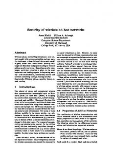
4 Simulation Results The transmission power, the signal attenuation, and the reception sensibility are taken into account to evaluate the transmission and the interference ranges for the different data rates of the 802.11 ad hoc network. We assumed a transmission power of 18 dBm, or 63.1 mW [8]. The path-loss model is used to compute the channel attenuation and, consequently, the transmission range of all the scenarios. We consider the propagation loss parameter β = 3.9 [9] for all urban scenarios and β = 3.0 for the rural scenario due to its lower density of residences. Thus, the interference range is equal to 74 m for Scenarios 1 to 4 and equal to 269 m for Scenario 5, which is also calculated with the path-loss model. The Internet gateway is always positioned at the center of each scenario or at one of its vertices. The results obtained have a confidence interval of 95%. 4.1 Connectivity Analysis The connectivity analysis is of utmost importance because the collaborative communications provided by an ad hoc network must consider that the terminals may not be turned on all the time. The different scenarios use real values for residential area and density. Therefore, there may be from 7,000 to 61,000 terminals. Hence, a specific simulator written in C was implemented to analyze the connectivity. The simulator implements the Dijkstra algorithm to calculate the shortest path to the gateway and computes the percentile of connected nodes as well as the average number of hops to the gateway. A terminal is connected when it has at least one path to the gateway. We use physical transmission rates from 1 to 54 Mbps. The connectivity is evaluated as a function of the percentage of nodes on that are randomly chosen for each simulation run. In Figures 1(a) and 1(b),
Wireless Ad Hoc Networks on Underserved Communities 100
80
1Mbps
60
54Mbps 11Mbps
40 20
36Mbps
Terminals connected (%)
Terminals connected (%)
100
0
80
1Mbps
60
54Mbps
11Mbps 36Mbps
40 20 0
0
20
40 60 Terminals on (%)
80
100
(a) Connectivity - GW at the vertex. 140
0
140
36Mbps
80
11Mbps
60 1Mbps 40 20
40 60 Terminals on (%)
80
100
54Mbps
120 Number of hops
100
20
(b) Connectivity - GW at the center.
54Mbps
120 Number of hops
191
100
36Mbps
80 11Mbps 60 40
1Mbps
20
0
0 0
20
40 60 Terminals on (%)
80
(c) Hops - GW at the vertex.
100
0
20
40 60 Terminals on (%)
80
100
(d) Hops - GW at the center.
Fig. 1. Scenario 1 - Rocinha.
high network connectivity is achieved in Scenario 1 at the four simulated transmission rates. Nevertheless, when the gateway is positioned at the center of the scenario, high connectivity can be reached with a smaller percentage of nodes on. At 11 Mbps, when the gateway is in the center of the scenario, only 20% of the nodes need to be on to achieve high connectivity. With the gateway at one vertice, high connectivity only happens when 30% of the nodes are on. Figures 1(c) and 1(d) show that the average number of hops increases with the number of nodes on. In the beginning, only a few nodes are connected. Thus, there is a higher probability for the nodes near the gateway to be connected than for the nodes further from the gateway. As the further nodes get connected, the average number of hops increases. This is true until the network gets fully connected. After that, the average number of hops decreases because, as new nodes get into the network, new and smaller routes to the gateway are found. The results of Scenarios 2 and 4 are similar to Scenario 1, therefore they were omitted. In Scenario 3, Figures 2(a) and 2(b) show that, independently of the percentage of terminals on, the network connectivity is near zero for 36 and 54 Mbps. This is due to a smaller number of neighbors. Despite being the more populated scenario, the average density for each XY plane is smaller than in Scenarios 1 and 2. The average density is 2500 residences/floor, assuming a 10-floor building. This density is almost five times smaller than in Scenario 1.
192
Campista et al. 100
80
Terminals connected (%)
Terminals connected (%)
100 1Mbps 36Mbps−6dBi 11Mbps 54Mbps−6dBi
60 40
54Mbps 36Mbps
20
80
1Mbps 36Mbps−6dBi 11Mbps 54Mbps−6dBi
60 40
54Mbps 36Mbps
20
0
0 0
20
40 60 Terminals on (%)
80
100
(a) Connectivity - GW at the vertex.
0
20
12 Number of hops
Number of hops
11Mbps 36Mbps−6dBi 6 1Mbps 4 54Mbps
2 0
20
40 60 Terminals on (%)
10 8 6
54Mbps
4 2
36Mbps
0
100
54Mbps−6dBi 11Mbps 36Mbps−6dBi 1Mbps
54Mbps−6dBi 8
80
(b) Connectivity - GW at the center.
12 10
40 60 Terminals on (%)
80
(c) Hops - GW at the vertex.
36Mbps
0 100
0
20
40 60 Teminals on (%)
80
100
(d) Hops - GW at the center.
Fig. 2. Scenario 3 - Copacabana.
Nevertheless, antennas can be used to assure high connectivity at higher transmission rates in Scenario 3. Figures 2(a) and 2(b) plot the results obtained with 6 dBi antennas. The average number of hops for Scenario 3 is depicted in Figures 2(c) and 2(d). It is observed that the variation of the average number of hops is small increasing the percentage of nodes on and the transmission rates. Since high network connectivity can be achieved with a small number of nodes on, adding more to the network does not affect the average number of hops. Besides, the average number of hops in Scenario 3 is smaller than seen in Scenario 1. As high connectivity is reached at smaller rates, the transmission range is higher and the average number of hops to the gateway gets lower. In Scenario 5, Figures 3(a) and 3(b) show that it is impossible to achieve high network connectivity with the specified values of the IEEE 802.11 standard without antenna. Only at 1 Mbps we can reach connectivity. Using the gateway at the center or at the vertex of the scenario, the deployment of an antenna with a gain of 6 dBi provides connectivity for more than 95% of the nodes with at least 60% of the nodes on. As in Scenario 3, the average number of hops is also smaller than in Scenario 1. This is due to the great distances between neighbor nodes, which is a characteristic of rural regions. The results show the benefits of the gateway located at the center of the simulated area. Independent of the scenario, for distinct transmission rates,
Wireless Ad Hoc Networks on Underserved Communities 100 1Mbps−12dBi
80
1Mbps−6dBi 11Mbps−12dBi
60 40
11Mbps−6dBi 1Mbps
20
24Mbps−12dBi
Terminals connected (%)
Terminals connected (%)
100
1Mbps−12dBi
80
1Mbps−6dBi 11Mbps−12dBi
60 40
11Mbps−6dBi 1Mbps
20
24Mbps−12dBi
0
0 0
20
40
60
80
100
0
20
40
Terminals on (%)
60
80
100
Terminals on (%)
(a) Connectivity - GW at the vertex.
(b) Connectivity - GW at the center.
45
45
40
24Mbps−12dBi
40
35 30 11Mbps−12dBi 25
1Mbps−6dBi
20
1Mbps−12dBi
11Mbps−6dBi
15 10
Number of hops
Number of hops (%)
193
24Mbps−12dBi
35
11Mbps−6dBi
30
1Mbps
25
1Mbps−6dBi
20
11Mbps−12dBi
15 10
1Mbps
5
1Mbps−12dBi
5
0
0 0
20
40 60 Terminals on (%)
80
(c) Hops - GW at the vertex.
100
0
20
40 60 Terminals on (%)
80
100
(d) Hops - GW at the center.
Fig. 3. Scenario 5 - Paty do Alferes.
high connectivity can be achieved with a small percent of nodes on. Besides, the average number of hops is smaller when the gateway is at the center. 4.2 Capacity Analysis The capacity analysis evaluates the impact of the number of hops over the throughput of a one-node transmission and the network aggregated throughput when increasing the number of transmitting terminals. We developed an IEEE 802.11g module for ns-2 version 2.28 [10]. We used a lower number of terminals due to the limitations of ns-2, but we kept the density of nodes used in Section 3. The transmission rates used in each scenario are chosen depending on the results of the connectivity analysis, Section 4.1. We use the highest transmission rate that offers 100% of connectivity when all nodes are on. The gateway is located in one of the vertices. The terminals send 1500 data packets using CBR/UDP, there is neither packet segmentation nor deployment of RTS/CTS mechanism. Where IEEE 802.11g can be deployed, the use of short slot time is assumed. Forwarding Chain In this simulation set the impact of the number of hops over the throughput is shown. The number of terminals in the network and the data rates are varied. The data rate is varied from 56 kbps to 54 Mbps.
194
Campista et al.
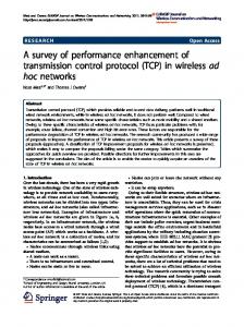
In Scenario 1, the number of terminals is varied from 4 to 196. The gateway is positioned at one vertex of the grid and the transmitting terminal is located at the opposite vertex of the diagonal. The distance among terminals is 9.09 m and the transmission rate is 54 Mbps. At this rate, the transmission range is approximately 12.6 m. The interference range is 74 m. The maximum throughput of IEEE 802.11g is about 29 Mbps for an onenode transmission [10]. In Scenario 1, for 4 terminals, the route has two hops because the diagonal path cannot be reached due to transmission range constraints. Nevertheless, as the interference range is higher than the transmission range, simultaneous transmissions are not possible. Thus, the source and the intermediate terminals share the maximum throughput approximately by two as seen in Figure 4(a). While the added terminals are inside the source interference range, the maximum throughput is divided by the number of intermediate terminals that compose the forwarding chain [6]. Adding terminals outside the interference range of the source allows simultaneous transmissions. Therefore, increasing the network with terminals further from the source allows spatial reuse in the forwarding chain. In Figure 4(a), it is observed that when the spatial reuse starts, the throughput of the forwarding chain tends to be constant. Figure 4(a) shows that for data rates of 56 kbps, 512 kbps, and 1 Mbps, the network is not saturated. On the other hand, the maximum throughput of the forwarding chain is constant and near 2 Mbps. Increasing the distance between the source and the gateway, the user may still get a reasonable throughput. The results obtained for Scenarios 2 and 4 are similar to the results of Scenario 1. Therefore, they were omitted. Scenario 3 simulates a region composed by buildings. Thus, in this scenario, the nodes are in a three-dimensional grid as detailed in Section 3. The gateway and the source terminal are located at the opposite vertices of the diagonal of the cube. To keep density, the nodes are 20 m away in the XY plane. The maximum possible data rate is 11 Mbps to maintain connectivity, as depicted in Figure 2. At this rate, the transmission range is 32 m. As mentioned before, the interference range is 74 m. The maximum throughput obtained with only one source-destination pair is about 7 Mbps. This is the 10-node throughput seen in Figure 4(b). With 10 nodes, there is a one-hop transmission because the source-destination pair is 30 m away in the same building. This justifies the maximum throughput of 7 Mbps since there is only one node contending for the medium. From 40 nodes on, more hops are necessary and, consequently, the throughput decreases. As in Scenario 1, the throughput goes down while the added nodes are inside the interference range of the source. When the added nodes are located out of the interference range of the source, the throughput tends to a constant due to spatial reuse. In Scenario 3, this throughput is about 1.2 Mbps. It is worth noting that in Scenarios 1 the throughput of the forwarding chain gets constant about 2 Mbps considering a physical transmission rate of 54 Mbps. In Scenario 3, at 11 Mbps, the constant throughput is about 1.2 Mbps. This is due to a higher efficiency of IEEE 802.11b compared to 802.11g. Although
Wireless Ad Hoc Networks on Underserved Communities 16
7 54Mbps
12
11Mbps
10
6 1Mbps 512kbps
8
56kbps
6 4
Throughput (Mbps)
Throughput (Mbps)
14
54Mbps
5
1Mbps
4
11Mbps
512kbps
3
56kbps
2 1
2 0
0 0
20 40 60 80 100 120 140 160 180 200
0
50
Number of terminals
0.12 0.1 0.08 0.06 0.04
0.4
300
350
400
11Mbps 1Mbps
0.3
512kbps
0.25 0.2 0.15 0.1 0.05
(c) Scenario 5 - Paty do Alferes.
250
54Mbps
0.35
0 10 20 30 40 50 60 70 80 90 100 Number of terminals
200
(b) Scenario 3 - Copacabana.
0.02 0
150
0.45 Throughput (Mbps)
56kbps 512kbps 1Mbps 11Mbps 54Mbps
0.14
100
Number of terminals
(a) Scenario 1 - Rocinha. 0.16 Throughput (Mbps)
195
56kbps 0
10 20 30 40 50 60 70 80 90 100 Number of terminals
(d) Scenario 5 - With connectivity.
Fig. 4. Forwarding chain throughput.
the data rates of 802.11g can reach up to 5 times the data rates of 802.11b, the control frames are transmitted in lower rates to maintain interoperability. This affects the 802.11g efficiency [10]. Scenario 5 is a rural environment. In this scenario, the nodes are randomly located and the distances, in average, are larger than in the other scenarios. According to Figure 3, it is necessary to use low transmission rates and antennas to achieve connectivity. Therefore, we use a transmission rate of 1 Mbps and antenna gain of 12 dBi. The gateway and the source are at the opposite vertices of the simulation square. Figures 4(c) and 4(d) show the results obtained. In Figure 4(c), the error bars are big and thus the results are not conclusive. This is due to lack of connectivity between gateway and source terminal in some simulation runs. As the intermediate nodes are randomly located, non-connectivity events may happen forcing the throughput down to zero. The average throughput of the runs with and without connectivity results in points with a high variance. Eliminating the non-connectivity points (Figure 4(d)) we can observe a tendency of the throughput which is similar to the other scenarios. For a large number of nodes a throughput near to 150 kbps is achieved. Thus, the use of IEEE 802.11 is possible in rural environments but depends on antennas and the access terminals location.
196
Campista et al.
IEEE 802.11 wireless ad hoc networks are suitable for urban scenarios, but not as suitable to rural environments. Besides, considering one-node transmissions, the throughput obtained can be up to 2 Mbps regardless the distance between gateway and source terminal. This throughput value must be lower if more than one node contends for the medium. The following simulation set focuses on the saturation throughput for multiple sources. Network Throughput This simulation set verifies the maximum number of users before saturation and the performance of two routing protocols, the reactive AODV and the proactive OLSR. The AODV module is already available in the ns-2 distribution. On the other hand, to simulate OLSR it is necessary to add a patch to the simulator [11]. The nodes always send data at 56 kbps and the transmission rate of each scenario is the same used in Section 4.2. The transmission rate of Scenario 1 is 54 Mbps. Figure 5(a) shows that independently of the routing protocols, the saturation is achieved for approximately 60 nodes. It is observed in both curves that after saturation, the throughput decreases until it gets stable. This behavior is typical of CSMA protocols without collision detection. In Figure 5(a) it is also observed that when every node is transmitting, unlike Figure 4(a), the maximum throughput is higher than 3 Mbps. This occurs due to spatial reuse, which allows simultaneous transmissions. The effect of spatial reuse starts after 36 nodes, when the diagonal of the grid is larger than the interference range of the source. The difference in throughput between AODV and OLSR is due to the higher control overhead of OLSR. The OLSR protocol is proactive, flooding the network periodically to keep the routing tables updated. The results of Scenarios 2 and 4 were omitted because they are similar to Scenario 1. In Scenario 3, IEEE 802.11b is used at 11 Mbps as in the forwarding chain analysis. Figure 5(b) shows that after saturation the aggregated throughput goes down and for a higher number of nodes it is supposed to become stable as in Figure 5(a). The performance of OLSR overcomes AODV because OLSR deploys special nodes called MPR (MultiPoint Relay). The MPR is a node chosen to send control packets. Each node chooses an MPR set per interface. This set comprises the minimum number of one-hop neighbors that can reach every two-hop neighbor. Thus, only the MPRs transmit packets to two-hop neighbors, limiting the flooding. In Scenario 3, the deployment of MPRs is more efficient than in Scenario 1 due to the number of nodes inside the same transmission range. In Scenario 1, the distance among nodes is 9.09 m and the transmission range is 12.6 m. Therefore, every node have only four neighbors and the MPRs produce no gains because all nodes are all MPRs. In Scenario 3, instead, the transmission range is 32 m and the distance among the nodes in the XY plane is 20 m. In this case, the number of neighbors is eight, plus the neighbors in the Z axis. Increasing the number of neighbors improves the performance of the MPRs because the flooding decreases. In Scenario 5, the random position of the nodes and the low density affect the results. Using IEEE 802.11 at 1 Mbps and antennas as in Figure 3, it is not
Wireless Ad Hoc Networks on Underserved Communities 4
3.5
3.5
3 Throughput (Mbps)
Throughput (Mbps)
197
3 2.5 2 1.5
AODV
1
OLSR
2.5 2 1.5
0.5
0.5
0
0 20
40
60
80
100
120
140
OLSR
1
AODV 20
40
Number of terminals
60
80
100
120
140
160
Number of terminals
(a) Scenario 1 - Rocinha.
(b) Scenario 3 - Copacabana.
0.26 Throughput (Mbps)
0.24 0.22 0.2 0.18 0.16 0.14 0.12 0.1 0.08
AODV−6dBi OLSR−6dBi AODV−12dBi OLSR−12dBi 10 20 30 40 50 60 70 80 90 100 Number of terminals
(c) Scenario 5 - Paty do Alferes. Fig. 5. Network aggregated throughput.
possible to assure that the gateway is connected to the rest of the network in every simulation run. For the same reasons pointed out in the forwarding chain analysis, the variance is high as seen in Figure 5(c). AODV tends to present a better throughput than OLSR. Again, the low density hinders the MPRs gains. Also, note that even increasing with number of nodes, the saturation is not achieved. This happens because the number of nodes that transmit is limited to the nodes closer to the gateway.
5 Conclusions The return channel of the digital TV can be used as a low-cost vehicle for digital inclusion of underserved communities. A viability analysis of the return channel must be considered to certify that the ad hoc technology is suitable. In the connectivity analysis, we verified that in urban regions it is possible to achieve high connectivity with a reduced number of terminals turned on. Besides, in highly populated regions, 802.11 transmission rates up to 54 Mbps can be used. On the other hand, in rural regions, the deployment of antennas and the use of low transmission rates are mandatory to increase the transmission range and guarantee connectivity. Positioning the gateway at the center of the scenarios, 100% of connectivity is possible with a fewer number of nodes on
198
Campista et al.
compared to the vertex-positioned gateway. The average number of hops is also lower when the gateway is at the center. In the capacity analysis, we considered different numbers of nodes keeping the density of residences constant. The results obtained by the forwarding chain showed that increasing the distance between the gateway and the source terminal, the user could obtain a reasonable throughput with an ad hoc return channel. For a large number of nodes, the throughput of the forwarding chain approximates to a constant which can be up to 2 Mbps. We also verified that the saturation occurs around 60 access terminals sending data at 56 kbps regardless of the routing protocol. This data rate corresponds to a dial-up connection and fits well the of the digital TV applications. For dense scenarios, the OLSR routing protocol shows a better throughput than AODV. On the other hand, in sparse scenarios, the AODV routing protocol is more suitable than OLSR. As a consequence, currently, we investigate the implementation of a routing protocol specific to the ad hoc return channel.
References 1. IBGE, “PNAD 2003 - National Research using Residences Sampling (In Portuguese),” 2004, http://www.ibge.gov.br/home/estatistica/populacao/ trabalhoerendimento/pnad2003/sintesepnad2003.pdf. 2. J. Hsu, S. Bhatia, K. Tang, R. Bagrodia, and M. J. Acriche, “Performance of Mobile Ad Hoc Networking Routing Protocols in Large Scale Scenarios,” in MILCOM’04, Oct. 2004, pp. 21–27. 3. J. Hsu, S. Bhatia, M. Takai, R. Bagrodia, and M. J. Acriche, “Performance of Mobile Ad Hoc Networking Routing Protocols in Realistic Scenarios,” in MILCOM’03, Oct. 2003, pp. 1268–1273. 4. S. Armenia, L. Galluccio, A. Leonardi, and S. Palazzo, “Transmission of VoIP Traffic in Multihop Ad Hoc IEEE 802.11b Networks: Experimental Results,” in WICOM’05, July 2005, pp. 148–155. 5. E. Borgia, “Experimental Evaluation of Ad Hoc Routing Protocols,” in PERCOMW’05, Mar. 2005, pp. 232–236. 6. B. A. M. Villela and O. C. M. B. Duarte, “Maximum Throughput Analysis in Ad Hoc Networks,” in Networking’04, May 2004, pp. 223–234. 7. IBGE, “Cidades@,” 2005, http://www.ibge.gov.br/cidadesat/. 8. H. Bengtsson, E. Uhlemann, and P. Wiberg, “Protocol for wireless real-time systems,” in 11th Euromicro Conference on Real-Time Systems, June 1999. 9. S. Zvanovec, P. Pechac, and M. Klepal, “Wireless LAN Networks Design: Site Survey or Propagation Modeling?” RADIOENGINEERING, vol. 12, no. 4, pp. 42–49, Dec. 2003. 10. A. Amodei Jr., M. E. M. Campista, D. de O. Cunha, P. B. Velloso, L. H. M. K. Costa, M. G. Rubinstein, and O. C. M. B. Duarte, “Analysis of medium access control protocols for home networks,” UFRJ - Brazil, Tech. Rep., Oct. 2005. 11. Francisco J. Ros, “OLSR-UM Documentation,” Mar. 2005, http://masimum.dif.um.es/um-olsr/html/.