wireless capsule endoscopy image classification based on vector ...

WIRELESS CAPSULE ENDOSCOPY IMAGE CLASSIFICATION BASED ON VECTOR SPARSE CODING Tao Ma1, Yuexian Zou1*, Zhiqiang Xiang1, Lei Li1 and Yi Li2 1 ADSPLAB/ELIP, School of ECE, Peking University, Shenzhen 518055, China 2 Shenzhen JiFu Technology Ltd. {*[email protected]} ABSTRACT 1

Wireless capsule endoscopy (WCE) is a promising technology for gastrointestinal disease detection. Since there are more than 50,000 frames in one WCE video of a patient, classifying the whole frame set of the digestive tract into subsets corresponding to esophagus, stomach, small intestine, and colon is necessary, which can help physicians review and diagnose rapidly and accurately. The digestive organ classification in WCE is a challenging task due to the difficulties in feature representation of WCE images. This paper presents a new method of WCE organ classification by incorporating a proposed locality constraint based vector sparse coding (LCVSC) algorithm with the support vector machine classifier. Experimental results validate the effectiveness of the proposed method and it is encouraging to see that a good classification performance is achieved.

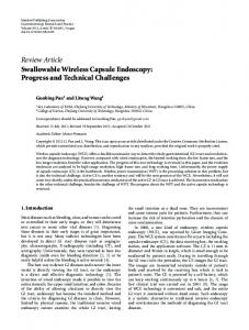
(a) (b) (c) (d) Fig. 1. Image samples of the digestive organs: (a) esophagus; (b) stomach; (c) small intestine; (d) colon.

50,000 frames and it will take about two or more hours for an experienced physician to assess one WCE video, which is too time-consuming and limits the number of examinations. For promoting the practical applications of the WCE technique, the automatic classification of the digestive organs is required, which will let the physicians locate the organs easily and help the physicians to reduce the assessment time. Typical samples of the digestive organs are shown in Fig. 1. Generally computer vision based methods can be employed to discriminate the digestive organs including esophagus, stomach, small intestine, and colon. Vision-based automatic classification of digestive organs is a typical pattern recognition problem. Most previous works follow the general framework including image feature representation and classifier design. There are some solutions proposed for solving the problem. Berens et al. [3] proposed a method of automatically discriminating stomach, intestine and colon tissue by computing hue saturation chromaticity histograms which are compressed using a hybrid transform, incorporating the DCT and PCA. The Knearest neighbor (KNN) classifier and the Support Vector Machine (SVM) were adopted and the performance comparisons were given. Cunha et al. [4] extracted MPEG-7 descriptors as low-level image features, and then the SVM classifier and Bayesian classifier have been employed. The research showed that using SVM instead of Bayesian significantly improves the classification results. In [5], a feature vector combining color, texture, and motion information was created and the images extracted from the WCE video were classified into meaningful parts (esophagus, stomach, small intestine, and colon) using the nonlinear SVM built within the framework of a hidden Markov model. In this paper, aiming to develop an effective WCE organ classification method, we first use the SIFT (scale invariant

Index Terms— wireless capsule endoscopy, digestive organs, image classification, vector sparse coding 1. INTRODUCTION Wireless Capsule Endoscopy (WCE) is a novel technology for recording the videos of the digestive tract of patients, which was first appeared in [1] and put in use by Given Imaging Ltd., Israel in 2001. WCE uses a small 11×26-mm capsule, one end of which contains an optical dome with white light emitting diodes (LEDs) and a color camera that captures about two images per second. When a WCE is swallowed by a patient, it will be propelled by peristalsis to move through the gastrointestinal tract, and the captured images are transmitted to a data recorder by using the wireless communication channel. Compared with traditional endoscopy, the main advantages of WCE are that patients can avoid cross infection and suffer no pain. WCE also brings great benefits to elder and weak patients [2]. However, the WCE video of one patient contains more than 1

This work was supported by the Shenzhen Science & Technology Fundamental Research Program (No: JCYJ20130329175141512) and the collaboration research project funded by Shenzhen JiFu Technology Ltd. The authors would thank Shenzhen JiFu Technology Ltd. for providing the WCE image dataset.

978-1-4799-5403-2/14/$31.00 ©2014 IEEE

582

ChinaSIP 2014

feature transform) descriptors [7] to capture the discriminative information and give a robust primary representation of WCE images. Then the proposed locality constraint based vector sparse coding (LCVSC) algorithm is used to map all the extracted SIFT vectors into a sparse feature domain, where the linear SVM classifier can be adopted to achieve encouraging classification performance. Since the linear SVM asks for much lower computational complexity in training and testing compared with the nonlinear SVM [6], it is preferred over the nonlinear SVM to provide the tradeoff between computational complexity and classification accuracy in practical applications of the WCE technique, where the scalability of training and the speed of testing are very important. The system framework of our proposed method is shown in Fig. 2. In the rest of this paper, Section 2 describes the feature representation of WCE images, including the SIFT extraction and vector sparse coding on SIFT feature vectors. Section 3 introduces the supervised classification using the linear SVM classifier. Section 4 shows the experimental results and Section 5 gives the conclusion.

Input WCE Images

Feature Representation

Spatial Pooling

Linear SVM (Decision)

Organ Types

Linear SVM (Training)

Fig. 2. The system framework of the proposed method for WCE digestive organ classification.

image Is, each 128×1 SIFT-FV is extracted from a 16×16 pixel patch, and the SIFT-FVs are densely sampled on the regular grid with the stepsize of 8 pixels. All the extracted SIFT-FVs constitute the SIFT feature matrix Ys. 2.2. Vector Sparse Coding on SIFT Descriptors In general, sparse coding consists of two phases: dictionary learning and vector sparse coding. Let  = [y1, … , yN] be a matrix formed by a set of SIFT-FVs, where yi (i = 1, 2, … , N) is a M×1 (M = 128) SIFT-FV and N is the total number of the SIFT-FVs in . The sparse coding method proposed by Yang et al. in [11] is based on the following optimization:

2. FEATURE REPRESENTATION

N min   yi  Dxi X ,D  i 1

We consider use the grayscale images in the WCE organ classification. Each WCE image is firstly converted into a grayscale image as the input of feature representation. To facilitate the description, let Is denote a WCE image. Ys is the SIFT feature matrix of Is, which consists of all the SIFT feature vectors extracted from Is. Xs denotes the sparse matrix obtained by doing the vector sparse coding on each SIFT feature vector in Ys.

s.t.

dj

2

2 2

   xi 1  

(1)

 1, j  1, 2,..., L

where D = [d1, … , dL] is the M × L dictionary and dj (j = 1, 2, … , L) denotes an M × 1 base vector in D. L is generally greater than M to obtain an over-complete dictionary. X = [x1, … , xN] denotes the sparse matrix formed by the sparse vectors associated with , and xi (i = 1, 2, … , N) is the L × 1 sparse coded vector obtained by coding yi over D. The L1norm (||.||1) of xi is the sparsity regularization term and  is a free parameter that enforces the sparsity of the solution. Lee et al. [12] proved that (1) is an optimization problem which is not convex in both X and D simultaneously, but it is convex in X when D is fixed and convex in D when X is fixed. The conventional procedure for the optimization in (1) is to solve it iteratively by alternatingly optimizing over D or X while fixing the other. When D is fixed, Eq. (1) can be processed by optimizing over each xi individually as follows:

2.1. SIFT Extraction SIFT descriptor is empirically shown to outperform many other local features [8] for image classification. A SIFT feature vector (SIFT-FV) is created by first computing the gradient orientation and magnitude at each image sample point in a region around an anchor point. The region is partitioned into r×r subregions. A gradient orientation histogram for each subregion is then formed by accumulating samples within the subregion, weighted by the corresponding gradient magnitudes. All orientation histograms from subregions are concatenated to give a SIFT-FV [9, 10]. Generally, the SIFT-FV with the best performance is extracted from every 16×16 pixel patch, which is divided into 4×4 subregions. Then, the obtained 4×4 array of histograms with 8 orientation bins in each creates one 128-by-1 SIFT-FV (4×4×8). Motivated by the effective image representation ability of densely sampled SIFT descriptors [7], we use a dense regular grid instead of commonly adopted interest points to extract SIFT feature vectors, which turns out to capture more discriminative information of WCE images. For



min yi  Dxi xi

2 2

  xi

1



(2)

This is essentially a linear regression problem with L1-norm regularization on xi. Eq. (2) can be solved efficiently by using the feature-sign search algorithm [12]. When X is fixed, the optimization in (1) can be reduced to the following: min   DX D

2 F

s.t. d j

2

 1, j  1, 2,..., L

(3)

Eq. (3) is a least square problem with L2-norm constraints on each base vector dj in D. The Lagrange dual algorithm

583

proposed in [12] can be employed to efficiently solve (3). As mentioned before, sparse coding has a dictionary learning phase and a vector sparse coding phase. The algorithm to obtain the dictionary D is summarized in Table I, where the input SIFT matrix  needs to be given. In our implementation, we collected 5,000 WCE images including various esophagus, stomach, small intestine, and colon images to extract SIFT-FVs from patches. As a result, about 1,000,000 SIFT-FVs are obtained and used to form the  for dictionary learning. In the vector sparse coding phase, Eq. (1) is solved with respect to X only when D is available and fixed. The sparse coded vector xi of each SIFT-FV yi will be obtained by solving the L1-norm optimization in (2).

Table I. The dictionary learning algorithm.

Input: The given SIFT matrix  = [y1, … , yN]. Initialization: Randomly generate L base vectors in D, each of which is normalized to a unit vector. Repeat 1: Fixing D, Eq. (2) is solved for each yi to form a temporary X. 2: Fixing X, Eq. (3) is solved to get a temporary D. Until the maximum number of iterations is exceeded. Output: The final D is the dictionary we want. The WCE organ classification is implemented by a SVM classifier. Firstly, we need to prepare the training and testing samples of SVM. Each sample, which is a feature vector denoted by zs, represents the final feature representation of image Is. The spatial pyramid matching (SPM) proposed in [7] is adopted in the spatial pooling phase to get the final feature vector for each image. The SPM method partitions an image into 2b ×2b segments in different scales b = 0, 1, 2. For each of the 21 subregions, the sparse coded vectors within it are pooled together with a pooling function to get the corresponding pooled sparse coded vector (PSCV). For ease of explanation, let zs(p,q,b) denote the resulting PSCV of the (p,q)-th subregion in the b-th scale of Is. Careful evaluation shows that the max pooling function outperforms other alternative pooling functions, such as the mean of absolute values and the mean square root. Hence, the spatial pooling in each subregion is based on the following equation: (6) zsj ( p, q, b)  max{x j1 , x j 2 ,..., x jT }, j  1, 2,..., L

2.3. Locality Constraint Based Vector Sparse Coding To favor sparsity, common sparse coding algorithm might select quite different bases from the dictionary for coding similar SIFT-FVs, which means that similar image patches might have quite different sparse codes. To achieve good classification performance, the coding scheme should generate similar sparse codes for similar SIFT descriptors, which asks for capturing the correlations between similar descriptors by sharing the bases in D. In this subsection, we propose the locality constraint based vector sparse coding (LCVSC) algorithm to improve the traditional sparse coding algorithm described in Section 2.2 by introducing the locality constraint. When the dictionary D is obtained as detailed in Section 2.2 and Table I , instead of coding each yi by solving Eq. (2) directly, we first perform a K-nearest-neighbor (KNN) search in D to build the local base set Di for each input SIFT-FV yi. In our study, the dj and yi are normalized. The similarity between dj and yi in KNN is measured as:

where zsj ( p, q, b) is the j-th element of the PSCV zs(p,q,b), xjt denotes the j-th element of the t-th sparse coded vector in the (p,q,b)-th subregion, and T is the total number of sparse coded vectors within the subregion. L is the dimension value of each sparse coded vector which is equal to the number of bases in D. When the max pooling across all the subregions of a WCE image is finished, all these PSCVs from 21 subregions are then directly concatenated and normalized to form the final feature vector zs of the image Is. A multiclass linear SVM classifier is employed to classify the WCE images into different digestive organs. We take the widely used one-vs-all (OVA, or one-vs-rest) strategy to train m binary linear SVM classifiers for building the multiclass linear SVM classifier, where m is the number of classes that need to be classified.

M

Sim( yi , d j )   yik  d jk

(4)

k 1

where yik and djk represent the k-th element of yi and dj, respectively. After KNN searching we can obtain the local base set Di which consists of K base vectors that are most similar to yi. Then yi can be encoded over Di instead of over D via the following minimization problem:



min yi  Di xi xi

2 2

  xi

1



(5)

where xi is the K-by-1 sparse coded vector associated with Di. To keep the good discriminative ability of highdimensional feature representation, xi is then projected to the L-dimensional sparse feature domain to generate the Lby-1 sparse coded vector xi, and the coefficients in xi corresponding to the (L−K) unselected bases in D are set to 0. Moreover, as K is usually smaller compared with L, solving (5) is faster than directly solving (2) due to the smaller size of dictionary.

4. EXPERIMENTAL RESULTS 4.1. Experimental Setup As WCE is a medical frontier technology, there is no public WCE dataset for performance assessment. The dataset we used is provided by Shenzhen JiFu Technology Ltd., which was captured from 5 trial patients. The size of each image is of 480×480 pixels. Four digestive organs are considered to

3. SUPERVISED WCE ORGAN CLASSIFICATION

584

be classified: esophagus, stomach, small intestine, and colon. We collected 9,000 WCE images by random selection from the whole dataset, including 1,000 esophagus images, 2,000 stomach images, 3,000 small intestine images, and 3000 colon images. Each image has been labeled by the provider with the corresponding organ class for evaluating the performance. To compare with our proposed locality constraint based vector sparse coding (LCVSC) method, we also implemented two very popular image classification methods. One is the method that using traditional cluster-based vector quantization (K-means) to coding the input descriptors, which is proposed in [7] and termed as the CVQC method in this section. The other is the common L1-norm constraint based vector sparse coding method proposed in [11] as described in Section 2.2, which is termed as L1-norm-VSC here. For performance comparison purpose, three methods follow the same framework of SIFT-Coding-SPM-SVM but with different coding algorithms. Simulation parameters are set as follows. Each WCE image is resized to 120×120 pixels using the bicubic interpolation to reduce the computational cost. For CVQC [7], the codebook size is fixed as 512 which achieves optimal performance. For L1-norm-VSC [11] and our proposed LCVSC, the dictionary size L is selected to be 1024 as used in [11], and the free parameter used in Eq. (2) and Eq. (5) is set as 0.15 empirically. For our proposed LCVSC, K is set to 256. 4.2. Experimental Results Following the common benchmarking procedure of multiclass classification, we repeat the classification by 10 times with different random selection of the SVM training and testing images. The training set was formed by using 50, 100, 200, and 400 images per digestive organ class respectively. The testing set is formed by the rest. For each trial, per-class accuracy values are recorded and their average value is computed. Then we report the final averaged classification accuracy by the mean of the results from the individual trials. The experimental results are shown in Table II. From the results, we can see that the increase of the SVM training size leads to better classification accuracy for all the three methods. For all the cases of training size, the proposed LCVSC method outperforms CVQC by 4 ~ 6 percent, and outperforms L1-norm-VSC by more than 1 percent. To evaluate the impact of the parameter K on the classification performance of the proposed LCVSC, one experiment is conducted. Five different values of K have been tested: 64, 128, 256, 512, and 1024, and 400 training images per organ class are used. The results are given in Table III. It is clear to see that the classification accuracy varies with different K values, and smaller K and bigger K give inferior performance. The best selection of K is 256 under this experimental setup. Intuitively, if K is too small,

585

Table II. Averaged classification accuracy comparison. SVM training images (per class) CVQC [7] L1-norm-VSC [11] LCVSC (proposed)

50

100

200

88.75% 94.28% 95.54%

91.93% 95.46% 96.62%

92.83% 96.25% 97.49%

400 94.67% 97.78% 98.79%

Table III. The effects of the number of nearest-neighbors on the proposed method. K Accuracy

64 92.54%

128 97.92%

256 98.79%

512 98.13%

1024 97.76%

Table IV. The confusion matrix for CVQC/L1-norm-VSC/LCVSC. Predicted Class → Esophagus Stomach Small Intestine Colon

Small Intestine 575/583/594 18/11/4 3/2/0 32/14/6 1490/1538/1561 56/ 32/24 Esophagus

Stomach

11/4/0

23/10/7

53/10/12

39/9/6

Colon 4/4/2 22/16/9

2545/2582/2590 107/24/15

21/4/3

2401/2557/2567

the local base set Di loses the ability to represent the input features which leads to lower discriminant power; if K is too large, the locality constraint gets weaker and the LCVSC will be close to L1-norm-VSC. To further demonstrate the classification ability of the algorithms, a confusion matrix between the four digestive organs averaged over 10 trials for the three methods is computed and shown in Table IV. In this experiment, 400 training images per class and K=256 are used. It is noted that there are 600 esophagus images, 1,600 stomach images, 2,600 small intestine images, and 2,600 colon images in the testing set. In Table IV, each element records the number of correct classification or misclassification by using the CVQC, L1-norm-VSC, and LCVSC respectively. From the confusion matrix, we can see that the proposed LCVSC outperforms CVQC and L1-norm-VSC in almost every organ class. It is noted that the highest number of misclassification occurs between the adjacent organs, such as stomach / small intestine and small intestine / colon, for all the methods. The proposed LCVSC obtained the lowest misclassification as well. 5. CONCLUSION A new method has been proposed to achieve good digestive organ classification accuracy for the large volume of the WCE images under the SIFT-Coding-SPM-SVM framework, where the locality constraint based vector sparse coding (LCVSC) method has been developed to obtain better discriminative feature representation capacity. Intensive experiments have been carried out to evaluate the classification performance. It is encouraging to see that the proposed WCE digestive organ classification system is able to achieve the averaged classification accuracy higher than 95% for almost all testing trials. Future work will focus on further reducing the computational cost.

REFERENCES [1] G. Iddan, G. Meron, A. Glukhovsky, et al., “Wireless capsule endoscopy,” Nature, Vol. 405, pp. 725-729, 2000. [2] L. Li, Y. X. Zou, and Y. Li, “Wireless capsule endoscopy images enhancement based on adaptive anisotropic diffusion,” in IEEE China Summit & International Conference on Signal and Information Processing (ChinaSIP), pp. 273-277, 2013. [3] J. Berens, M. Mackiewicz, and D. Bell, “Stomach, intestine, and colon tissue discriminators for wireless capsule endoscopy images,” in Proc. of SPIE Conference on Medical Imaging, Vol. 5747, pp. 283-290, Bellingham, WA, April 2005. [4] J. P. S. Cunha, M. Coimbra, P. Campos, et al., “Automated topographic segmentation and transit time estimation in endoscopic capsule exams,” IEEE Transactions on Medical Imaging, Vol. 27, pp. 19-27, 2008. [5] M. Mackiewicz, J. Berens, and M. Fisher, “Wireless capsule endoscopy color video segmentation,” IEEE Transactions on Medical Imaging, Vol. 27, No. 12, pp. 1769-1781, 2008. [6] J. Wang, J. Yang, K. Yu et al., “Locality-constrained linear coding for image classification,” in IEEE Conference on Computer Vision and Pattern Recognition (CVPR), pp. 33603367, 2010. [7] S. Lazebnik, C. Schmid, and J. Ponce, “Beyond bags of features: Spatial pyramid matching for recognizing natural scene categories,” in IEEE Computer Society Conference on Computer Vision and Pattern Recognition (CVPR), pp. 21692178, 2006. [8] K. Mikolajczyk and C. Schmid, “A performance evaluation of local descriptors,” IEEE Transactions on Pattern Analysis and Machine Intelligence, Vol. 27, No. 10, pp. 1615-1630, 2005. [9] X. Ma and W. E. L. Grimson, “Edge-based rich representation for vehicle classification,” in IEEE International Conference on Computer Vision (ICCV), pp.1185-1192, 2005. [10] T. Ma, Y. X. Zou, and Q. Ding, “Urban vehicle classification based on linear SVM with efficient vector sparse coding,” in IEEE International Conference on Information and Automation (ICIA), pp. 527-532, 2013. [11] J. Yang, K. Yu, Y. Gong, et al., “Linear spatial pyramid matching using sparse coding for image classification,” in IEEE Conference on Computer Vision and Pattern Recognition (CVPR), pp. 1794-1801, 2009. [12] H. Lee, A. Battle, R. Raina, et al., “Efficient sparse coding algorithms,” Advances in Neural Information Processing Systems (NIPS), 2007.

586