Wireless LAN Access Points as Queuing Systems: Performance Analysis and Service Time Iyad Al Khatib
Gerald Q. Maguire Jr.
Rassul Ayani
Daniel Forsgren
Royal Institute of Royal Institute of Royal Institute of Technology (KTH) Technology (KTH) Technology (KTH) Microelectronics & IT Dept. Microelectronics & IT Dept. Microelectronics & IT Dept. Stockholm, Sweden Stockholm, Sweden Stockholm, Sweden
[email protected]
[email protected]
ABSTRACT We present a queuing model of wireless LAN (WLAN) access points (APs) for IEEE 802.11b. We use experimentation to obtain our analytic models. The model can be used to analyze and compare the performance of different WLAN APs. We focus on the delay introduced by an AP. The major observations are that the delay to serve a packet travelling from the wireless medium to the wired medium (on the uplink) is less than the delay to serve a packet with same payload but travelling from the wired medium to the wireless medium (on the downlink). A key result is an analytic solution showing that the average service time of a packet is a strictly increasing function of payload.
Royal Institute of Technology (KTH) Microelectronics & IT Dept. Stockholm, Sweden
[email protected]
[email protected]
simple parameterization of service time. The key result is an analytic model for the average service time of a packet travelling through the WLAN AP in terms of payload.
2. QUEUING MODEL In our investigation, we seek to model the delay processing in the WLAN AP. A set of assumptions were made. We isolate the AP and define two events: arrival and departure (figure 1). The parameters of interest are the arrival time and the departure time. Arrival Event
Departure Event
System of Interest (AP)
Categories and Subject Descriptors C.4 [Performance of Systems]: Measurement techniques, Modeling techniques, performance attributes.
General Terms Performance, Design, and Experimentation.
Keywords WLAN, AP, IEEE 802.11b, queuing system, service time.
1. INTRODUCTION Since the approval of the IEEE 802.11b [1] by the IEEE in 1999, the demand for WLAN equipment and networks has witnessed a rapid growth. Today most WLANs use WLAN APs to connect multiple users to a wired backbone network [2]. To provide suitable service, an understanding of the behavior of WLAN APs is essential. The first step is to define the system of interest [3]. Based on our initial experiments, we model the WLAN AP as a queuing system. We are not aware of any study that has looked at the WLAN AP as a point of reference to be modeled as a queuing system. The advantages of our model are manifold; ranging from the ability to compare the performance of different APs, to the
Figure 1. System of interest isolated, logical model Since the number of packets inside the system changes when a packet arrives or when a packet departs, i.e. at separate points in time, then the system is a discrete-event system [4]. The system (figure 1) considers any packet entering the AP, whether coming from the Ethernet side or the WLAN side, as an arriving packet. Similarly, any packet leaving the AP, whether it leaves to the Ethernet medium or to the WLAN medium, is considered a departing packet. The arrival and departure times recorded from experiments have shown that the system can be modeled as a single server system with one FIFS queue (figure 2). We, then, add one more event: entering the server (figure 3), and we define the two system states: waiting and service [5]. The waiting time and the service time of packet Pi are denoted by Wi and Si, respectively, where i is a positive integer representing the logical identification of the packet with respect to its time of arrival. We define the total delay of a packet, as the response time (Ri), to be the time difference between the departure time and the arrival time of a packet, hence Ri = Wi + Si.
Ta
Queue Wi
Server Si
Td
System of interest
Permission to make digital or hard copies of all or part of this work for personal or classroom use is granted without fee provided that copies are not made or distributed for profit or commercial advantage and that copies bear this notice and the full citation on the first page. To copy otherwise, or republish, to post on servers or to redistribute to lists, requires prior specific permission and/or a fee. MOBICOM’02, September 23-28, 2002, Atlanta, Georgia, USA. Copyright 2002 ACM 1-58113-486-X/02/0009…$5.00.
Figure 2. Detailed view of the model; Ta and Td are the arrival and departure time of the packet, respectively. Wi and Si are the waiting time and the service time of packet Pi respectively There is, however, a physical constraint that prevents direct measurement of Wi and Si, because we can only easily measure the
arrival and the departure times of a packet. To solve this problem, we designed an algorithm that is described in section 3.
Enter Service event
Arrival event
Departure event
Figure 3. Event graph of AP system with enter-service event
IP Payload (Bytes) 40 138 264 520 1480
We send UDP packets to avoid any bits traveling backwards, and we increase the UDP payload by 32 bytes in each experiment. The maximum UDP payload we use is 1472 bytes, because sizes beyond the MTU result in fragmentation [6]. We designed the SSTP (Simple Service Time Producer; figure 4) algorithm to calculate the values of internal-event states: Wi and Si. Table 1. Data file after analysis of measured parameters Packet # P1 : Pi-1 Pi :
Ta T1 : Ti-1 Ti :
Td T'1 : T'i-1 T'i :
Response time R1 : Ri-1 Ri :
Waiting time W1 : Wi-1 Wi :
Service time S1 : Si-1 Si :
Pn
Tn
T'n
Rn
Wn
Sn
For i = 1 to n Do Ri = T'i - Ti If i = 1 or Ti ≥ T'i-1 then Wi = 0 Si = Ri else if Ti < T'i-1 Then Wi = T'i-1 - Ti Si = T'i - T'i-1
4.3 Service Time Analytic Solution The discrete-event system allows us to look at the service time values as terms of a sequence. Our analysis showed that the average service time, Sn, can be modeled as presented in equation (1). Since we use a 32B increment in the payload, then the UDP payload is always divisible by 32B, hence, n is a positive integer. Sn = So + (n-1).r (1) where, So and r are different for different APs, n = (IP_Payload[in bytes] - 8B[UDP header]) /32B Sn = service time (µs) for packet with IP payload of (32.n+8)B So = service time (µs) for packet with 40B IP payload r = incremental difference in µs (calculated from linear regression of average service times of different payloads).
We use our model to study the QoS of layered MPEG-4, MPEG2, MPEG-1, and H.261 streaming applications over WLANs.
6. CONCLUSION
4. RESULTS 4.1 Response Time The cumulative probability of the response time shows a piecewise linear increase with one cutoff point, and it increases with increasing payload for the same utilized bandwidth (figure 5).
The main purpose was to reveal a mathematical model for wireless LAN access points: a single server, single queue, FIFS system. An interesting result is that the uplink service time is relatively much smaller than the downlink service time. Using our model and test design, one can get an analytic solution of the average service time, which is a linear function of payload.
7. REFERENCES [1]
IEEE 802.11b standard, Part 11: Wireless LAN Medium Access Control (MAC) and Physical Layer (PHY) specifications, 1999.
[2]
PCC (Personal Computing and Communication) project, a Swedish research program financed by the Foundation for Strategic Research. http://www.pcc.lth.se/
[3]
Law, M., and Kelton, W.D. Simulation Modeling and Analysis, 3rd ed., McGraw Hill, 1999.
[4]
Banks, J., Carson, S., Nelson, B., and Nicol, D. DiscreteEvent System Simulation, 3rd ed., Prentice-Hall, 2001.
[5]
Bolot, J-C. End-to-End Delay and Loss Behavior in the Internet. in Proceedings of ACM SIGCOMM'93 (San Francisco, CA, USA, 1993), 289-298.
[6]
Stevens, W.R., TCP/IP Illustrated, The protocols, vol. 1, Addison-Wesley, 1998.
[7]
ORINOCO for Lucent APs. http://www.orinocowireless.com/
1
Cumulative Probability
0.9 0.8 0.7
256B
0.6
512B
0.5
1024B
0.4 0.3
0.1 0 894
Payload shown is UDP payload. AP used is Lucent WavePoint-II. Direction of tests is on downlink. 2894
4894
AP2 Average Service Time (µ µs) Downlink Uplink 999 171 1140 274 1374 419 1820 733 3399 1876
5. WORK IN PROGRESS
Figure 4. SSTP algorithm calculates response time (Ri , line 2), waiting time before entering service (Wi , lines 4 and 7), and service time (Si , lines 5 and 8) for each packet Pi
0.2
AP1 Average Service Time (µ µs) Downlink Uplink 894 152 962 257 1087 395 1323 668 2089 1705
Downlink and uplink average service times show that server of AP1 is faster than that of AP2
3. TEST DESIGN AND ANALYSIS
Measured data set 1 2 3 4 5 6 7 8
Table 2. Comparison of 2 Lucent APs. AP1 is WavePOINT-II. AP2 is AP-2000 [7]. Uplink has less service time than downlink
6894
8894
Response Time (microsec)
Figure 5. CPF of response time is larger for larger payloads utilizing the same bandwidth
4.2 Directional Delay For the same AP, the uplink service time is less than the downlink service time for packets with identical payloads (table 2).