Wireless Sensor Network Design for Transmission Line Monitoring ...

Hindawi Publishing Corporation ISRN Power Engineering Volume 2014, Article ID 894628, 22 pages http://dx.doi.org/10.1155/2014/894628

Research Article Wireless Sensor Network Design for Transmission Line Monitoring, Metering, and Controlling: Introducing Broadband over Power Lines-Enhanced Network Model (BPLeNM) Athanasios G. Lazaropoulos School of Electrical and Computer Engineering, National Technical University of Athens (NTUA), 9 Iroon Polytechniou Street, Zografou, 15780 Athens, Greece Correspondence should be addressed to Athanasios G. Lazaropoulos; [email protected] Received 11 February 2014; Accepted 2 April 2014; Published 4 June 2014 Academic Editors: A. R. Beig and J. J. González de la Rosa Copyright © 2014 Athanasios G. Lazaropoulos. This is an open access article distributed under the Creative Commons Attribution License, which permits unrestricted use, distribution, and reproduction in any medium, provided the original work is properly cited. This paper introduces the broadband over power lines-enhanced network model (BPLeNM) that is suitable for efficiently delivering the generated data of wireless sensor networks (WSNs) of overhead high-voltage (HV) power grids to the substations. BPLeNM exploits the high data rates of the already installed BPL networks across overhead HV grids. BPLeNM is compared against other two well-verified network models from the relevant literature: the linear network model (LNM) and the optimal arrangement network model (OANM). The contribution of this paper is threefold. First, the general mathematical framework that is necessary for describing WSNs of overhead HV grids is first presented. In detail, the general mathematical formulation of BPLeNM is proposed while the existing formulations of LNM and OANM are extended so as to deal with the general case of overhead HV grids. Based on these general mathematical formulations, the general expression of maximum delay time of the WSN data is determined for the three network models. Second, the three network models are studied and assessed for a plethora of case scenarios. Through these case scenarios, the impact of different lengths of overhead HV grids, different network arrangements, new communications technologies, variation of WSN density across overhead HV grids, and changes of generated WSN data rate on the maximum delay time is thoroughly examined. Third, to assess the performance and the feasibility of the previous network models, the feasibility probability (FP) is proposed. FP is a macroscopic metric that estimates how much practical and economically feasible is the selection of one of the previous three network models. The main conclusion of this paper is that BPLeNM defines a powerful, convenient, and schedulable network model for today’s and future’s overhead HV grids in the smart grid (SG) landscape.

1. Introduction The frenzied developments of information and communication technologies (ICTs) combined with the significant advances in the fields of power monitoring, metering, and controlling are going to have a significant impact on the operation of future’s power systems. Actually, the integration of new ICTs across the vintage transmission and distribution power grids allows utilities and power suppliers to reconsider power grid operation aiming at improving power grid efficiency, quality, and reliability [1–4]. Apart from the insertion of new ICTs, the need for a new smarter grid has arisen due to the aging of grid equipment, the increase of power demands, the integration of alternative and renewable energy

resources, the deregulated energy markets, and the climate changes [5–9]. To ensure robust and cost-efficient power transmission and delivery and proactive and real-time diagnosis of grid equipment failures and to prevent power capacity limitations, possible blackouts, natural/deliberate accidents, and transient faults, information harvesting is the key element [6]. Based on the information, the new smart grid (SG) could be a self-healing and fault tolerant system easily accommodating variations in generation, storage, and consumption [10–13]. Towards that direction, wireless sensor networks (WSNs) have recently gained great attention for power network monitoring and controlling. A WSN is a network of distributed autonomous devices (sensors) that

2 sense, monitor, and transmit physical or environmental conditions in a collaborative, low-cost, and energy-limited way [14, 15]. Although sensors can be easily deployed in various components across the entire power grid, sensors suffer from important constraints in terms of their power supply, communications and computational capabilities, and information storage [11, 14, 16–19]. Despite these constraints, sensors must uninterruptedly generate measurements of a variety of physical and electrical parameters having as a result a significant amount of information that needs to be timely delivered. In order to transform today’s power grid to the robust SG of the future, the fast and reliable delivery of the fine-grained sensor information data to the control center becomes a critical issue [11, 16, 20, 21]. Through the prism of WSNs, this paper studies the wireless and wireline communications infrastructure for monitoring, metering, and controlling the overhead HV networks. To assess the potential of this communications infrastructure, a general mathematical framework as well as guidelines on the design of ICT networks across the overhead high-voltage (HV) grids is proposed. In fact, taking into consideration the well-verified knowledge of [22–26] concerning the application of WSNs across overhead HV grids, this paper proposes the broadband over power linesenhanced network model (BPLeNM). BPLeNM is a network model tailor-made for supporting the overhead HV network monitoring, surveillance, and controlling applications exploiting the already installed broadband over power lines (BPL) networks across the overhead HV grids. As it concerns the integration of WSNs with power line communications (PLC), the idea of deploying WSNs across overhead HV grids exploiting the traditional low-bitrate PLC networks, such as supervisory control and data acquisition (SCADA), has already been analyzed in [27–29]. However, there is a recent urgent need for upgrading the age-old overhead HV/PLC networks with high-bitrate data communications capabilities that may support future broadband SG applications, which are requisites during the SG transition [16, 21, 30]. The transformation of the existing overhead HV grid into a smarter overhead HV network can be achieved through the deployment of BPL networks across their existing power grid infrastructure. In many countries, this gradual integration has already begun; overhead HV/BPL networks define the key to delivering broadband last mile access in remote and/or underdeveloped areas and, at the same time, constitute an omnipresent communications platform for the deployment of WSNs [31–37]. The performance of BPLeNM is examined against two other well-verified network models of the recent literature [11, 24–26]: the linear network model (LNM) and the optimal arrangement network model (OANM). The comparative analysis of the networks models is based on the metric of maximum delay time that is the maximum time for the data of the sensors to arrive at the control center. Though LNM and OANM are well defined, both models are going to be generalized in this paper in order to be able to cope with real overhead HV networks. In addition, new ICT features are first integrated in these network models so that their performance potential is examined. The comparison of the

ISRN Power Engineering three network models reveals that BPLeNM is a cost-effective and reliable network architecture with a fast response time. In fact, BPLeNM exploits either the wireless or the wireline communications infrastructure that is available across overhead HV/BPL networks in contrast with LNM and OANM that are exclusively based on the wireless infrastructure. Finally, on the basis of the reporting interval time of sensors that is the interval time between two consecutive transmissions of data from a sensor, the feasibility probability (FP) is proposed. FP is a macroscopic metric that estimates the practicability and economical feasibility of implementing network models across overhead HV networks. The rest of this paper is organized as follows. In Section 2, the overhead HV configuration as well as the main features of the overhead HV/BPL transmission is demonstrated. Section 3 synopsizes the main features of WSNs. In addition, WSN integration guidelines with the overhead HV networks are provided. In the context of this integration, LNM, OANM, and BPLeNM are thoroughly analyzed. In Section 4, numerical results and conclusions are demonstrated, aiming at revealing the interaction of WSNs with overhead HV networks and the prevalence of BPLeNM against LNM and OANM. Section 5 concludes this paper.

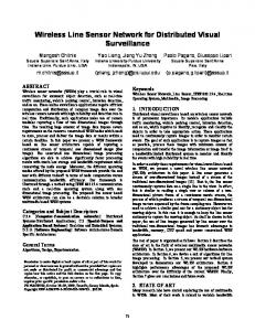
2. Overhead HV Transmission Power Networks-Multiconductor Transmission Line (MTL) Configurations and BPL Network Architecture 2.1. Overhead HV MTL Configurations. In the electrical power industry, overhead transmission systems are mainly classified by (i) their voltage levels, which may vary from 150 kV up to 1000 kV; (ii) the number of MTL circuits per each overhead HV tower. There are two main categories: single- and double-circuit MTL configurations. More specifically, in the case of single-circuit three-phase overhead HV configurations, each overhead HV tower supports threephase conductors. In the case of double-circuit three-phase overhead HV configurations, each overhead HV tower supports six-phase conductors; and (iii) the number of neutral conductors per each overhead HV tower [38–41]. A typical case of 150 kV single-circuit overhead HV MTL configuration is depicted in Figure 1. The three parallel phase kV are suspended conductors 1, 2, and 3 that are spaced by Δ150 𝑝

at heights ℎ𝑝150 kV above lossy ground on the overhead HV tower. Moreover, the two parallel neutral conductors 4 and kV hang at heights ℎ𝑛150 kV on 5 that are spaced by Δ150 𝑛 the overhead HV tower. This three-phase five-conductor overhead HV MTL configuration is considered in the present work consisting of ACSR GROSBEK conductors [40–43]. The exact dimensions of this overhead HV MTL configuration are detailed in [38, 41]. Depending on geographical constraints and other technoeconomic issues, the distance 𝐿 relay between two overhead HV towers varies from 0.5 km to 1 km. On signal propagation via overhead HV/BPL networks, the role of imperfect ground was analyzed in [38–41, 44– 52]. The ground is considered as the reference conductor. Its

ISRN Power Engineering

3 kV Δ150 n

4

1

rn150 kV

5

X

2

rp150 kV

3

kV Δ150 p

.. .

hp150 kV

hn150 kV

.. .

.. .

y

𝜀0 𝜇0

z x

𝜀 g𝜇 0 𝜎 g Phase conductor Neutral conductor

X Relay node Sensor

Figure 1: 150 kV single-circuit overhead HV MTL configuration integrated with WSN [38, 40–43].

conductivity 𝜎𝑔 is assumed equal to 5 mS/m while its relative permittivity 𝜀𝑟𝑔 is assumed equal to 13, which is a realistic scenario [38–41, 45, 47, 49]. 2.2. Overhead HV/BPL Networks and Corresponding HV/BPL Topologies. Today, thousands of km of overhead HV lines are installed in more than 120 countries. These lines stretch from the generation points to main consumers such as population centres and heavy industrial zones. These distances 𝐿 vary from approximately 25 km to 190 km. Shorter branch lengths 𝐿 in the range of 10 km to 50 km are used so that connections between overhead HV transmission lines can be deployed [38, 40, 41, 52–57]. Due to their ubiquitous nature, overhead HV lines define the cornerstone of developing an advanced IP-based power system, offering a plethora of potential SG applications [40, 41, 53, 54]. The transformation of the existing overhead HV power grid to a smarter overhead HV network can be achieved through the deployment of BPL networks across the existing power grid infrastructure. Apart from the delivery of broadband last mile access in remote and/or underdeveloped areas, overhead HV/BPL networks constitute a potentially convenient and inexpensive communication medium for the deployment of WSNs [31–37].

In overhead HV/BPL networks, the basic network device is the BPL unit. Depending on the BPL network design and the network performance requirements, BPL units that are installed onto overhead HV lines can be placed at distances 𝐿 BPL varying from 1 km to 100 km [38–41]. These units couple BPL signal into overhead HV lines via their integrated BPL modems. Each BPL unit can be configured either as repeater or as aggregator; a repeater performs extraction, regeneration, and injection of the BPL signal, whereas an aggregator collects the traffic generated by the BPL repeaters that are dispersed across the overhead HV/BPL network. Regardless of their role, each pair of adjacent BPL units defines the ends of a BPL subnetwork that is characterized by its topology [38, 40, 41, 58, 59]. Hence, each overhead HV/BPL network consists of the serial connection of different overhead HV/BPL topologies. Due to their system design, each BPL unit can comfortably support either wireless broadband access to end users, such as consumers and WSNs, through Bluetooth, ZigBee, and IEEE WiFi 802.11 technologies or wireless point-to-point connections to its adjacent BPL units [34–36]. Thus, the survivability of overhead HV/BPL networks with WSNs is guaranteed for several hours even if the wired connection of overhead HV lines between BPL units is temporarily

4 lost. Anyway, only the wireline communications interface between BPL units (BPL wireline connection) is examined in this paper. 2.3. Capacity of Overhead HV/BPL Networks. To examine the broadband potential of overhead HV/BPL networks, the exploitation of accurate channel models at high frequencies across the overhead HV lines is imperative. As usually done in BPL transmission, the hybrid method is employed to examine the spectral behavior of overhead HV/BPL networks installed on overhead HV MTL configurations [38–41, 44–48, 60– 63]. More specifically, the hybrid method, which is a careful cascade of well-known microwave engineering techniques, comprises (i) the bottom-up approach: it combines MTL theory with similarity transformations achieving to solve the propagation analysis problem by determining the excited modes of overhead HV MTL configurations in terms of their propagation constants; (ii) the top-down approach: it consists of the concatenation of multidimensional 𝑇-matrices that circuitally describe the transmission analysis problem across the occurred overhead HV/BPL topologies. Synoptically, the hybrid method receives as input the system parameters of the examined overhead HV MTL configurations and overhead HV/BPL topologies and gives as output a series of useful metrics, such as transfer function 𝐻(𝑓) and capacity 𝐶, that are suitable for assessing the broadband performance of overhead HV/BPL topologies and, thus, of overhead HV/BPL networks. Capacity is the maximum achievable transmission rate over an overhead HV/BPL channel. It depends on the overhead HV MTL configuration, the overhead HV/BPL topology, the operation frequency band, the applied coupling scheme that injects the BPL signal into overhead HV lines, the imposed injected power spectral density (IPSD) limits that regulate electromagnetic interference (EMI) emissions of the overhead HV/BPL network operation, and the noise characteristics. Therefore, to evaluate the capacity of overhead HV/BPL topologies, except for the transfer function, the hybrid method requires as additional inputs a set of related transmission and power spectral properties concerning the operation of overhead HV/BPL networks. In detail, these transmission and power spectral properties are as follows. (i) Coupling Scheme. According to how signals are injected onto overhead HV/BPL transmission lines, two different coupling schemes exist [39–41]: (i) wire-to-wire (WtW) coupling schemes when the signal is injected between two conductors; and (ii) wire-to-ground (WtG) coupling schemes when the signal is injected onto one conductor and returns via the ground. Without losing the generality of the analysis, only one WtG coupling scheme will be preferred for the rest of the analysis; with reference to Figure 1, only WtG coupling scheme between conductor 1 and ground is assumed (WtG1 coupling scheme). (ii) The IPSD Limits. Since overhead HV/BPL networks may become both a source and a victim of EMI, a critical issue related to their operation is the power constraints that should be imposed. These power constraints guarantee that

ISRN Power Engineering overhead HV/BPL networks harmonically coexist with other already licensed telecommunications systems [44, 47, 48, 64, 65]. Among regulatory bodies that have established EMI regulations concerning BPL network operation, the most important are those of FCC Part 15 due to their proneness to the broadband exploitation of BPL technology [66–70]. However, as it has already been presented in [39, 44, 47, 48], a simpler regulatory approach would be to avoid formal EMI compliance tests by limiting IPSD to a level that, in most circumstances, does not exceed the former EMI regulation. Among the different IPSD limit proposals that complied with FCC Part 15 limits, the IPSD limits proposed by Ofcom, which are detailed in [66–70], are the most cited. More specifically, for overhead HV/BPL networks, according to Ofcom, in the 3–30 MHz frequency range maximum levels of −60 dBm/Hz constitute appropriate IPSD limits 𝑝(𝑓) providing presumption of compliance with the current FCC Part 15 limits [39, 44, 47, 48, 70–72]. (iii) Noise Characteristics. According to [44, 47–49, 73– 76], two types of noise are dominant in overhead HV/BPL networks. (i) Colored background noise:it is the environmental noise that depends on weather conditions, humidity, geographical location, height of overhead HV MTL configuration, corona discharge, and so forth. (ii) Narrowband noise: it is the cumulative result of various narrowband interferences that are produced by other telecommunications systems operating at the same frequency range with overhead HV/BPL networks. In accordance with [39, 44], as it regards the noise properties of overhead HV/BPL networks in the 3–30 MHz frequency band, uniform additive white Gaussian noise (AWGN) PSD level 𝑁(𝑓) is assumed. Thoroughly examining the existing BPL noise literature [44, 47–49, 71– 73, 76], the average uniform AWGN/PSD level is equal to −105 dBm/Hz (average noise scenario). Taking into account the aforementioned power spectral and transmission properties, the capacity of an overhead HV/BPL topology in the 3–30 MHz frequency band is given by [39, 44, 47, 48, 77–79] as follows: 𝐿−1

𝐶 ≡ 𝐶 (𝐿 = 𝐾) = 𝑓𝑠 ∑ log2 {1 + [SNR (3 MHz + 𝑞𝑓𝑠 ) 𝑞=0

󵄨 󵄨2 ⋅󵄨󵄨󵄨𝐻 (3 MHz + 𝑞𝑓𝑠 )󵄨󵄨󵄨 ]} , (1) SNR (𝑓) = 𝐾=

⟨𝑝 (𝑓)⟩𝐿 , ⟨𝑁 (𝑓)⟩𝐿

(30 − 3) MHz , 𝑓𝑠

(2) (3)

where 𝐻{⋅} is the transfer function of the overhead HV/BPL topology considered that depends on the coupling scheme applied, ⟨⋅⟩𝐿 is an operator that converts dBm/Hz into a linear power ratio (W/Hz), 𝐾 is the number of subchannels in the BPL signal frequency range of interest, and 𝑓𝑠 is the flatfading subchannel frequency spacing.


5

The cumulative capacity is defined as the cumulative upper limit of information which can reliably be transmitted over the overhead HV/BPL topology. For given frequency 𝑓 ∈ [3, 30] MHz, overhead HVMTL configuration and coupling scheme configuration, taking into account (1), cumulative capacity is determined by [77–79] 󵄩󵄩 𝑓 − 3 MHz 󵄩󵄩 󵄩󵄩 󵄩 Cum 𝐶 (𝑓) = 𝐶 (𝐿 = 󵄩󵄩󵄩 󵄩󵄩 + 1) , 󵄩󵄩 󵄩󵄩 𝑓𝑠

(4)

where ‖𝑥‖ is the nearest integer to 𝑥. In fact, cumulative capacity describes the aggregate capacity effect of all subchannels of the examined frequency band.

3. WSNs across the Transmission Power Grid: WSN Communications Infrastructure and Network Models Since overhead HV networks can provide the necessary broadband communications platform for various SG applications, WSNs can be easily integrated in this broadband context [80, 81]. Based on an established mathematical framework suitable for describing WSNs of transmission power grids [11, 24–26, 82], WSN broadband performance as well as WSN coexistence with overhead HV/BPL networks is assessed through the performance metric of maximum delay time in delivering data measured by sensors [83–85]. 3.1. WSN Architecture. According to [11, 24–26], a WSN architecture tailor-made for supporting overhead HV line monitoring, metering, and controlling applications is depicted in Figure 1. Each overhead HV tower is equipped with a relay node that may have both short- and long-range communications capabilities depending on the functions of the relay nodes [14, 25]. The relay nodes receive data from their surrounding sensors, which can perform only short-range communication, that are located at overhead HV tower, overhead HV lines, and the surrounding environment [24, 86, 87]. Due to their long-range communications capabilities, relay nodes of adjacent overhead HV towers exchange the collected information between them [10]. The goal of this exchange is the arrival of collected information data to the control center or substations that define the ends of the overhead HV network—see Figures 2(a)–2(c). 3.2. Network Models. Network models help to tune the wireless and wireline communications infrastructure of the overhead HV lines so that WSN data are timely delivered to the control center. On the basis of the established mathematical framework of [11, 24–26], two well-validated models— that is, LNM and OANM—and the proposed one—that is, BPLeNM—are applied to WSNs with regard to the maximum delay time in delivering data measured by sensors to the control center (Internet); namely, we have the following. (i) LNM. As it has already been mentioned and depicted in Figure 2(a), the substations 1 and 2 define the ends of the examined overhead HV network. The substations are

connected to the control center via wireline connections, such as optical fibre, DSL connections, and Ethernet connections. The control center essentially allows the direct connection of WSNs with the Internet in order to allow their better supervision and control. In the following analysis, the delay time added by the connection of substations to the control center is omitted for all the examined network models due to these high-bitrate and short-length wireline connections. Depending on the length of the overhead HV network 𝐿 and the spacing between overhead HV towers 𝐿 relay , 𝑛relay = ⌈𝐿/𝐿 relay ⌉ − 1 overhead HV towers are distributed across the overhead HV network. Anyway, it is assumed that distance 𝐿 relay is a divisor of distance 𝐿 without harming the generality of the following analysis. Since each overhead HV tower is equipped with one relay node, 𝑛relay relay nodes are deployed across the overhead HV network. Each relay node receives the sent information from its surrounding sensors. Since sensors can perform only short-range communication links due to their battery restrictions and size, their communication with the relay node is achieved through short-range communication technologies, such as Bluetooth and ZigBee [19, 88, 89]. After collecting information from the sensors, the relay node wirelessly sends its information to its neighbor relay node that is closer to the substations. In Figure 2(a), this connection is denoted by sensor network wireless relaying. According to [11, 24–26], the maximum delay time, which is the total time for the data of the relay node ⌈𝑛relay /2⌉ to arrive at its nearest substation, is then given by

𝜏LNM =

⌈𝑛relay /2⌉ × (⌈𝑛relay /2⌉ + 1) × 𝑆𝑑 2𝑅SNWR

,

(5)

where ⌈𝑥⌉ returns the lowest integer that is not less than 𝑥, 𝑆𝑑 is the message size per relay node, and 𝑅SNWR is the data rate of the sensor network wireless relaying [90]. Note that the above simple calculation does not include the relaying channel access time and the data transmission time between sensors and relay node that are omitted for all the network models of this analysis. (ii) OANM. A more efficient network model to deliver the collected data from the sensors is the establishment of direct wireless links between relay nodes and the control center. With reference to Figure 2(b), these wireless links are denoted by long relay node wireless connections and permit the data exchange between relay nodes and Internet without the hopby-hop intervention of adjacent relay nodes and the existence of control center. Since base stations can be situated several km away from the relay nodes, the long relay node wireless connections should rely on cellular technologies, such as GSM, 3G, and 4G/LTE wireless connections [91]. Despite the delay and workload minimization, this network model is characterized by the high equipment cost and extra energy consumption due to the long relay node wireless connections. To establish a satisfactory trade-off between cost and delay minimization, OANM has been proposed in [11, 26]. According to this network model, 𝑔OANM relay nodes denoted by representative relay nodes are equipped with long relay

6


Control center (Internet)

Substation 1

1

Substation 2

2

3

nrelay −1

···

Relay node Relay node Relay node of pole 1 of pole 2 of pole 3

nrelay

Relay node Relay node of pole nrelay −1 of pole nrelay

(a) Control center (Internet)

Substation 1

1

Substation 2

2

···

irelay, OANM

···

irelay, OANM −

Relay node group G1

···

irelay, OANM +

nrelay

· · · nrelay −1

kOANM

2kOANM + 1 relay nodes Relay node group Gi𝑔

Relay node group Gg

OANM +2

OANM

(b) Control center (Internet)

Substation 1

1

···

2

···

kBPLeNM

···

Relay node group G1

irepeater

irelay, BPLeNM

···

···

irelay, BPLeNM + kBPLeNM

Substation 2

···

kBPLeNM + 1 relay nodes Relay node group Gi𝑔

BPLeNM

Wireline connection Sensor network wireless relaying Short relay node wireless connection

BPL wireline connection Long relay node wireless connection (c)

Figure 2: WSN architecture and network models (a) LNM, (b) OANM, and (c) BPLeNM.

ISRN Power Engineering node wireless connection capabilities. Also, the two substations are representative nodes because they are always connected to the Internet via wireline connections. The 𝑔OANM + 2 representative nodes define corresponding relay node groups where the 𝑛relay relay nodes of the overhead HV network are divided into these groups. In accordance with [11, 26], to determine the maximum delay time applying OANM, three assumptions should first be made. (i) Each relay node collects the same amount of data from its sensors. As it has already been mentioned, since the data transmission time between each sensor and relay node remains the same regardless of the network model applied, this time is neglected in the rest of this analysis. (ii) The maximum delay time of relay node groups is the same. This implies that each relay node group has a symmetric structure. With reference to , 𝑖𝑔OANM = Figure 2(b), each relay node group 𝐺𝑖𝑔 OANM 2, . . . , 𝑔OANM + 1, comprises 2𝑘OANM + 1 relay nodes. The middle relay node 𝑖, 𝑖 = 𝑖relay,OANM , is the representative one. The 2𝑘OANM relay nodes send their data in a hop-by-hop manner to the representative relay node as depicted in Figure 2(b). (iii) The remaining 𝑛relay − 𝑔OANM × (2𝑘OANM + 1) relay , nodes are divided into the node groups 𝐺𝑖𝑔 OANM 𝑖𝑔OANM = 1, and 𝐺𝑖𝑔 , 𝑖𝑔OANM = 𝑔OANM + 2, of OANM the substations 1 and 2, respectively. With reference to Figure 2(b), the relay nodes 𝑖, 𝑖 = 1, . . . , ⌈(𝑛relay − 𝑔OANM × (2𝑘OANM + 1))/2⌉, send their data in a hopby-hop manner to the substation 1, whereas the relay nodes 𝑖, 𝑖 = 𝑛relay − ⌊(𝑛relay − 𝑔OANM × (2𝑘OANM + 1))/2⌋ + 1, . . . , 𝑛relay , send their data in a hop-byhop manner to the substation 2 where ⌊𝑥⌋ returns the largest integer not greater than 𝑥. Hence, the maximum delay time of the node group of substation 1 is always greater or equal in comparison with the maximum delay time of the node group of substation 2.

7 maximum delay time of the relay node is determined by (1) = 𝜏OANM,RNG

𝑘OANM × (𝑘OANM + 1) × 𝑆𝑑 𝑘OANM × 𝑆𝑑 + . 2𝑅SNWR 𝑅SNWR (6)

Note that the last term in (6) represents the delay time that one side of the relay node group should wait so that no collision occurs in the representative relay node due to the simultaneous transmission of the other side; (b) the delay time of sending all the collected data from the representative relay node to the control center through the long relay node (2) . This delay time is wireless connection 𝜏OANM,RNG given from (2) = 𝜏OANM,RNG

(2𝑘OANM + 1) × 𝑆𝑑 , 𝑅LRNWC

(7)

where 𝑅LRNWC is the data rate of the long relay node wireless connection. The maximum delay time of the relay node group is determined from (1) (2) 𝜏OANM,RNG = 𝜏OANM,RNG + 𝜏OANM,RNG .

(8)

(ii) The Maximum Delay Time of the Node Group of Substation 1 𝜏OANM,NG1 . It is the total time for the data of the relay node ⌈(𝑛relay − 𝑔OANM × (2𝑘OANM + 1))/2⌉ to arrive at the substation 1. Based on (5), the maximum delay time of the node group of substation 1 is determined by 𝜏OANM,NG1 = (⌈

𝑛relay − 𝑔OANM × (2𝑘OANM + 1) 2 × (⌈

⌉

𝑛relay − 𝑔OANM × (2𝑘OANM + 1) 2

⌉ + 1) × 𝑆𝑑 )

−1

To evaluate the maximum delay time, two other delay times should previously be determined; namely, we have the following. (i) The Maximum Delay Time of the Relay Node Group 𝜏OANM,RNG . Since all relay node groups have the same long relay node wireless connection capabilities and the same symmetric structure with equal number of relay nodes, these relay node groups present the same maximum delay time. With reference to Figure 2(b), there are two components in the delay, namely: (a) (1) , the maximum delay time of the relay node 𝜏OANM,RNG which is the total time for the data of the relay node 𝑖relay,OANM + 𝑘OANM to arrive to its corresponding representative relay node 𝑖relay,OANM . Based on (5), the

× (2𝑅SMWR ) . (9) Taking into account (8) and (9), the maximum delay time is determined from 𝜏OANM = max {𝜏OANM,RNG , 𝜏OANM,NG1 } ,

(10)

where max{𝑥, 𝑦} returns the highest value between either 𝑥 or 𝑦. In [11, 16, 20, 26, 92], the optimization problem of minimizing the maximum delay time of (10) has been investigated. More specifically, the optimization problem of OANM determines the value of parameters such as the number of long relay node wireless connections and the number of relay nodes per each node group for given overhead HV network

8


and cost/energy restrictions. In addition, straightforward relations among the former parameters and the maximum delay time in information delivery have been presented. (i) BPLeNM: based on the architecture of overhead HV/BPL networks, the proposed network model exploits the already validated knowledge of LNM and the OANM. More specifically, overhead HV lines cover distances 𝐿 that vary from 10 km to 190 km, whereas BPL units that are installed onto these lines can be placed at distances 𝐿 BPL varying from 1 km to 50 km [38–42, 53–57]. Depending on the previous distances, 𝑛BPL = ⌈𝐿/𝐿 BPL ⌉ − 1, BPL units are installed across the overhead HV network. To facilitate the following analysis without harming its generality, it is assumed that distances 𝐿 BPL and 𝐿 relay are divisors of distances 𝐿 and 𝐿 BPL , respectively. Hence, the assumption of LNM indicating that the distance 𝐿 relay is a divisor of distance 𝐿 is also valid in BPLeNM. Anyway, the previous assumptions can be easily implemented during the design of overhead HV/BPL networks. In order to validate the mathematical model and the maximum delay time of BPLeNM, four assumptions concerning the network architecture of BPLeNM are given. (a) Each relay node collects the same amount of data from its sensors. (b) The maximum delay time of relay node groups is the same. This implies that each relay node group has a symmetric structure. With reference to Figure 2(c), each relay node group 𝐺𝑖𝑔BPLeNM , 𝑖𝑔BPLeNM = 2, . . . , 𝑔BPLeNM + 1, comprises 𝑘BPLeNM + 1 relay nodes. The first relay node 𝑖, 𝑖 = 𝑖relay,BPLeNM , of the relay node group is the representative one. The other 𝑘BPLeNM relay nodes send their data in a hopby-hop manner to the representative relay node as depicted in Figure 2(c). When the representative relay node receives all the data, then it sends them to the corresponding 𝑖repeater BPL unit via a short relay node wireless connection, such as Bluetooth, ZigBee, or IEEE WiFi 802.11 technology. Today, IEEE WiFi 802.11 technology is the most common interface of BPL units [58, 59]. (c) After collecting information from the representative relay node, the BPL unit sends its information to its neighbor BPL unit, that is, closer to the substations. In Figure 2(c), this information delivery is achieved through the BPL wireline connection in a hop-by-hop manner. Similarly to LNM, BPL units 𝑖repeater = 1, . . . , ⌈𝑛BPLeNM /2⌉ send their collected data to the substation 1, whereas BPL units 𝑖repeater = ⌈𝑛BPLeNM /2⌉ + 1, . . . , 𝑛BPLeNM send their collected data to the substation 2. (d) The remaining 𝑛relay − 𝑔BPLeNM × (𝑘BPLeNM + 1) relay nodes are allocated to the node group 𝐺𝑖𝑔BPLeNM , 𝑖𝑔BPLeNM = 1, of the substation 1. With reference to Figure 2(c), the relay nodes 𝑖, 𝑖 = 1, . . . , 𝑘BPLeNM , send their data in a hop-by-hop manner to the substation 1. Conversely to OANM, 𝑘BPLeNM is not a user-defined

variable but it depends on the distances 𝐿 BPL and 𝐿 relay through the relation 𝑘BPLeNM = ⌈𝐿 BPL /𝐿 relay ⌉ − 1. To evaluate the maximum delay time, two other delay times should previously be determined; namely, we have the following. (i) The Maximum Delay Time of the Relay Node Group via BPL Units 𝜏BPLeNM,RNG . Since all relay node groups have the same short relay node wireless connection capabilities either between them or to the BPL units and the same symmetric structure with equal number of relay nodes, these relay node groups present the same maximum delay time. With reference to Figure 2(c), there are three components in the delay, namely: (a) the maximum delay time of the relay node (1) , which is the total time for the data of 𝜏BPLeNM,RNG the relay node 𝑖relay,BPLeNM + 𝑘BPLeNM to arrive to its corresponding representative relay node 𝑖relay,BPLeNM . Similarly to (6), the maximum delay time of the relay node is determined by (1) = 𝜏BPLeNM,RNG

𝑘BPLeNM × (𝑘BPLeNM + 1) × 𝑆𝑑 . 2𝑅SNWR

(11)

In contrast with (6), only one side in the relay node group exists. Thus, no collision occurs in the representative relay node; (b) the delay time of sending all the collected data from the representative relay node to the BPL unit through the short relay node wireless (2) . This delay time is given from connection 𝜏BPLeNM,RNG (2) = 𝜏BPLeNM,RNG

(𝑘BPLeNM + 1) × 𝑆𝑑 , 𝑅SRNWC

(12)

where 𝑅SRNWC is the data rate of the short relay node wireless connection; and (c) the maximum delay time (3) , which is the total time of the BPL unit 𝜏BPLeNM,RNG for the data of the BPL unit 𝑖repeater to arrive to the substation. Similarly to (6), the maximum delay time, which is the total time for the data of the BPL unit ⌈𝑛BPL /2⌉ to arrive at its nearest substation, is then given by (3) = 𝜏BPLeNM,RNG

⌈𝑛BPL /2⌉×(⌈𝑛BPL /2⌉ + 1)×(𝑘BPLeNM + 1)×𝑆𝑑 , 2𝑅BPL (13)

where 𝑅BPL is the data rate of the BPL wireline connection. In accordance with Section 2.2, capacity is the maximum achievable transmission rate over an overhead HV/BPL channel. Thus, data rate 𝑅BPL is equal to or lower than the capacity of the arisen overhead HV/BPL topology between two adjacent BPL units or one BPL unit and the substation; say 𝑅BPL ≤ 𝐶. The maximum delay time of the relay node group is determined from (1) (2) (3) + 𝜏BPLeNM,RNG + 𝜏BPLeNM,RNG . 𝜏BPLeNM,RNG = 𝜏BPLeNM,RNG (14)


9

(ii) The Maximum Delay Time of the Node Group of Substation 1 𝜏BPLeNM,NG1 . It is the total time for the data of the relay node 𝑘BPLeNM to arrive at the substation 1. Based on (9), the maximum delay time of the node group of substation 1 is determined by 𝜏BPLeNM,NG1 =

𝑘BPLeNM × (𝑘BPLeNM + 1) × 𝑆𝑑 . 2𝑅SNWR

(15)

Taking into account (14) and (15), the maximum delay time is given from 𝜏BPLeNM = max {𝜏BPLeNM,RNG , 𝜏BPLeNM,NG1 } .

(16)

From (16), it is evident that the maximum delay time of BPLeNM mainly depends on the design of overhead HV/BPL network, say, the number of BPL units.

4. Numerical Results and Discussion The simulation results of various implementation scenarios of WSNs and overhead HV networks aim at highlighting (i) their broadband performance and how various inherent and imposed factors influence the metric of maximum delay time; (ii) the comparative performance of LNM, OANM, and the proposed BPLeNM for a plethora of different arrangement scenarios. All the system parameters as well as their default values that are involved in the following analysis are reported in Table 1. These values help towards the establishment of realistic implementation scenarios. Note that all the assumptions of Section 3.2 are satisfied. 4.1. Influence of Overhead HV/BPL Topologies on BPL Capacity Performance. The capacity performance of overhead HV/BPL networks in terms of capacity and cumulative capacity is evaluated based on the application of FCC Part 15 limits and the assumption of average noise scenario in the 3–30 MHz frequency band. In this subsection, the impact of the length of overhead HV/BPL topologies on the capacity metrics of Section 2.3 is examined. For the numerical computations, the 150 kV single-circuit overhead HV MTL configuration, depicted in Figure 1, has been considered. In order to apply the BPLeNM, an overhead HV/BPL network of length 𝐿 is divided into 𝑛BPL +1 overhead HV/BPL topologies of length 𝐿 BPL . Each overhead HV/BPL topology is separated into segments—network modules— each of them comprising the successive branches encountered, see Figure 3. However, this paper only focuses on overhead HV/BPL networks that comprise “LOS” transmission topologies where “LOS” topologies correspond to line-ofsight transmission of wireless channels (i.e., no branches are encountered, 𝐿 𝑏1 = 𝐿 𝑏2 = ⋅ ⋅ ⋅ = 𝐿 𝑏𝑛BPL+1 = 0, 𝑍𝑏1 = 𝑍𝑏2 = ⋅ ⋅ ⋅ = 𝑍𝑏𝑛BPL+1 = ∞). Hence, the “LOS” transmission along the average end-to-end distance 𝐿 BPL of the overhead HV/BPL topology is assumed. With reference to Figure 3, the transmitting and the receiving ends are assumed matched to the characteristic impedance of the supported channels, which is a typical procedure [39–42, 44–49, 55].

With reference to Figure 3 and Table 1, six indicative overhead HV/BPL topologies of “LOS” transmission are examined; namely, we have the following. (1) The “LOS” transmission along the distance 𝐿 BPL = 1 km (topology A). (2) The “LOS” transmission along the distance 𝐿 BPL = 2 km (topology B). (3) The “LOS” transmission along the distance 𝐿 BPL = 5 km (topology C). (4) The “LOS” transmission along the distance 𝐿 BPL = 10 km (topology D). (5) The “LOS” transmission along the distance 𝐿 BPL = 25 km (topology E). (6) The “LOS” transmission along the distance 𝐿 BPL = 50 km (topology F). As it concerns the capacity characteristics of the 150 kV single-circuit overhead HV/BPL topologies, in Figure 4, the cumulative capacity is plotted versus frequency in the 3– 30 MHz frequency band for topologies A, B, C, D, E, and F. Observing Figure 4, the following are clearly demonstrated. (i) The simulation results of typical-length “LOS” transmission topologies indicate the potentially excellent communications medium of overhead HV/BPL networks. Already verified in [39–42, 44, 47, 48], the entire overhead transmission power grid resembles a flat-fading transmission system with low-loss and high-capacity characteristics providing an attractive broadband communications platform for various SG applications such as WSNs [93]. (ii) Regardless of the overhead HV/BPL topology, the low-loss flat-fading transmission system with highcapacity characteristics still exists. Although end-toend overhead HV topologies of lengths up to 50 km are examined, the corresponding capacity results are very encouraging in the 3–30 MHz frequency band when FCC Part 15 limits and average noise scenario are considered; that is, when the distance 𝐿 BPL is equal to 1 km, 2 km, 5 km, 10 km, 25 km, and 50 km, the capacity 𝐶 of the overhead HV/BPL topology is equal to 393 Mbps, 382 Mbps, 345 Mbps, 317 Mbps, 269 Mbps, and 224 Mbps, respectively. (iii) The previous capacity results reveal the critical role of distance between BPL units during the design of overhead HV/BPL networks. The high number of BPL units implies that overhead HV/BPL topologies are characterized by shorter end-to-end distances 𝐿 BPL permitting higher capacities for the overhead HV/BPL network. Nonetheless, denser overhead HV/BPL topologies require higher network infrastructure complicacy and higher time delay due to the hop-by-hop manner of wireline communications relaying. It is evident that there is a trade-off between the capacity and the time delay that is analytically investigated in Section 4.2.3.

10


Transmitting End

BPL unit 1

BPL unit 2

BPL unit nBPL

A L BPL

L BPL

L BPL

B

Receiving End

L BPL

L

L b1 Matched input termination

Zb1

L b2 X

Zb2

X···X

Z2 L BPL

Z1 L BPL

L b𝑛

Zb𝑛

L b𝑛

BPL

BPL

ZnBPL L BPL

ZbBPL +1 BPL

+1

X ZnBPL +1 L BPL

Matched output termination

Figure 3: An indicative overhead HV/BPL network considered as a cascade of 𝑁 + 1 modules corresponding to 𝑁 + 1 overhead HV/BPL topologies. Table 1: System parameters of the used WSNs and overhead HV/BPL topologies. Length of the 1, 2, 5, 10, overhead HV 25, 50, 100 network L (km)

Distance 1, 2, 5, 10, 25, between BPL 50 units LBPL (km)

Distance between relay nodes Lrelay (km)

Message size per relay node 𝑆𝑑 (kbps)

0.5, 1

32, 64, 128

Data rate of the sensor network wireless relaying RSNWR (kbps)

64 kbps Data rate of the (GSM), Data rate of the long relay node 384 kbps (3G), BPL wireline wireless 20 Mbps connection RBPL connection RLRNWC (4G/LTE)

RBPL ≤ 𝐶

different arrangements of the three network models (i.e., LNM, OANM, and BPLeNM) are adopted. The impact of various parameters, such as distance between relay nodes 𝐿 relay , distance between BPL units 𝐿 BPL , message size per relay node 𝑆𝑑 , data rate of the long relay node wireless connection 𝑅LRNWC , data rate of the short relay node wireless connection 𝑅SRNWC , data rate of the BPL wireline connection 𝑅BPL , and different ICTs on maximum time daily is thoroughly studied.

500

Cumulative capacity (Mbps)

250 (ZigBee)

780 kbps Data rate of the (Bluetooth), short relay node 250 kbps (ZigBee), wireless 54/11 Mbps (IEEE connection WiFi 802.11a/b) RSRNWC

400

300

200

Figure 4: Cumulative capacity of the 150 kV single-circuit overhead HV MTL configuration versus frequency for different “LOS” transmission topologies when FCC Part 15 limits and average noise scenario are considered and WtG1 coupling scheme is applied (for plot clarity reasons, the subchannel frequency spacing is equal to 1 MHz).

4.2.1. LNM. After the consideration of its mathematical analysis in Section 3.2, LNM is the simpler and the more intuitive network model for describing the behaviour of WSNs across overhead HV networks. It is characterized by clarity and a straightforward examination of the information delivery problem while the computation of maximum delay time is synopsized by only one equation—see (3). However, the cost of simplicity, which is highlighted in this subsection, is the poor performance in terms of maximum delay time. In Figure 5(a), the maximum delay time of LNM is plotted versus the length of the overhead HV network for different message sizes per relay node when the distance between relay nodes is equal to 0.5 km. In Figure 5(b), same curves are given but for distance between relay nodes equal to 1 km. From Figures 5(a) and 5(b), several interesting remarks regarding LNM performance can be highlighted.

4.2. Maximum Delay Time and Network Models. The following discussion focuses on the maximum delay time of WSNs that are deployed across overhead HV networks when

(i) Depending on geographical constraints and other technoeconomic issues, the distance between two overhead HV towers, which is equal to the distance between relay nodes, can vary from 0.5 km to 1 km.

100

0 0

5

Topology A Topology B Topology C

20 10 15 Frequency (MHz)

25

30

Topology D Topology E Topology F

11

3000

Maximum delay time (s)



2000 1000 0

0

20 40 60 80 Length of the overhead HV network (km)

100

Sd = 32 kbits Sd = 64 kbits Sd = 128 kbits

800 600 400 200 0

0


100


(a)

(b)

Figure 5: Maximum delay time of the 150 kV single-circuit overhead HV MTL configuration versus length of the overhead HV network for different message sizes per relay node. (a) Distance between relay nodes 𝐿 relay = 0.5 km. (b) Distance between relay nodes 𝐿 relay = 1 km.

Shorter distances between overhead HV towers imply denser WSNs and higher requirements for WSN data delivery [17, 23, 30, 94, 95]. Observing (5) and Figures 5(a) and 5(b), doubling the number of relay nodes causes quadrupling of the maximum delay time. (ii) WSNs have gained attention for power grids due to their collaborative, convenient, and environmentfriendly nature. Their adoption and further exploitation will continue because they offer a reliable and efficient management of critical power grid pieces of equipment [6, 17, 23, 96, 97]. However, the implementation of denser WSNs will create an increase of the gathered information that implies a respective increase of message size per relay node. Taking into consideration (5) and Figures 5(a) and 5(b), doubling the size of WSN per relay node creates doubling of the maximum delay time. (iii) Apart from the delay issue, LNM suffers from imbalance of workload. The traffic handled by the relay nodes that are closer to the substations is significantly higher than the traffic served by the relay nodes that are installed farther away [11]. 4.2.2. OANM. The maximum delay time results of Section 4.2.1 indicate that LNM is suitable for overhead HV networks that are characterized by short end-to-end distances and low demands for monitoring and surveillance. Otherwise, the occurred delay times are prohibitive for real-time operations across the overhead HV network. In fact, the previous conditions can only be identified in areas where branches of overhead HV networks are deployed. Due to these findings, it is necessary to identify a more efficient and robust network model in order to deliver the gathered sensor data. With reference to Figure 2(b), through the establishment of long relay node wireless connections between representative relay nodes and the control center, OANM succeeds in sending the collected sensor data of relay nodes to the control center directly without relying on neighbor relay nodes [11, 16, 20, 26, 92]. In OANM, the number of relay node

groups as well as the number of the allocated relay nodes per group is adjusted in accordance with the WSN performance requirements. In Figure 6(a), the maximum delay time is plotted versus the number of relay node groups and the number of relay nodes per relay node group for a 100 km long overhead HV network. GSM technology is used for the long relay node wireless connections; the message size per relay node is assumed to be equal to 32 kbits and the distance between relay nodes is equal to 1 km. In Figures 6(b) and 6(c), same plots are given when 3G and 4G/LTE technologies are adopted for the long relay node wireless connections, respectively. Studying Figures 6(a)–6(c), several interesting findings concerning the performance of OANM can be pointed out; namely, we have the following. (i) The increase of the number of relay node groups reduces the maximum delay time. This is due to the fact that the information data of sensors prefer to be transferred via the fast long relay node wireless connections instead of stacking during the hop-byhop manner of short relay node wireless connections. However, the trend of maximum delay time shows a diminishing return; when the number of relay node groups is above 80% of the total relay nodes, the potential maximum delay time improvement is small. The best result concerning the maximum delay time is achieved when each relay node has long relay node wireless connection capabilities; for the 100 km long overhead HV network, the maximum delay time is equal to 0.5 s, 0.083 s, and 0.0016 s for GSM, 3G, and 4G/LTE transmission technologies, respectively. (ii) If the number of relay node groups is relatively small (i.e., below 20% of the total relay nodes), then more relay nodes per group are required so that the maximum delay time remains lower than the respective one of LNM. In fact, when there is no long relay node wireless connection (i.e., the relay node group is equal to zero), the maximum delay time of OANM coincides with the respective one of LNM. All the WSN information data are transmitted through

12


250



250

200 150 100 50 s 0 up 0 gro e d 0 50 no ay Numb l 50 e er of re fr lay n 100 100 er o node g odes per rela b m roup y Nu

200 150 100 50 s 0 up 0 gro e d 0 50 no ay Numb l 50 e er of re fr lay n 100 100 er o node g odes per rela b m roup y Nu

(a)

(b)


250

200 150 100 50 0 ps 0 rou g e 0 od 50 yn a Numb l 50 er of re f re lay n 100 100 er o node g odes per rela b m roup y Nu (c)

Figure 6: Maximum delay time of the 150 kV single-circuit overhead HV MTL configuration of topology F for different relay node group arrangements. (a) GSM. (b) 3G. (c) 4G/LTE.

the short relay node wireless connections using the LNM hop-by-hop manner.

time of OANM is worse than the respective one of LNM.

(iii) The worst case scenario in terms of the maximum delay time occurs when only one relay node group is used. Actually, when the relay nodes that are allocated to this relay node group are greater than 50% of the total relay nodes, all the gathered information arrives at the representative relay node in a hop-byhop manner creating an information stack. The worst maximum delay time occurs when only one relay node group is deployed and all the relay nodes of WSN are put into this group; for the 100 km long overhead HV network, the maximum delay time is equal to 213 s, 171 s, and 163 s for GSM, 3G, and 4G/LTE transmission technologies, respectively. Despite the used transmission technology, the maximum delay

(iv) For the same number of relay node groups, 4G/LTE and 3G transmission technologies show a slightly smaller maximum delay time than that of GSM [91, 98]. In fact, the main performance improvements occur in the best and worst cases because the information transmission of these cases is mainly based on the long relay node wireless connection. (v) To have schedulable and practically feasible relay node group arrangements, there is an additional physical constraint on how many relay nodes can be allocated into a relay node group. Since sensors periodically generate data—that is, the average reporting interval time of sensors is equal to 4 s—the data rate of the long relay node wireless connections should

ISRN Power Engineering be faster than the sensor data generation rate within a group. Otherwise, data will be backlogged creating an overflow at buffer of the representative relay node (backlog problem). In accordance with [11], GSM technology poses significant restrictions regarding the size of the relay node group arrangements. Also taking into consideration the previous assumption concerning the performance of various transmission technologies, only 3G transmission technology is going to be considered, hereafter. (vi) In order to minimize the maximum delay time and balance the workload among relay nodes, each relay node should have a direct wireless link to the control center. Despite its promising results, this arrangement is expensive in terms of equipment costs, deployment costs, maintenance costs, and extra energy consumption due to the direct cellular wireless links [11, 16, 92]. Apart from the worst and best cases, an average arrangement should be selected; the arrangement that presents maximum delay time equal to the median value of the maximum delay time defines a macroscopic metric providing a more representative estimate of the performance results of OANM. With respect to Figure 6(a) and for the 100 km long overhead HV network, when two relay node groups with 49 relay nodes each are deployed, the maximum delay time is equal to 45.6 s, that is, the median value of maximum delay time. Anyway, this high value of the maximum delay time of the average arrangement in comparison with the reporting interval time reveals that arrangements near to the best case should be implemented in order to successfully cope with the backlog problem. Without losing the generality of the analysis, only the worst, the average, and the best cases of OANM are considered in the following analysis. Similarly to LNM, OANM is thoroughly studied when different scenarios concerning the future expansion of WSNs across overhead HV networks occur. More specifically, in Figure 7(a), the maximum delay time is plotted versus the length of the overhead HV network for different message sizes per relay node when the distance between relay nodes is equal to 0.5 km and the worst case of OANM is adopted. In the same figure, the reporting interval time is also depicted. In Figures 7(b) and 7(c), the same curves are drawn for the average and the best case of OANM, respectively. In Figures 7(d)–7(f), the same plots with Figures 7(a)–7(c) are given when the distance between relay nodes is equal to 1 km. From Figures 7(a)–7(f), the following are obvious. (i) Regardless of the arrangement and the message size per relay node, OANM succeeds in maintaining the maximum delay time of overhead HV networks lower than the reporting interval time when their end-toend distance is lower than 10 km. To maintain the maximum delay time under the limit of the reporting interval time for distances higher than 10 km, WSN arrangements near to the best case should be implemented.

13 (ii) The influence of shorter distances between relay nodes and of the increase of message size per relay node on the OANM maximum delay time remains the same when bad and average cases of OANM are applied. Conversely, the previous changes have little impact on the maximum delay time of the best case. Since the best case of OANM mainly depends on the transmission through long relay node wireless connections, the changes that occur in the wireline environment leave intact the maximum delay time that is significantly lower than the limit of the reporting interval time in any case. (iii) To secure the future expansion of SG and WSNs, a technically viable solution is the installation of the best case of OANM. Significant problems of this proposal are the aforementioned issues related with the high installation and maintenance cost and certain assumptions dealing with the operation of the network model. More specifically, OANM heavily relies on symmetry; WSN communications infrastructure, long relay node wireless connection infrastructure, and all representative relay nodes are assumed to be symmetric and available at all times. However, a plethora of factors can bring in asymmetry OANM destabilizing its performance metrics [16, 92]. 4.2.3. BPLeNM. The maximum delay time results of Sections 4.2.1 and 4.2.2 reveal that the existing network models are confined to offer reliable monitoring and control services only to overhead HV networks that are characterized by short end-to-end distances and low demands for monitoring and surveillance. At the same time, the cost of securing abundant WSN broadband services to the future’s overhead HV networks is rather prohibitive; to cover the broadband needs of multi-km overhead HV networks with the existing network models, each relay node should be upgraded with long relay node wireless connection capabilities. However, this upgrade skyrockets the overall investment cost. Due to these findings, it is obligatory to exploit a rather more hard-hitting network model that can significantly reduce the maximum delay time below the limit of the reporting interval time and, at the same time, maintain a decent and affordable cost. In Section 4.1, it has been highlighted the excellent broadband potential of overhead HV/BPL networks. Actually, overhead HV/BPL networks are already installed in many countries worldwide and can provide the broadband communications platform for the implementation of WSNs. Through the exploitation of the installed BPL units across the overhead HV network, representative relay nodes can have a broadband access to the control center. In contrast with OANM, the BPL units that are already deployed onto the overhead HV lines straightforwardly define the number of the allocated relay nodes per each BPL unit. The proposed BPLeNM gives a clear broadband view to the problem of monitoring and surveillance of overhead HV networks using WSNs.

14




2500 2000 1500 1000 500 0

4 Maximum delay time (s)

800

3000

600 400 200 0

100 0 50 Length of the overhead HV network (km)

(c)

4

400 300 200 100 0

0 50 100 Length of the overhead HV network (km) Sd = 32 kbits Sd = 64 kbits Sd = 128 kbits





200

500

1

(b)

700 600

2

0


(a)

3

150 100 50 0


(d)

(e)

3 2 1 0


(f)

Figure 7: Maximum delay time of the 150 kV single-circuit overhead HV MTL configuration versus length of the overhead HV network for different message sizes per relay node as well as the reporting interval time (the yellow line). (a) Worst case of OANM, distance between relay nodes 𝐿 relay = 0.5 km. (b) Average case of OANM, distance between relay nodes 𝐿 relay = 0.5 km. (c) Best case of OANM, distance between relay nodes 𝐿 relay = 0.5 km. (d) Worst case of OANM, distance between relay nodes 𝐿 relay = 1 km. (e) Average case of OANM, distance between relay nodes 𝐿 relay = 1 km. (f) Best case of OANM, distance between relay nodes 𝐿 relay = 1 km.

In Figure 8(a), the capacity of the arisen overhead HV/BPL topologies is plotted with respect to the number of BPL units when a 100 km long overhead HV network is considered; FCC Part 15 limits are adopted and average noise scenario is assumed in the 3–30 MHz frequency band. In Figure 8(b), the maximum delay time is plotted versus the number of BPL units and the data rate of the BPL wireline connections for the same overhead HV network. Bluetooth technology is used for the short relay node wireless connections, ZigBee technology is applied for the sensor network wireless relaying connections, and the message size per relay node is assumed to be equal to 32 kbits while the distance between relay nodes is equal to 1 km. In Figures 8(c), 8(d), and 8(e), the same curves with Figure 8(b) are drawn when ZigBee, IEEE WiFi 802.11a, and IEEE WiFi 802.11b technologies are used for the short relay node wireless connections, respectively. Note that the data rates of the arisen overhead HV/BPL topologies are lower than or equal to their respective capacities. Also, in this paper, the minimum data rate of the BPL wireline connections is assumed equal to 1 Mbps while the respective data rate sampling is assumed equal to 5 Mbps.

From Figures 8(a)–8(e), important conclusions regarding the broadband operation and performance of overhead HV/BPL networks and WSNs are deduced; namely, we have the following. (i) Except for (i) the overhead HV/BPL topologies F and E that correspond to one and three BPL units; (ii) the cases of data rates of the BPL wireline connections lower than 1 Mbps, the maximum delay time of BPLeNM is extremely low in all the other cases examined regardless of the data rate of BPL wireline connections and the short relay node wireless connection technology applied. Actually, this result becomes evident because the arisen overhead HV/BPL topologies are characterized by significantly higher data rates in comparison with the sensor network wireless relaying technologies. Due to this broadband information platform, the maximum delay time mainly depends on the delay time of hop-by-hop relaying inside the relay node groups. (ii) The maximum delay time of BPLeNM mainly depends on the maximum delay time of the relay node


15

400


380 Capacity (Mbps)

360 340 320 300 280 260

20 40 Num 60 ber of B 80 PL 100 uni ts

240 220 0

10

20

30

40 50 60 70 Number of BPL units

80

90

180 160 140 120 100 80 60 40 20 0 0

100

(b)



(a)

180 160 140 120 100 80 60 40 20 0 0


0

0

400 300 350 200 250 150 e irelin 50 100 e BPL w te of th (Mbps) a r ta a D ons connecti

300 350 200 250 150 ireline 50 100 e BPL w th f o te Data ra nections (Mbps) con

400

160 140 120 100 80 60 40 20 0 0


(d)


(c)

0

400 300 350 200 250 150 e irelin 50 100 e BPL w te of th (Mbps) a r ta a D ons connecti

160 140 120 100 80 60 40 20 0 0


0

350 250 300 150 200 ne 100 li 50 PL wire of the B bps) te a r Data nections (M con

400

(e)

Figure 8: (a) Capacity of the overhead HV/BPL topologies for the 100 km long overhead HV network. (b, c, d, e) Maximum delay time versus the number of BPL units and the data rate of BPL wireline connections for the 100 km long overhead HV network: (b) Bluetooth short relay node wireless connections. (c) ZigBee short relay node wireless connections. (d) IEEE WiFi 802.11a short relay node wireless connections. (e) IEEE WiFi 802.11b short relay node wireless connections.

group via BPL units. This is due to the fact that the maximum delay time of the relay node group via BPL units is greater than the maximum delay time of the node group of substation 1 in all the arrangements examined. This is rather obvious investigating either (16) or Figure 2(c). (iii) The influence of different short relay node wireless connection technologies, such as Bluetooth, ZigBee, and IEEE WiFi 802.11, is negligible on the maximum

delay time. Since the number of relay nodes per relay node group is low, the generated information is also low. Therefore, the delay that is added at this information transmission stage is approximately equal to the delay that is added due to the insertion of one additional relay node. In the following analysis, only IEEE WiFi 802.11a technology, which is the most widely used wireless broadband access interface in BPL technology, is applied.

16

ISRN Power Engineering (iv) Capacity is the maximum achievable transmission rate over an overhead HV/BPL topology having a rather theoretical value. Even if the data rate of BPL wireline connections is limited to a small fraction of the capacity (e.g., 5%–10% of the capacity), the maximum delay time is well below the limit of the reporting interval time. Anyway, the significant remaining bandwidth of overhead HV/BPL networks validates the strong potential of overhead HV networks to support various SG applications and broadband access from consumers to remote and underdeveloped areas (last mile access problem) [34–37]. (v) Similarly to OANM, an average arrangement should be selected apart from the worst and best case. The arrangement that presents maximum delay time equal to the median value of the maximum delay time defines a representative estimate of the BPLeNM performance. When IEEE WiFi 802.11a is deployed for the short relay node wireless connection, the following worst, average, and best cases of the typical 100 km long overhead HV network are defined. (a) The worst maximum delay time is equal to 158 s when 1 BPL unit is installed across the 100 km long overhead HV network and the data rate of the BPL wireline connections is equal to 1 Mbps (low capacity bound of the BPL operation). (b) The average maximum delay time is equal to 1.37 s when 19 BPL units are installed across the 100 km long overhead HV network and the data rate of the BPL wireline connections is equal to 6 Mbps. (c) The best maximum delay time is equal to 0.105 s when 99 BPL units are installed across the 100 km long overhead HV network and the data rate of the BPL wireline connections is equal to the capacity (393 Mbps for the 100 km long overhead HV network). (vi) Comparing the worst, the average, and the best maximum delay time of BPLeNM with the respective ones of OANM and LNM for 100 km long overhead HV networks, the advantage of BPLeNM is clearly highlighted. (a) The worst maximum delay time of BPLeNM is equal to 158 s while the respective ones of OANM and LNM are equal to 163 s (4G/LTE technology) and 163 s, respectively. (b) The differences of average maximum delay times between the three network models are significant: BPLeNM delay time is equal to 1.37 in contrast with OANM and LNM delay times that are equal to 45.6 s and 163 s, respectively. Only BPLeNM succeeds in maintaining the average delay time lower than the limit of the reporting interval time. Anyway, this is the crucial metric that assesses the viability and practicability of a network model.

(c) As it concerns the best maximum delay time, the BPLeNM delay time, which is equal to 0.105 s, is comparable to the respective ones of OANM, which are equal to 0.5 s, 0.083 s, and 0.0016 s for GSM, 3G, and 4G/LTE technology, respectively. The best maximum delay time of LNM is equal to 163 s. Without losing the generality of the analysis, only the worst, the average, and the best cases of BPLeNM are considered in the following analysis. (vii) Conversely to OANM, the very low value of the maximum delay time of the average arrangement in comparison with the reporting interval time reveals that overhead HV/BPL networks offer a convenient and secure solution towards a fully operational WSN. Actually, these results indicate that BPL technology is a confident telecommunications technology in the oncoming SG because; apart from its contribution to the solution of the last mile problem, it defines the stable broadband platform for various SG applications such as monitoring, metering, and surveillance of the transmission grid. Similarly to LNM and OANM, BPLeNM is thoroughly investigated when different scenarios concerning the future expansion of WSNs across overhead HV networks occur. More specifically, in Figure 9(a), the maximum delay time is plotted versus the length of the overhead HV network for different message sizes per relay node when the distance between relay nodes is equal to 0.5 km and the worst case of BPLeNM is adopted. In the same figure, the reporting interval time is also depicted. In Figures 9(b) and 9(c), same curves are drawn for the average and the best case of BPLeNM, respectively. In Figures 9(d) and 9(e), same plots are given but for the distance between relay nodes equal to 1 km. From Figures 9(a)–9(f), several interesting remarks regarding the performance of BPLeNM can be discussed. (i) Similarly to LNM and OANM, the worst case of BPLeNM fails to cope with the increase of the density of WSNs across overhead HV networks and the increase of the generated data of WSNs during the oncoming SG upgrade. In all the cases examined, the maximum delay time is significantly higher than the limit of reporting interval time. (ii) In contrast with LNM and OANM, only BPLeNM can support a viable solution towards the SG modernization of today’s overhead HV networks when average arrangements are installed. Actually, the results of BPLeNM are marginal to the limit of reporting interval time even if WSNs are installed across 100 km long overhead HV networks. In addition, these results prove that the surveillance and monitoring of overhead HV networks can be achieved without selecting high cost technical solutions such as those of OANM. (iii) Similarly to OANM, the best case of BPLeNM successfully deals with the future expansion of SG with WSNs. If the results of the best maximum delay time


17

2500 2000 1500 1000 500 0




3000

20 15 10 5

2 1

0


0


(a)


(b)

(c)


600 500 400 300 200 100 0



6


3

5 4 3 2 1 0


(d)

(e)

3 2 1 0


(f)

Figure 9: Maximum delay time of the 150 kV single-circuit overhead HV MTL configuration versus length of the overhead HV network for different message sizes per relay node as well as the reporting interval time (the yellow line). (a) Worst case of BPLeNM, distance between relay nodes 𝐿 relay = 0.5 km. (b) Average case of BPLeNM, distance between relay nodes 𝐿 relay = 0.5 km. (c) Best case of BPLeNM, distance between relay nodes 𝐿 relay = 0.5 km. (d) Worst case of BPLeNM, distance between relay nodes 𝐿 relay = 1 km. (e) Average case of BPLeNM, distance between relay nodes 𝐿 relay = 1 km. (f) Best case of BPLeNM, distance between relay nodes 𝐿 relay = 1 km.

of BPLeNM are combined with (i) the low installation cost of overhead HV/BPL networks since these networks are already installed across the overhead HV lines and (ii) the maximum delay time results that are approximately the same for data rates above 10% of the capacity for given arrangement, then it is obvious that BPLeNM is underlined as the only network model that can handle the issues arisen from the arrival of SG. 4.3. Comparison of the Network Models. To assess the performance and the feasibility of the previous network models, the FP is proposed; FP determines the percentage of the arrangements that present maximum delay time below the limit of the reporting interval time for given overhead HV network and network model. FP is a macroscopic metric that estimates how much practical and economically feasible the selection of a network model is when different scenarios concerning the overhead HV configuration, WSN structure, and the generated traffic occur. In Figure 10(a), the FP is plotted versus the length of the overhead HV network for the case of BPLeNM when different

message sizes per relay node occur and the distance between relay nodes is equal to 0.5 km. In the same figure, the FP of LNM and OANM is also curved. In Figure 10(b), same plots are given when the distance between relay nodes is equal to 1 km. Observing Figures 10(a) and 10(b), certain interesting conclusions can be deduced. (i) When the end-to-end distance of overhead HV networks ranges from 1 km to 10 km, all the network models succeed in maintaining the maximum delay time below the limit of the reporting interval time. In fact, LNM presents the worst results in comparison with the other two network models while its viability for covering the SG needs is precarious. (ii) When the end-to-end distances of overhead HV networks range from 10 km to 25 km, LNM is unable to satisfy the WSN needs. OANM and BPLeNM present comparable results. However, BPLeNM seems to be more stable and ready for satisfying the requirements of WSNs in the oncoming SG. Actually, the 50% of the possible arrangements of BPLeNM present maximum

18

ISRN Power Engineering 100

100

90

90

80

80

70

70 BPLeNM

60 FP (%)

FP (%)

60 50 40

BPLeNM

50 40

LNM

30

30 OANM

20 10

10

0

0

0


OANM

20

100


LNM 0


100


(a)

(b)

Figure 10: FP of the 150 kV single-circuit overhead HV MTL configuration versus length of the overhead HV network for different message sizes per relay node when LNM (solid lines), OANM (dashed lines), and BPLeNM (dotted) are applied. (a) Distance between relay nodes 𝐿 relay = 0.5 km. (b) Distance between relay nodes 𝐿 relay = 1 km.

delay time below the limit of the reporting interval time in contrast with the approximately 14% and 0% of OANM and LNM ones, respectively, when 50 km long overhead HV networks need to be monitored and controlled. (iii) When the end-to-end distances of overhead HV networks are above 25 km, OANM and LNM fail to satisfy the limit of the reporting interval time; the limit of the reporting interval time is satisfied only by the approximately 5% and 0% of the possible arrangements of OANM and LNM, respectively. Conversely, the 45% of the possible arrangements of BPLeNM satisfy the previous limit presenting remarkable stability concerning changes of the density of WSNs across overhead HV networks and changes of the generated data of WSNs during the oncoming SG upgrade. (iv) Except for the equipment of WSNs, LNM and BPLeNM exploit the already installed infrastructure of overhead HV networks. In contrast, high OANM performance is mainly based on the upgrade of the existing WSN with long relay node wireless connections. The use of these connections heavily aggravates the overall budget of the investment increasing the relevant operational costs. Hence, OANM proves to be a high-cost technical solution in contrast with LNM and BPLeNM. (v) First, overhead HV networks define the key to developing an advanced IP-based power system, offering a plethora of potential smart grid (SG) applications [40, 41, 53, 54]. Second, apart from the delivery of broadband last mile access in remote and/or underdeveloped areas, overhead HV/BPL networks constitute

a tempting communications medium for the deployment of WSNs [31–37, 99–102]. Therefore, overhead HV/BPL networks can boost the performance of WSNs using BPLeNM.

5. Conclusions This paper has presented the BPLeNM that is suitable for the study and the network design of WSNs across overhead HV networks. BPLeNM has been compared to two other wellvalidated and recently proposed network models (i.e., LNM and OANM) from the relevant literature. Prior to the numerical simulations, the general mathematical formulation of these three network models had first been presented. The simulation results concerning maximum delay time of WSNs have indicated the clear supremacy of BPLeNM against the other two network models in a plethora of today’s overhead HV network scenarios when different network arrangements and ICTs are deployed. Actually, BPLeNM is the only suitable network model for handling the increase of the density of WSNs across overhead HV networks and the increase of the generated data of WSNs during the arrival of SG in the oncoming years. Finally, BPLeNM defines an efficient, lowcost, and easily configurable network model since it exploits the abundant broadband capabilities of the already installed overhead HV/BPL networks.

Conflict of Interests The author declares that there is no conflict of interests regarding the publication of this paper.


References [1] A. D. Coll-Mayor, M. Paget, and E. Lightner, “Future intelligent power grids: analysis of the vision in the European Union and the United States,” Energy Policy, vol. 35, no. 4, pp. 2453–2465, 2007. [2] V. Calderaro, C. N. Hadjicostis, A. Piccolo, and P. Siano, “Failure identification in smart grids based on Petri net modeling,” IEEE Transactions on Industrial Electronics, vol. 58, no. 10, pp. 4613– 4623, 2011. [3] K. Moslehi and R. Kumar, “A reliability perspective of the smart grid,” IEEE Transactions on Smart Grid, vol. 1, no. 1, pp. 57–64, 2010. [4] E. Santacana, G. Rackliffe, L. Tang, and X. Feng, “Getting smart,” IEEE Power Energy Magazine, vol. 8, no. 2, pp. 41–48, 2010. [5] H. Farhangi, “The path of the smart grid,” IEEE Power and Energy Magazine, vol. 8, no. 1, pp. 18–28, 2010. [6] A. O. Bicen, O. B. Akan, and V. C. Gungor, “Spectrum-aware and cognitive sensor networks for smart grid applications,” IEEE Communications Magazine, vol. 50, no. 5, pp. 158–165, 2012. [7] S. M. Amin and B. F. Wollenberg, “Toward a smart grid,” IEEE Power and Energy Magazine, vol. 3, no. 5, pp. 34–41, 2005. [8] A. Bose, “Smart transmission grid applications and their supporting infrastructure,” IEEE Transactions on Smart Grid, vol. 1, no. 1, pp. 11–19, 2010. [9] A. G. Lazaropoulos, “Practical coupled resonators in domino arrangements for power transmission and distribution: replacing step-down power transformers and their branches across the power grid,” Hindawi Journal of Energy, vol. 2013, Article ID 795835, 25 pages, 2013. [10] F. Li, W. Qiao, H. Sun et al., “Smart transmission grid: vision and framework,” IEEE Transactions on Smart Grid, vol. 1, no. 2, pp. 168–177, 2010. [11] Y. C. Wu, L. F. Cheung, K. S. Lui, and P. W. T. Pong, “Efficient communication of sensors monitoring overhead transmission lines,” IEEE Transactions on Smart Grid, vol. 3, no. 3, pp. 1130– 1136, 2012. [12] X. S. Zhou, L. Q. Cui, and Y. J. Ma, “Research on smart grid technology,” in Proceeding of the International Computer Application and System Modeling (ICCASM '10), vol. 3, pp. 599– 603, October 2010. [13] M. Sooriyabandara and J. Ekanayake, “Smart grid—technologies for its realisation,” in Proceeding of the IEEE International Conference on Sustainable Energy Technologies (ICSET '10), pp. 1–4, Kandy, Sri Lanka, December 2010. [14] R. V. Kulkarni, A. Forster, and G. K. Venayagamoorthy, “Computational intelligence in wireless sensor networks: a survey,” IEEE Communications Surveys and Tutorials, vol. 13, no. 1, pp. 68–96, 2011. [15] I. F. Akyildiz, W. Su, Y. Sankarasubramaniam, and E. Cayirci, “A survey on sensor networks,” IEEE Communications Magazine, vol. 40, no. 8, pp. 102–105, 2002. [16] B. Fateh, M. Govindarasu, and V. Ajjarapu, “Wireless network design for transmission line monitoring in smart grid,” IEEE Transactions on Smart Grid, vol. 4, no. 2, pp. 1076–1086, 2013. [17] V. C. Gungor, B. Lu, and G. P. Hancke, “Opportunities and challenges of wireless sensor networks in smart grid,” IEEE Transactions on Industrial Electronics, vol. 57, no. 10, pp. 3557– 3564, 2010.

19 [18] Y. Wang, W. Lin, and T. Zhang, “Study on security of wireless sensor networks in smart grid,” in Proceeding of the International Conference on Power System Technology (POWERCON '10), pp. 1–7, Hangzhou, China, October 2010. [19] S. L. Ullo, A. Vaccaro, and G. Velotto, “Performance analysis of IEEE 802. 15. 4 based sensor networks for smart grids communications,” Hypersciences Journal of Electrical Engineering: Theory and Application, vol. 1, no. 3, pp. 129–134, 2010. [20] B. Fateh, Resource management algorithms for real-time wireless sensor networks with applications in cyber-physical systems [Ph.D. Dissertation], Iowa State University, 2013. [21] P. Zhang, F. Li, and N. Bhatt, “Next-generation monitoring, analysis, and control for the future smart control center,” IEEE Transactions on Smart Grid, vol. 1, no. 2, pp. 186–192, 2010. [22] Y. Yang, D. Divan, R. G. Harley, and T. G. Habetler, “Power line sensornet—a new concept for power grid monitoring,” in Proceeding of the IEEE Power Engineering Society General Meeting (PES '06), p. 8, Calgary, Canada, June 2006. [23] Y. Yang, F. Lambert, and D. Divan, “A survey on technologies for implementing sensor networks for power delivery systems,” in Proceeding of the IEEE Power Engineering Society General Meeting (PES '07), pp. 1–8, Tampa, Fla, USA, June 2007. [24] J. Chen, S. Kher, and A. K. Somani, “Energy efficient model for data gathering in structured multiclustered wireless sensor networks,” in Proceeding of the 25th IEEE International Performance, Computing, and Communications Conference (IPCCC '06), pp. 380–388, Phoenix, Ariz, USA, April 2006. [25] R. A. Leon, V. Vittal, and G. Manimaran, “Application of sensor network for secure electric energy infrastructure,” IEEE Transactions on Power Delivery, vol. 22, no. 2, pp. 1021–1028, 2007. [26] K. S. Hung, W. K. Lee, V. O. K. Li et al., “On wireless sensors communication for overhead transmission line monitoring in power delivery systems,” in Proceeding of the 1st IEEE International Conference on Smart Grid Communications (SmartGridComm '10), pp. 309–314, Gaithersburg, Md, USA, October 2010. [27] Y. Yang, D. Divan, R. G. Harley, and T. G. Habetler, “Design and implementation of power line sensornet for overhead transmission lines,” in Proceeding of the IEEE Power and Energy Society General Meeting, PES '09, pp. 1–8, Calgary, Canada, July 2009. [28] Y. Yang, R. G. Harley, D. Divan, and T. G. Habetler, “Thermal modeling and real time overload capacity prediction of overhead power lines,” in Proceeding of the IEEE International Symposium on Diagnostics for Electric Machines, Power Electronics and Drives (SDEMPED '09), pp. 1–7, Cargèse, France, September 2009. [29] Y. Yang, R. G. Harley, D. Divan, and T. G. Habetler, “Overhead conductor thermal dynamics identification by using echo state networks,” in Proceeding of the International Joint Conference on Neural Networks (IJCNN '09), pp. 3436–3443, Atlanta, Ga, USA, June 2009. [30] V. C. Gungor and F. C. Lambert, “A survey on communication networks for electric system automation,” Elsevier Computer Networks, vol. 50, no. 7, pp. 877–897, 2006. [31] L. T. Blank, A. J. Tarquin, and S. Iverson, Engineering Economy, McGraw-Hill, New York, NY, USA, 2005. [32] D. M. Pozar, Microwave Engineering, Reading, Addison-Wesley, Boston, Mass, USA, 1990.

20 [33] G. E. Chatzarakis, “Nodal analysis optimization based on the use of virtual current sources: a powerful new pedagogical method,” IEEE Transactions on Education, vol. 52, no. 1, pp. 144– 150, 2009. [34] C. Chauvenet, B. Tourancheau, D. Genon-Catalot, P. Goudet, and M. Pouillot, “A communication stack over PLC for multi plysical layer IPv6 networking,” in Proceeding of the 1st IEEE International Conference on Smart Grid Communications (SmartGridComm '10), pp. 250–255, Gaithersburg, Md, USA, October 2010. [35] S. Galli, A. Scaglione, and Z. Wang, “For the grid and through the grid: the role of power line communications in the smart grid,” Proceedings of the IEEE, vol. 99, no. 6, pp. 998–1027, 2011. [36] S. Galli, A. Scaglione, and Z. Wang, “Power line communications and the smart grid,” in Proceeding of the 1st IEEE International Conference on Smart Grid Communications (SmartGridComm '10), pp. 303–308, Gaithersburg, Md, USA, October 2010. [37] W. Zhu, X. Zhu, E. Lim, and Y. Huang, “State-of-art power line communications channel modelling,” Procedia Computer Science, vol. 17, pp. 563–570, 2013. [38] A. G. Lazaropoulos, “Review and progress towards the common broadband management of high-voltage transmission grids: model expansion and comparative modal analysis,” ISRN Electronics, vol. 2012, Article ID 935286, 18 pages, 2012. [39] A. G. Lazaropoulos, “Deployment concepts for overhead high voltage broadband over power lines connections with two-hop repeater system: capacity countermeasures against aggravated topologies and high noise environments,” Progress in Electromagnetics Research B, vol. 44, pp. 283–307, 2012. [40] A. G. Lazaropoulos, “Broadband transmission characteristics of overhead high-voltage power line communication channels,” Progress in Electromagnetics Research B, vol. 36, pp. 373–398, 2012. [41] A. G. Lazaropoulos, “Broadband transmission and statistical performance properties of overhead high-voltage transmission networks,” Hindawi Journal of Computer Networks and Communications, vol. 2012, Article ID 875632, 16 pages, 2012. [42] N. Suljanović, A. Mujˇcić, M. Zajc, and J. F. Tasiˇc, “Approximate computation of high-frequency characteristics for power line with horizontal disposition and middle-phase to ground coupling,” Elsevier Electric Power Systems Research, vol. 69, no. 1, pp. 17–24, 2004. [43] M. Zajc, N. Suljanović, A. Mujˇcić, and J. F. Tasiˇc, “Frequency characteristics measurement of overhead high-voltage powerline in low radio-frequency range,” IEEE Transactions on Power Delivery , vol. 22, no. 4, pp. 2142–2149, 2007. [44] A. G. Lazaropoulos, “Review and progress towards the capacity boost of overhead and underground medium-voltage and lowvoltage broadband over power lines networks: cooperative communications through two- and three-hop repeater systems,” ISRN Electronics, vol. 2013, Article ID 472190, 19 pages, 2013. [45] A. G. Lazaropoulos and P. G. Cottis, “Transmission characteristics of overhead medium-voltage power-line communication channels,” IEEE Transactions on Power Delivery, vol. 24, no. 3, pp. 1164–1173, 2009. [46] A. G. Lazaropoulos and P. G. Cottis, “Broadband transmission via underground medium-voltage power lines—Part I: transmission characteristics,” IEEE Transactions on Power Delivery, vol. 25, no. 4, pp. 2414–2424, 2010.

ISRN Power Engineering [47] A. G. Lazaropoulos and P. G. Cottis, “Capacity of overhead medium voltage power line communication channels,” IEEE Transactions on Power Delivery, vol. 25, no. 2, pp. 723–733, 2010. [48] A. G. Lazaropoulos and P. G. Cottis, “Broadband transmission via underground medium-voltage power lines—part II: capacity,” IEEE Transactions on Power Delivery, vol. 25, no. 4, pp. 2425–2434, 2010. [49] P. Amirshahi and M. Kavehrad, “High-frequency characteristics of overhead multiconductor power lines for broadband communications,” IEEE Journal on Selected Areas in Communications, vol. 24, no. 7, pp. 1292–1302, 2006. [50] M. D. ’Amore and M. S. Sarto, “A new formulation of lossy ground return parameters for transient analysis of multiconductor dissipative lines,” IEEE Transactions on Power Delivery, vol. 12, no. 1, pp. 303–314, 1997. [51] M. d’Amore and M. S. Sarto, “Simulation models of a dissipative transmission line above a lossy ground for a wide-frequency range—part I: single conductor configuration,” IEEE Transactions on Electromagnetic Compatibility, vol. 38, no. 2, pp. 127– 138, 1996. [52] M. D’Amore and M. S. Sarto, “Simulation models of a dissipative transmission line above a lossy ground for a wide-frequency range—part II: multi-conductor configuration,” IEEE Transactions on Electromagnetic Compatibility, vol. 38, no. 2, pp. 139– 149, 1996. [53] A. G. Lazaropoulos, “Towards modal integration of overhead and underground low-voltage and medium-voltage power line communication channels in the smart grid landscape: model expansion, broadband signal transmission characteristics, and statistical (invited paper),” ISRN Signal Processing, vol. 2012, Article ID 121628, 17 pages, 2012. [54] OPERA1, “D44: report presenting the architecture of plc system, the electricity networktopologies, the operating modes and the equipment over which PLC access system will be installed,” IST Integrated Project 507667, 2005. [55] N. Suljanović, A. Mujˇcić, M. Zajc, and J. F. Tasiˇc, “Highfrequency characteristics of high-voltage power line,” in Proceeding of the IEEE International Conference on Computer as a Tool, pp. 310–314, Ljubljana, Slovenia, September 2003. [56] W. de Villiers, J. H. Cloete, L. M. Wedepohl, and A. Burger, “Real-time sag monitoring system for high-voltage overhead transmission lines based on power-line carrier signal behavior,” IEEE Transactions on Power Delivery, vol. 23, no. 1, pp. 389–395, 2008. [57] J. Anatory, N. Theethayi, and R. Thottappillil, “Power-line communication channel model for interconnected networks— part II: multiconductor system,” IEEE Transactions on Power Delivery, vol. 24, no. 1, pp. 124–128, 2009. [58] A. M. Sarafi, G. I. Tsiropoulos, and P. G. Cottis, “Hybrid wireless-broadband over power lines: a promising broadband solution in rural areas,” IEEE Communications Magazine, vol. 47, no. 11, pp. 140–147, 2009. [59] A. M. Sarafi, A. E. Drougas, and P. G. Cottis, “Cross-layer resource allocation in medium-voltage broadband over powerline networks,” IEEE Transactions on Power Delivery, vol. 27, no. 4, pp. 2247–2254, 2012. [60] T. Calliacoudas and F. Issa, “Multi-conductor transmission lines and cables solver, an efficient simulation tool for PLC networks development,” in Proceeding of the IEEE International Conference Power Line Communications and Its Applications, Athens, Greece, March 2002.


21

[61] T. A. Papadopoulos, A. I. Chrysochos, and G. K. Papagiannis, “Analytical study of the frequency-dependent earth conduction effects on underground power cables,” IET Generation, Transmission and Distribution, vol. 7, no. 3, pp. 276–287, 2013.

[79]

[62] T. A. Papadopoulos, C. G. Kaloudas, A. I. Chrysochos, and G. K. Papagiannis, “Application of narrowband power-line communication in medium-voltage smart distribution grids,” IEEE Transactions on Power Delivery, vol. 28, no. 2, pp. 981–988, 2013.

[80]

[63] T. A. Papadopoulos, A. I. Chrysochos, and G. K. Papagiannis, “Narrowband power line communication: medium voltage cable modeling and laboratory experimental results,” Elsevier Electric Power Systems Research, vol. 102, pp. 50–60, 2013. [64] S. Galli and O. Logvinov, “Recent developments in the standardization of power line communications within the IEEE,” IEEE Communications Magazine, vol. 46, no. 7, pp. 64–71, 2008. [65] D. Fenton and P. Brown, “Some aspects of benchmarking high frequency radiated emissions from wireline communications systems in the near and far fields,” in Proceeding of the IEEE International Symposium on Power Line Communications and Its Applications, pp. 161–167, Malmö, Sweden, April 2001. [66] M. Gebhardt, F. Weinmann, and K. Dostert, “Physical and regulatory constraints for communication over the power supply grid,” IEEE Communications Magazine, vol. 41, no. 5, pp. 84–90, 2003. [67] Ofcom, “Amperion PLT measurements in Crieff,” Tech. Rep., Ofcom, 2005. [68] NTIA, “Potential interference from broadband over power line (BPL) systems to federal government radio communications at 1. 7–80 MHz, phase 1 study vol. 1,” NTIA Report 04-413, 2004. [69] NATO, “HF interference, procedures and tools (interférences HF, procédures et outils) final report of NATO RTO information systems technology,” Tech. Rep. RTO-TR-ISTR-050, 2007. [70] FCC, “In the matter of amendment of part 15 regarding new requirements and measurement guidelines for access broadband over power line systems,” FCC 04-245 Report and Order, 2008. [71] Ofcom, “DS2 PLT measurements in Crieff,” Tech. Rep. 793 (Part 2), Ofcom, 2005.

[81]

[82]

[83]

[84]

[85]

[86]

[87]

[72] Ofcom, “Ascom PLT measurements in Winchester,” Tech. Rep. 793 (Part 1), Ofcom, 2005. [73] P. Amirshahi, Broadband access and home networking through powerline networks [Ph.D. dissertation], Pennsylvania State University, Philadelphia, Pa, USA, 2006.

[88]

[74] M. Götz, M. Rapp, and K. Dostert, “Power line channel characteristics and their effect on communication system design,” IEEE Communications Magazine, vol. 42, no. 4, pp. 78–86, 2004.

[89]

[75] R. Aquilué, I. Gutierrez, J. L. Pijoan, and G. Sánchez, “Highvoltage multicarrier spread-spectrum system field test,” IEEE Transactions on Power Delivery, vol. 24, no. 3, pp. 1112–1121, 2009.

[90]

[76] National Energy Technology Laboratory, “HV-BPL phase 2, field test report,” Tech. Rep., 2009. [77] A. G. Lazaropoulos, “Green overhead and underground multiple-input multiple-output medium voltage broadband over power lines networks: energy-efficient power control,” Springer Journal of Global Optimization, vol. 2012, no. 3, pp. 1–28, 2012. [78] A. G. Lazaropoulos, “Overhead and underground MIMO low voltage broadband over power lines networks and EMI

[91]

regulations: towards greener capacity performances,” Elsevier Computers and Electrical Engineering, vol. 39, no. 7, pp. 2214– 2230. A. G. Lazaropoulos, “Broadband over power lines (BPL) systems convergence: multiple-input multiple-output (MIMO) communications analysis of overhead and underground lowvoltage and medium-voltage BPL networks,” ISRN Power Engineering, vol. 2013, Article ID 517940, 30 pages, 2013. P. P. Parikh, M. G. Kanabar, and T. S. Sidhu, “Opportunities and challenges of wireless communication technologies for smart grid applications,” in Proceeding of the IEEE/PES Power and Energy Society General Meeting (PES '10), pp. 1–7, Minneapolis, Minn, USA, July 2010. D. Yazar and A. Dunkels, “Efficient application integration in IP-based sensor networks,” in Proceeding of the 1st ACM Workshop on Embedded Sensing Systems for Energy-Efficiency in Buildings, pp. 43–48, Berkeley, Calif, USA, November 2009. Y. J. Kim, M. Thottan, V. Kolesnikov, and W. Lee, “A secure decentralized data-centric information infrastructure for smart grid,” IEEE Communications Magazine, vol. 48, no. 11, pp. 58–65, 2010. J. Ko, J. Eriksson, N. Tsiftes et al., “Industry: beyond interoperability—pushing the performance of sensor network IP stacks,” in Proceeding of the 9th ACM Conference on Embedded Networked Sensor Systems (SenSys '11), pp. 1–11, Seattle, Wash, USA, November 2011. J. Ko, A. Terzis, S. Dawson-Haggerty, D. Culler, J. Hui, and P. Levis, “Connecting low-power and lossy networks to the internet,” IEEE Communications Magazine, vol. 49, no. 4, pp. 96–101, 2011. C. W. Lu, S. C. Li, and Q. Wu, “Interconnecting ZigBee and 6LoWPAN wireless sensor networks for smart grid applications,” in Proceeding of the 5th International Conference on Sensing Technology (ICST '11), pp. 267–272, Palmerston North, New Zealand, December 2011. K. D. Craemer and G. Deconinck, “Analysis of State-of-theart smart metering communication standards,” in Proceeding of the 5th Young Researchers Symposium, pp. 380–388, Leuven, Belgium, March 2010. D. Divan, “Distributed intelligent power networks—a new concept for improving T&D system utilization and performance,” in Proceeding of the IEEE Transmission and Distribution Conference, pp. 1–6, New Orleans, La, USA, April 2005. Q. Zhang, Y. Sun, and Z. Cui, “Application and analysis of zigbee technology for smart grid,” in Proceeding of the International Conference on Computer and Information Application (ICCIA '10), pp. 171–174, Tianjin, China, December 2010. R. A. Leon, V. Vittal, and G. Manimaran, “Application of sensor network for secure electric energy infrastructure,” IEEE Transactions on Power Delivery, vol. 22, no. 2, pp. 1021–1028, 2007. M. M. Fouda, Z. M. Fadlullah, N. Kato, R. Lu, and X. S. Shen, “A lightweight message authentication scheme for smart grid communications,” IEEE Transactions on Smart Grid, vol. 2, no. 4, pp. 675–685, 2011. N. Balasubramanian, A. Balasubramanian, and A. Venkataramani, “Energy consumption in mobile phones: a measurement study and implications for network applications,” in Proceeding of the ACM SIGCOMM Conference on Internet Measurement Conference (ACM '09), pp. 280–293, Chicago, Ill, USA, November 2009.

22 [92] X. Fang, S. Misra, G. Xue, and D. Yang, “Smart grid—the new and improved power grid: a survey,” IEEE Communications Surveys and Tutorials, vol. 14, no. 4, pp. 944–980, 2011. [93] Z. Fan, P. Kulkarni, S. Gormus et al., “Smart grid communications: overview of research challenges, solutions, and standardization activities,” IEEE Communications Surveys and Tutorials, vol. 15, no. 1, pp. 21–38, 2013. [94] V. C. Gungor and G. P. Hancke, “Industrial wireless sensor networks: challenges, design principles, and technical approaches,” IEEE Transactions on Industrial Electronics, vol. 56, no. 10, pp. 4258–4265, 2009. [95] Y. Yan, Y. Qian, H. Sharif, and D. Tipper, “A survey on smart grid communication infrastructures motivations, requirements and challenges,” IEEE Communications Surveys and Tutorials, vol. 15, no. 1, pp. 5–20, 2013. [96] Z. M. Fadlullah, M. M. Fouda, N. Kato, A. Takeuchi, N. Iwasaki, and Y. Nozaki, “Toward intelligent machine-to-machine communications in smart grid,” IEEE Communications Magazine, vol. 49, no. 4, pp. 60–65, 2011. [97] Z. M. Fadlullah, N. Kato, R. Lu, X. Shen, and Y. Nozaki, “Toward secure targeted broadcast in smart grid,” IEEE Communications Magazine, vol. 50, no. 5, pp. 150–156, 2012. [98] Z. Fan, G. Kalogridis, C. Efthymiou, M. Sooriyabandara, M. Serizawa, and J. McGeehan, “The new frontier of communications research: smart grid and smart metering,” in Proceeding of the 1st International Conference on Energy-Efficient Computing and Networking (e-Energy '10), pp. 115–118, Passau, Germany, April 2010. [99] M. Qiu, W. Gao, M. Chen, J. Niu, and L. Zhang, “Energy efficient security algorithm for power grid wide area monitoring system,” IEEE Transactions on Smart Grid, vol. 2, no. 4, pp. 715–723, 2011. [100] R. C. Qiu, Z. Hu, Z. Chen et al., “Cognitive radio network for the smart grid: experimental system architecture, control algorithms, security, and microgrid testbed,” IEEE Transactions on Smart Grid, vol. 2, no. 4, pp. 724–740, 2011. [101] P. Ranganathan and K. Nygard, “Time syhronization in wireless sensor networks a survey,” in Proceeding of the IEEE SoutheastCon (SoutheastCon '10), pp. 242–245, Concord, NC, USA, March 2010. [102] V. Shnayder, M. Hempstead, B. Chen, G. W. Allen, and M. Welsh, “Simulating the power consumption of large-scale sensor network applications,” in Proceedings of the 2nd International Conference on Embedded Networked Sensor Systems (SenSys '04), pp. 188–200, Baltimore, Md, USA, November 2004.


International Journal of

Rotating Machinery

The Scientific World Journal Hindawi Publishing Corporation http://www.hindawi.com

Volume 2014

Journal of

Robotics Hindawi Publishing Corporation http://www.hindawi.com

Volume 2014

Hindawi Publishing Corporation http://www.hindawi.com

Advances in

Mechanical Engineering

Journal of

Sensors Volume 2014


Volume 2014

Engineering


Volume 2014

Journal of



Chemical Engineering Hindawi Publishing Corporation http://www.hindawi.com

Volume 2014

Volume 2014

Submit your manuscripts at http://www.hindawi.com International Journal of

Distributed Sensor Networks Hindawi Publishing Corporation http://www.hindawi.com

Advances in

Civil Engineering Hindawi Publishing Corporation http://www.hindawi.com

Volume 2014

Volume 2014

VLSI Design Advances in OptoElectronics

Modelling & Simulation in Engineering


Navigation and Observation Hindawi Publishing Corporation http://www.hindawi.com

Volume 2014



Volume 2014


Advances in

Acoustics and Vibration Volume 2014


Volume 2014

Volume 2014

Journal of

Control Science and Engineering

Active and Passive Electronic Components Hindawi Publishing Corporation http://www.hindawi.com

Volume 2014


Journal of

Antennas and Propagation Hindawi Publishing Corporation http://www.hindawi.com

Shock and Vibration Volume 2014


Volume 2014


Volume 2014

Electrical and Computer Engineering Hindawi Publishing Corporation http://www.hindawi.com

Volume 2014

Wireless Sensor Network Design for Transmission Line Monitoring ...

Wireless Sensor Network Design for Transmission Line Monitoring ...

Suggest Documents

Wireless Sensor Network Design For Wildfire Monitoring

Power Line Monitoring Data Transmission Using Wireless Sensor ...

Design of Wireless Sensor Network for Mine Safety Monitoring

Design of Wireless Sensor Network for Monitoring of ... - Science Direct

Design of Wireless Sensor Network for Monitoring of ... - Science Direct

Wireless Sensor Network for Wearable Physiological Monitoring

Wireless Sensor Network for Substation Monitoring - CiteSeerX

Sensor Network Design Technique for Monitoring ...

Wireless Sensor Network Structural Health Monitoring

Wireless Sensor Network-Based Greenhouse Environment Monitoring ...

Greenhouse Monitoring with Wireless Sensor Network - CiteSeerX

Wireless Sensor Network Structural Health Monitoring

Wireless line sensor network for distributed visual surveillance

Compact, Low Power Wireless Sensor Network System for Line ...

Design and Construction of Wireless Sensor Network

Wireless Sensor Network System Design Using ... - RealTechSupport

a wireless sensor network for monitoring atmospheric aggressiveness ...

Wireless Sensor Network for Habitat Monitoring on Skomer Island

Development of wireless sensor network for combustible gas monitoring

Wireless sensor network for monitoring thermal evolution of the fluid ...

Wireless Sensor Network for Data-Center Environmental Monitoring

Wireless Sensor Network for Habitat Monitoring on Skomer Island

Wireless Sensor Network for Vehicle Speed Monitoring and Traffic ...

Development of a Wireless Sensor Network for Monitoring a ...