Wireless Sensor Network Modeling and Deployment Challenges in Oil ...

Hindawi Publishing Corporation International Journal of Distributed Sensor Networks Volume 2013, Article ID 383168, 17 pages http://dx.doi.org/10.1155/2013/383168

Research Article Wireless Sensor Network Modeling and Deployment Challenges in Oil and Gas Refinery Plants Stefano Savazzi,1 Sergio Guardiano,2 and Umberto Spagnolini3 1

National Research Council (CNR), IEIIT Institute, 20133 Milano, Italy Saipem S.p.A. (ENI Group), San Donato, Italy 3 DEIB, Politecnico di Milano, 20133 Milano, Italy 2

Correspondence should be addressed to Stefano Savazzi; [email protected] Received 1 November 2012; Revised 23 January 2013; Accepted 5 February 2013 Academic Editor: Marc St-Hilaire Copyright © 2013 Stefano Savazzi et al. This is an open access article distributed under the Creative Commons Attribution License, which permits unrestricted use, distribution, and reproduction in any medium, provided the original work is properly cited. Wireless sensor networks for critical industrial applications are becoming a remarkable technological paradigm. Large-scale adoption of the wireless connectivity in the field of industrial monitoring and process control is mandatorily paired with the development of tools for the prediction of the wireless link quality to mimic network planning procedures similar to conventional wired systems. In industrial sites, the radio signals are prone to blockage due to dense metallic structures. The layout of scattering objects from the existing infrastructure influences the received signal strength observed over the link and thus the quality of service (QoS). This paper surveys the most promising wireless technologies for industrial monitoring and control and proposes a novel channel model specifically tailored to predict the quality of the radio signals in environments affected by highly dense metallic building blockage. The propagation model is based on the diffraction theory, and it makes use of the 3D model of the plant to classify the links based on the number and density of the obstructions surrounding each individual radio device. Accurate link classification opens the way to the optimization of the network deployment to guarantee full end-to-end connectivity with minimal on-site redesign. The link-quality prediction method based on the classification of propagation conditions is validated by experimental measurements in two oil refinery sites using industry standard ISA SP100.11a compliant devices operating at 2.4 GHz.

1. Introduction The increasing demand of oil and gas supplies frequently requires the design of very large production and processing plants over remote locations with harsh environmental conditions and challenging logistics. The adoption of cabling to fully interconnect machines for process monitoring/control lacks flexibility when in large plants, and it is becoming unfeasible due to the increasing fluctuations of wiring costs to high values. The opportunity to replace cabling by deploying a network of wireless sensors is now becoming of strategic interest for several industrial applications ranging from oil and gas refining, smart factories, transport processes [1], and more recently oil and gas exploration [2]. The status of current technology allows the deployment of low-power, cost-effective network nodes in a batterypowered configuration that substitute the traditional wired devices in a very cost-effective way [3]. The installation of

wireless devices may give significant cost savings for a variety of typical plants [4]. Current wireless networks for industrial control and monitoring are based on the IEEE 802.15.4 standard [5] and are mostly considered for monitoring tasks and supervised/regulatory control. The typical locations of wireless devices used for remote control and monitoring of industrial oil and gas refinery sites are characterized by harsh environments where radio signals are prone to blockage and multipath fading due to metallic structures (structural pipe racks, metallic towers and buildings, etc.) that obstruct the direct path [6]. With the widespread use of the wireless technology in industrial environments, the development of virtual (computer aided) network planning software tools is now becoming crucial for accurate system deployment. Inaccuracies during the radio planning design phase will turn into issues during the commissioning phase. As an example, when adding new wired nodes such as gateways and/or access

2

International Journal of Distributed Sensor Networks Flare unit

Industrial network layout examples Direct path (unobstructed)

Furnace structure

Fresnel region

End device (ED)

Obstruction (top view)

Repeater Gateway (a)

(b)

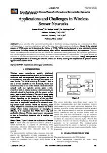
Figure 1: (a) Two-hop network architecture (ISA SP100 compliant) for deployment testing; (b) 3D-CAD model of the industrial sites for testing: flare unit (on top) and furnace structure (at bottom).

points to improve the coverage, it might be required to reopen excavations along the cable route which is totally unacceptable during the commissioning (or even before the commissioning) phase of the plant. Accurate network planning limits the need to oversize the design of the overall system, which is obviously an extra cost for the contractor. Therefore, it is crucial to develop consistent design guidelines and tools that can guarantee a reasonable accuracy in the prediction of the wireless coverage. Making use of the 3D model of the deploying area (if available) during the design phase is also of utmost importance to achieve this result. An example of a 3D view of two oil refinery sites is illustrated in Figure 1: the wireless end devices (EDs), also referred to as sensors, can be connected by star or mesh mode towards a Gateway device, with the help of intermediate Repeater nodes serving as decode and forward relays. The Gateway device is collecting data and rerouting to a wired network. Network planning is based on the prediction of the pairwise wireless link qualities among all the devices in the distributed network: the link quality is expressed in terms of the strength of the received signal. The prediction can be supported by independent radio measurement campaigns over typical refinery environments and/or by models based on propagation theory and statistical or ray-tracing tools. Conventional empirical channel models [7] cannot fully capture the unique propagation characteristics of the industrial environments; in addition, the ray-tracing-based models [8] turn out to be not practical to process the high number of structures observed in large industrial sites [9]. This motivates the development of accurate site-specific channel models based on a small fraction of measurements taken in the refinery area. This paper addresses a novel channel model based on the diffraction theory to assess the link quality in radio environments affected by highly dense metallic building blockage.

The wireless links are partitioned into mutually exclusive classes: for each class, a separate channel model is proposed to predict the quality of the radio link. The link classification is based on the analysis of the characteristics of the obstructions that impair the wireless propagation. The 3D-CAD model of the refinery site (see Figure 1(b)) is used to identify the structure of the building blockage. Based on link classification, an optimization tool is developed for the prediction of the radio coverage and for wireless connectivity optimization. Although the channel modeling and the classification methodologies proposed in this paper are fairly general and applicable in different scenarios, the model is validated by experimental measurements using industry standard ISA SP100.11a compliant [10] devices operating at 2.4 GHz based on the IEEE 802.15.4-2011 physical layer. The measurement campaigns have been carried out in two sites located in a large-size oil refinery plant. Different practical deployment cases for coverage testing are discussed in environments characterized by blockage due to a high-density of metallic structures. 1.1. Wireless Industrial Networks: Applications and Technologies. A typical industrial environment shows relevant similarities with dense urban microcellular sites characterized by a harsh environment for short-range (10–50 m) radiofrequency propagation with metallic structures [6], changing environmental conditions, nonline of sight (NLOS), and possible colocated wireless applications running over unlicensed spectrum [11]. Industrial networks typically require low-jitter sampling period for monitoring, high-integrity data delivery of critical messages, automatic reconfiguration, and usage of redundancy in case of communication failures. The most representative application cases for wireless technology [12] are commissioning, open-loop maintenance monitoring, closedloop supervisory, and regulatory remote control. Notice that

International Journal of Distributed Sensor Networks regulatory control is characterized by stricter reliability and delay requirements compared to supervisory control (some relevant application cases are primary flow and pressure control). The commercial wireless systems predominantly use the so-called ISM bands at 2.4 GHz. Early experiments for cable replacing in regulatory control applications revealed that the traditional single-hop carrier sense multiple access (CSMA) schemes supported by WiFi (IEEE 802.11) perform poorly when adopted in a factory environment [13]. More recently, wireless extensions to PROFIBUS protocol for critical control have been analyzed by real-time simulations [14]. Today, commercial battery-operated systems are based on the IEEE 802.15.4 standard and enable data to be transmitted at a typical rate of 250 kbit/s, with up to a maximum of 10 dBm output RF power to meet the RF regulations for hazardous environments. The IEEE 802.15.4 physical layer also constitutes the basis for the WirelessHART [15] and ISA100.11a [10] industry standard protocols.

2. Wireless Standards for Industrial Monitoring and Control Low-power wireless architectures and standards widely adopted in industrial automation are reviewed in this section. This introduction is instrumental to the definition of a design tool for coverage prediction and connectivity optimization. Industrial organizations such as HART and the International Society of Automation (ISA) are currently pushing towards the definition of common specifications for wireless industrial monitoring and process automation based on the IEEE 802.15.4 standard. Below we summarize the characteristics of the most relevant network solutions. WirelessHART has been ratified by the HART Communication Foundation in 2007 as the first open wireless communication standard designed for process control applications and monitoring. Although WirelessHART adopts the IEEE 802.15.4 standard for the physical layer, the MAC layer is slightly modified as it is based on TDMA (while contention access is not allowed [15]) with guaranteed time slots assigned to the network devices. Frequency hopping spread spectrum access (FHSS) is used as proven technology to provide further improvements in terms of link gain compared to direct sequence spread spectrum (DSSS) option. The adoption of TDMA technology with precisely network-wide time synchronization is the key technology that makes WirelessHART different from other industry standards. Time synchronization is based on the Time Synchronized Mesh Protocol (TSMP). This method allows to synchronize transmitting and receiving node pairs by periodically correcting the relative time offsets misalignments. The offsets corrections are typically transmitted using standard ACK reply messages (with limited extra power consumption). The synchronous TDMA MAC sublayer is built upon the IEEE 802.15.4 physical layer for mesh network communication and defines superframes of 1 sec, fixed timeslot of 10 ms, channel hopping scheme supporting flexible blacklisting options and industrystandard AES-128 block ciphers with related keys.

3 ISA SP100.11a standard for wireless industrial automation is meant to provide the specifications for reliable and secure wireless operations for monitoring, alerting, open/closedloop quality control, and predictive monitoring applications [10]. The standard supports the interoperability of multiple radio technologies. The envisioned applications include wireless process control systems (with maximum latencies in the order of 1 sec). The protocol suite, system management, and security specifications are defined for low data-rate wireless connectivity based on IEEE 802.15.4 standard. Network and transport layers are based on UDP with support of IPv6based solutions (6LoWPAN). Coexistence with other wireless services based on IEEE 802.11x, and IEEE 802.16x standards is also addressed. Although the logical link layer of ISA SP100.11a standard has a similar structure compared to WirelessHART, the standard specifies configurable timeslots with variable durations from 10 ms to 12 ms on a superframe base. Configurable timeslots ease the development of advanced architectures based on duo-casting mechanisms, optimized coexistence, and flexibility. In ISA SP100, a transaction may consist of multiple timeslots; longer transactions can be used to extend the waiting time for multiple consecutive ACKs as required in multicast transmission. The ISA standard supports both slow and fast channel hopping schemes, thus allowing devices with imprecise timing settings to perform resynchronization and neighbor discovery. The wireless architecture supported by the standard ISA is adopted here as reference for deployment testing. As depicted in Figure 1(a), the network infrastructure consists of the following components. (i) The end devices (ED) are the input/output field instruments with the minimum set of functions that are necessary to join the network. The EDs take the role of reduced-function devices and typically do not provide any mechanism for relaying messages of other devices. (ii) The Repeaters are field EDs specifically configured to serve as relay nodes for other EDs by forming a twohop (or multihop) mesh network. In typical industrial settings where the real-time responsiveness of the monitoring network is a crucial issue, the number of hops is limited to 2, therefore, the Repeater devices act as ED range extenders. (iii) The Gateways act as access points (or sinks) and collect the measurements acquired by the field devices. In practical settings, the Gateways are connected by cables (or by broadband wireless technology) to a common network manager node and thus also act as a translator between the ISA standard and other wired protocols (Foundation Fieldbus, HART, etc.).

3. Channel Modeling In this section we introduce the channel model as instrumental to the proposed link classification approach. The wireless links without a clear line-of-sight (LOS) path undergo more severe received signal power attenuations than those where

4

International Journal of Distributed Sensor Networks

the line-of-sight (LOS) path is fully unobstructed. This additional attenuation is almost uncorrelated from the distance between the transmitter and the receiver [16]. The main scatterers/objects that are responsible for the received signal power attenuation are mostly confined within the first and second Fresnel zones as these can be considered to contribute to the main propagating energy in the wavefield [17]. For a wireless link where the direct path between the transmitter and the receiver has length 𝑑, the 𝑛th Fresnel zone is the region inside an ellipsoid with circular cross-section. The radius of the 𝑛th Fresnel zone at distance 𝑞 ≤ 𝑑 is 𝑟𝑛 (𝑞) = √𝑛𝜆𝑞 (𝑑 − 𝑞) 𝑑−1 ,

(1)

with 𝜆 the signal wavelength. We assume that any pair of wireless devices connected with an arbitrary link ℓ are deployed at fixed locations and distance 𝑑. The nodes are equipped with radio devices characterized by single omnidirectional antenna transceivers. As for typical scenarios, the Gateway antenna is mounted on an elevated point while flat terrain is assumed. The propagation model describes the correlation between the size of the (mostly metallic) obstructions located within the Fresnel volumes and the total received signal strength (RSS) experienced along the propagation path. The RSS 𝛾ℓ is thus the metric (in decibel scale) used to assess the quality of the radio link 𝛾ℓ |dB = 𝑔 ⏟⏟⏟⏟⏟⏟⏟⏟⏟⏟⏟⏟⏟⏟⏟⏟⏟⏟⏟⏟⏟ 0 (𝑑, 𝛼) − 𝜎 + 𝑠. 𝑔ℓ

(2)

It combines (i) a static component 𝑔ℓ characterized by a distance-dependent LOS term 𝑔0 (𝑑, 𝛼) and an excess attenuation 𝜎 that accounts for the building blockage; (ii) a zeromean random term 𝑠 accounting for the fluctuations of the received power with typical standard deviation around √E[𝑠2 ] = 3 ÷ 5 dB in static environments [6]. In what follows, it is derived a model for the static RSS component 𝑔ℓ . The model is instrumental to the prediction of the average radio link quality for connectivity optimization (see Section 5). The distance-dependent static component 𝑔0 (𝑑, 𝛼) describes the channel gain observed over the flat terrain and without obstructions. The term 𝜎 denotes the additional signal attenuation as a function of the size and the density of the metallic objects located within the Fresnel volume (i.e., blocking the LOS path). The model used to characterize the additional attenuation component 𝜎 is derived in Section 3.1. As observed in [18], the reflection of the radio signals from the flat terrain does not influence the attenuation parameter 𝜎 but only the term 𝑔0 (𝑑, 𝛼) and the path-loss exponent 𝛼. The model is validated based on measurements over the refinery sites (see Section 6). The distance-dependent loss factor 𝑔0 (𝑑, 𝛼) can be modeled as a function of the path-loss exponent 𝛼 (see [16]): 𝑔0 (𝑑, 𝛼) = 𝑔0 − 20 log10 (

1+𝑑 ) 𝑑0

1+𝑑 − 10 (𝛼 − 2) log10 ( ), 𝑑𝐹

(3)

where 𝑔0 = 𝑔0 (𝑃𝑇 ) is the channel gain function of the transmit power 𝑃𝑇 and measured at a reference distance 𝑑0 (𝑑0 = 2 m typical), while 𝑑𝐹 =

2ℎ𝑚 ℎ𝑝 𝜆

,

(4)

is the Fresnel distance being a function of the antenna heights from the ground ℎ𝑚 and ℎ𝑝 for the pair of devices (𝑚, 𝑝), respectively. Path loss exponent is typically set to 𝛼 = 2 in short-range environments [16] where ground reflections can be neglected, for 𝑑 < 𝑑𝐹 . Larger path loss exponents 𝛼 > 2 are caused by reflections from the ground and can be experimented in long-range cases for 𝑑 > 𝑑𝐹 . The probability 𝑃𝐸 of successful communication depends on the random fluctuations of the RSS as in (2). Successful communication is modeled by outage probability such that 𝑃𝐸 = Pr [𝛾ℓ ≥ 𝛽]. The threshold 𝛽 is typically set to 𝛽 = −85 dBm such that 𝑃𝐸 ≤ 10−6 [5]. Any link experiencing 𝛾ℓ < 𝛽 is assumed as unreliable, and thus, it should not be accounted for during network planning. 3.1. Diffraction Model for Prediction of Building Blockage. It is assumed that the additional attenuation 𝜎 in (2) is due to propagating wavefronts diffracting around the building blockage consisting of metallic obstacles with different dimensions. Obstacles are acting as perfectly absorbing interfaces. The diffraction model for the building blockage term 𝜎 is based on the Fresnel-Kirchhoff method [19]. The attenuation 𝜎 in (2) is obtained as a function of the received electric field 𝐸: 󵄨󵄨 𝐸 󵄨󵄨 󵄨 󵄨󵄨 𝜎 = −20 log10 󵄨󵄨󵄨 󵄨. (5) 󵄨󵄨 𝐸free 󵄨󵄨󵄨 The ratio 𝐸/𝐸free describes the obstruction loss in excess of the free space field 𝐸free . Large-size metallic objects obstructing the wireless link absorb a large amount of the signal intensity and limit the received field to a small fraction (being 𝐸/𝐸free ≪ 1) of the one that would be observed under free-space propagation (without obstructions). A simplified description of the propagation environment (with obstacles blocking the LOS path) is considered in Figure 2. To simplify the reasoning, we assume that the obstacles surrounding the transmitter and the receiver antennas lie in the far-field region. In addition, the shape of the obstacles obstructing the Fresnel zones is squared or rectangular. Shapes that are more typical in refinery sites (tubes, structural pipe racks, etc.) have been approximated by matching a number of rectangles in the (𝑥, 𝑦) plane to get the same shape of the obstructed areas; this is also illustrated in [20]. For the 𝑖th object, the clearance zone F𝑖 in the (𝑥, 𝑦) plane denotes the region corresponding to the Fresnel volume cross-section that is free from any obstacle. The shaded region R𝑖 in the same plane indicates instead the complementary portion of the surface occupied by the obstacle. The Fresnel-Kirchhoff approach is used to model the field loss 𝐸(𝑞𝑖 )/𝐸free caused by a single 𝑖th obstacle located at distance 𝑞 = 𝑞𝑖 ≤ 𝑑. The Huygens principle is used to predict


5

Diffraction model

RX

First obstacle (largest) 𝑏1

𝑏2

𝑎2 Second obstacle

𝑎1

TX ℎ𝑎

2D front view ℜ1 𝑦

𝑎1 𝑏1

ℎ𝑏

1∘ Fresnel volume

𝑑

𝑞2

𝑞1

Short range: 𝑑 < 𝑑𝐹

2D side view 𝑦 First obstacle (largest) Neglected 𝐹1 Fresnel obstacles Second zone obstacle clearance 𝑏1 ̃𝑏2 𝑏2 𝑥 𝑟1 (𝑞1 ) >0

ℎ𝑎

𝑧

ℎ𝑏 𝑞1

𝑞2

Far-field distance

Figure 2: Fresnel-Kirchhoff method for modeling the attenuation caused by objects acting as perfectly absorbing 2D interfaces. Any hidden obstacle located in the shadow area caused by larger structural blockage can be neglected as irrelevant for additional loss.

the actual field strength diffracted by one obstacle modeled as a knife edge. The 2D model takes into account both the lateral and the vertical profiles of the obstruction by integrating the exponential phase term of the spherical wavefields over the two dimensions [19]. The electric field 𝐸(𝑞𝑖 ) measured at the receiver may be interpreted as generated by a virtual array of Huygens sources located in the plane of the single obstacle 𝑖 at distance 𝑑 from the receiver. Considering an object located at distance 𝑞𝑖 from the transmitter and occupying an area (𝑥, 𝑦) ∈ R𝑖 , the field loss 𝐸(𝑞𝑖 )/𝐸free can be approximated for (𝑥, 𝑦) ≪ 𝑞𝑖 , 𝑑 − 𝑞𝑖 as [19] 󵄨󵄨 󵄨󵄨 𝐸 (𝑞 ) 󵄨󵄨 󵄨󵄨󵄨 󵄨󵄨 −𝑗𝜋 (𝑥2 +𝑦2 ) 1 󵄨󵄨 𝑖 󵄨󵄨 󵄨󵄨 󵄨 󵄨 󵄨󵄨 ] 𝑑𝑥 𝑑𝑦󵄨󵄨󵄨󵄨 , 2 󵄨󵄨 𝐸free 󵄨󵄨󵄨 ≃ 󵄨󵄨󵄨1−𝑗 ∫(𝑥,𝑦)∈R 𝑟2 (𝑞 ) exp [ 𝑟1 (𝑞𝑖 ) 󵄨󵄨 𝑖 𝑖 󵄨 󵄨󵄨 󵄨 1 󵄨 (6) where 𝑟1 (𝑞𝑖 ) defined in (1) refers to the radius of the 1st Fresnel volume circular section corresponding to the location of the obstruction. The approximation reasonably fits with the considered environment (see Section 6) as far as the obstacle is confined within the Fresnel volume. To gain further insight into the interplay between the obstruction size and the corresponding field loss, in what follows we focus on the example of a single obstacle obstructing the LOS path with rectangular cross-section described by lateral and vertical half-dimensions (𝑎𝑖 , 𝑏𝑖 ). The loss term in

(6) simplifies for the case of large obstacle |𝑎𝑖 |, |𝑏𝑖 | ≫ 𝑟1 (𝑞𝑖 ) as (see the appendix) 󵄨󵄨 𝐸 (𝑞 ) 󵄨󵄨 󵄨󵄨 √2𝑏𝑖 √2𝑎𝑖 󵄨󵄨󵄨󵄨 󵄨 󵄨󵄨 𝑖 󵄨󵄨 󵄨󵄨 ≈ 󵄨󵄨󵄨1 − 2𝑗 × Γ ( 󵄨󵄨 ) Γ ( )󵄨󵄨 󵄨󵄨 𝐸free 󵄨󵄨 󵄨󵄨 𝑟1 (𝑞𝑖 ) 𝑟1 (𝑞𝑖 ) 󵄨󵄨󵄨 󵄨 󵄨 󵄨

(7)

with 1 1 1 1 1 1 Γ (𝑥) = [ + sin ( 𝜋𝑥2 )] − 𝑗 [ − cos ( 𝜋𝑥2 )] . 2 𝜋𝑥 2 2 𝜋𝑥 2 (8) Figure 3 compares the diffraction loss for a single object obstructing the LOS path with varying square cross-sections (𝑎1 = 𝑏1 ) measured with respect to the Fresnel radius 𝑟1 (𝑞1 ). Model (6) and approximation (7) are in solid and dashed lines, respectively. The field loss caused by an object fully obstructing the 1st and the 2nd Fresnel circular section such that 𝑎1 /𝑟1 > √2 lies below 𝐸/𝐸free < 40%. The general model (6) for a single obstacle can be extended to multiple obstacles by following the Deygout approach [21]. For multiple obstacles, the lateral 𝑎𝑖 and vertical 𝑏𝑖 dimensions of the shaded region R𝑖 for the 𝑖th obstacle are calculated with respect to the size of the largest obstacle (obstacle 𝑖 = 1 in the example of Figure 2). For each dimension, the Deygout method requires to find the 𝑖th object (edge) with the largest value of parameters (𝑎, 𝑏) compared to the Fresnel size, such that 𝑎 = arg max𝑎𝑖 [𝑎𝑖 /𝑟1 (𝑞𝑖 )] and 𝑏 = arg max𝑏𝑖 [𝑏𝑖 /𝑟1 (𝑞𝑖 )] and ignoring all the other edges. Based on the selected set of obstacles, a new reference plane is created

6


80 70

𝜆) within the first and second Fresnel volume, while obstacles might instead occupy the remaining Fresnel volumes. The nominal (such that from (2) 𝐸[𝛾𝑎,𝑏 ] ≥ 𝛽) maximum range to guarantee a reliable connection is found as 𝑅 ≃ 150 m (for RSS above 𝛽 = −85 dBm). In the worst-case scenario where obstacles completely obstruct the 𝑛th Fresnel volumes with 𝑛 ≥ 3, the observed received electric field intensity from (6) is the 𝐸/𝐸free = 90% fraction of the one that would be measured in the free-space case (thus corresponding to an attenuation of 𝜎(ℓ) ≃ 1 dB [22]).

2D front view ℜ1 𝑦

) (6 el od M

𝐸(𝑞1 )/𝐸free (single obstacle %)

90

(7) on ati xim pro Ap

100

𝑎1

𝑎1

𝐹1 𝑥 𝑟1 (𝑞1 ) >0

60 50 40 30 20 0.8

1

1.2

1.4

1.6

1.8

2

2.2

Object size (𝑎1 = 𝑏1 ) : 𝑎1 /𝑟1 (𝑞1 )

Figure 3: Diffraction loss caused by an object with square crosssection (𝑎1 = 𝑏1 ) and obstructing the LOS path. Energy loss 𝐸/𝐸free is analyzed with respect to the ratio 𝑎1 /𝑟1 (𝑞1 ).

for each dimension and used to compute the contributions of all the intermediate edges with modified size, 𝑎𝑖 = 𝑎̃𝑖 , 𝑏𝑖 = ̃𝑏𝑖 (see Figure 2). The overall obstruction loss 𝐸/𝐸free for 𝐵 > 1 obstacles with meaningful obstructing size at distance 𝑞𝑖 is obtained by multiplying each contribution along the LOS path so that [21] 󵄨 𝐵 󵄨󵄨 󵄨󵄨 𝐸 󵄨󵄨 󵄨 𝐸 (𝑞𝑖 ) 󵄨󵄨󵄨 󵄨󵄨 󵄨󵄨 󵄨󵄨 , 󵄨󵄨 = ∏ 󵄨󵄨󵄨󵄨 󵄨󵄨 󵄨󵄨 𝐸free 󵄨󵄨 𝑖=1 󵄨󵄨 𝐸free 󵄨󵄨󵄨

(9)

where each term 𝐸(𝑞𝑖 )/𝐸free is in (6) or approximated as in (7). In spite of the simplicity of this method, in Section 6, it is proved to be accurate enough for wireless link quality prediction.

4. Wireless Link Classification The proposed approach for the evaluation of the pairwise link channel qualities is validated by a database of radio measurements taken in different refinery sites to cover the most representative scenarios. Based on the experimental measurements, 5 mutually exclusive link categories have been defined to account for the different sizes and the positions of the most typical obstructions inside the (1st and 2nd) Fresnel volumes surrounding the considered links. The analysis of the building blockage property is based on the inspection of the full 2D/3D model of the plant. Each link type is characterized by a specific configuration of the Fresnel zone clearance that corresponds to a reference value for the obstruction loss 𝐸/𝐸free according to the model outlined in Section 3. For each link type ℓ, the loss 𝜎 = 𝜎(ℓ) is computed as in (5), and it is used to predict the average link quality 𝑔ℓ in (2). Based on the experimental activity, five different linktypes are considered (see Figure 4). Type I. LOS (ℓ = 1) link type is characterized by the absence of obstacles (with dimensions larger than the signal wavelength

Type II. Near-LOS (ℓ = 2) link type is observed in environments where the obstacles are located in the first Fresnel outer region at distance 0.6 × 𝑟1 (𝑞) from the direct path. The shaded subregion in Figure 4 can be considered as a “forbidden” region: if this region is kept clear, then the total path attenuation will be practically the same as for the unobstructed case (Type I). This clearance zone is thus used here as a criterion to decide whether an object is to be treated as a relevant obstruction. The radio propagation for this link category is characterized by an additional signal energy loss compared to Type I. Based on the radio measurement campaigns and the diffraction model in (6), the Type II links typically retain the 𝐸/𝐸free = 70% of the electric field observed in the free-space case (𝜎(ℓ) ≃ 3 dB). The theoretical maximum range reduces to 𝑅 ≃ 108 m. Type III. Obstructed-LOS (ℓ = 3) link type is observed in environments where the obstacles are located inside the forbidden region, although the direct path connecting the transmitter and the receiver is still unobstructed. The links belonging to this category retain approximately 𝐸/𝐸free = 40% of the electric field that would be measured in the freespace case. The theoretical maximum range is 𝑅 ≃ 60 m. Type IV. NLOS (ℓ = 4) link type is characterized by large objects obstructing the direct path between transmitter and receiver; therefore, 𝐸/𝐸free < 40% (𝜎(ℓ) ≃ 8 dB): the size of those objects is such that a clearance zone is still visible, ⋂𝑖 F𝑖 ≠ 0, suggesting that there might be the possibility of reliable communication. Being the forbidden region and the LOS path both obstructed, the reference value for the field loss is chosen as 𝐸/𝐸free = 20% (𝜎(ℓ) ≃ 14 dB). The theoretical maximum range further reduces to 𝑅 ≃ 32 m. Type IV-S. Severe-NLOS (ℓ = 5) link type refers to a severe NLOS environment where the first and the second Fresnel regions are completely obstructed by one or more obstacles with significant size (and dimensions scaling as ∼ 4 ÷ 5𝑟1 (𝑞)), so that the observed received electric field falls below 𝐸/𝐸free = 10% compared to the one that would be measured in the free-space case (𝜎(ℓ) ≃ 21 dB). The theoretical maximum range is 𝑅 ≃ 15 m. This model type resembles a propagation environment where the line-of-sight path is blocked by large-size concrete buildings [18].

5. Radio Planning Optimization The wireless network deployment problem refers to the determination of the positions of the wireless nodes such that


7 Type II: near LOS

Type I: LOS 𝑟1 (𝑞) TX

RX

0.6 𝑟1 (𝑞1 )

TX

𝑞

RX 𝑞

𝐸/𝐸free ≥ 90%

𝑑

𝑑

𝐸/𝐸free = 70%

First Fresnel region

Unobstructed region

Type III: obstructed LOS 𝑟1 (𝑞) = √𝜆𝑑−1 𝑞(𝑑 − 𝑞)

0.6 𝑟1 (𝑞1 )

First Fresnel region

RX 𝑞 𝐸/𝐸free = 40%

𝑟2 (𝑞) = √2𝜆𝑑−1 𝑞(𝑑 − 𝑞) Second Fresnel region

𝑑 Direct path free from obstacles Type IV: NLOS

Type IV-S: severe NLOS 𝑟2 (𝑞)

𝑟2 (𝑞)

𝑟1 (𝑞)

𝑟1 (𝑞)

TX

RX

TX 𝑞

𝑞 𝑑 𝐸/𝐸free = 20%

≅4𝑟1 (𝑞)

TX

RX

𝑑 𝐸/𝐸free ≤ 10%

Figure 4: Proposed link classification and Fresnel clearance zones.

some limiting values of coverage, connectivity, and energy efficiency can be achieved [23]. Wireless device deployment strategies for coverage and connectivity enhancement play a crucial role in providing better quality of service (QoS) to the network. The coverage and the connectivity problems are two fundamental issues that have been widely studied in the literature [24]. In coverage problems, the objective is to deploy wireless sensor devices in strategic ways such that an optimal area coverage is achieved given the requirements of the underlying application [23]. The coverage problem therefore deals with placing a minimum number of nodes so that every measurement point in the sensing field is optimally covered according to applicationspecific constraints. In industrial monitoring and control applications, the position of the measurement points (sensors or actuators) is constrained by the application; therefore, the coverage optimization is typically carried out based on the structure of the process unit. The focus of this section is thus on connectivity optimization, as this is the most crucial problem for cable replacing in the industrial networking context. In what follows, we first report on the current state of the research on optimized node placement in wireless sensor networks (Section 5.1). Next, we discuss relevant practical issues

and rules that are specifically tailored for network and connectivity optimization in industrial networks (Section 5.2). Finally, we propose an optimization framework tailored for commercially available ISA SP100 two-hop networks that allows the optimal selection of the devices that need to be configured as Repeaters (Section 5.3). The goal is to optimize the number and the position of the infrastructure devices (e.g., the Repeater nodes and/or the Gateways) to guarantee a reliable connection between the measurement points and the control unit with some degree of redundancy [25]. Optimally deployed wireless infrastructure devices guarantee adequate QoS (i.e., outage probability), long network lifetime, and thus reduced costs for network maintenance. The proposed deployment problem is based on the prediction of the RSS for all the pairwise wireless links according to channel modeling and classification outlined in Sections 3 and 4. 5.1. Node Deployment Strategies in Wireless Sensor Networks: A Survey. Extensive work has been reported in the literature relating to wireless sensor and relay node deployment. Deployment of nodes has been considered for targeting connectivity, coverage, node lifetime, and/or QoS. The deployment strategies can be classified into static and dynamic [26] depending on whether the optimization is performed

8 during network setup or during network operation (for node repositioning, see [26]). In static environments where data is periodically collected over preset routes, the problem of optimal node placement for connectivity maximization has been proven to be NP-hard for most of the formulations [27]. Several heuristics and rules have been therefore proposed to find suboptimal solutions based on graph theory. Several approaches to the problem of placing nodes are addressed in [24] to achieve 𝐾-connectivity at the network setup time so that 𝐾 independent paths are identified for every pair of devices. The majority of published work on sensor network deployment limits its focus on simplified and analytically tractable 1D and 2D environments where connectivity can be considered as a primary/secondary objective or as a constraint in the deployment problem [26]. For example, in [28] an outdoor random deployment which targets the connectivity as a primary objective in 2D space is investigated. In [29], a constrained multivariable nonlinear programming problem is analyzed to determine the locations of the sensor nodes to maximize the network lifetime, given a fixed number of sensor nodes with certain coverage and connectivity requirements. A deployment strategy for sensor networks is introduced in [30] to balance the network lifetime and connectivity goals for single- and two-hop networks. Focusing on large-scale sensor network applications, controlled placement of nodes is often focused on a subset of network devices (e.g., Repeaters or relays) with the goal of designing the network topology to achieve the desired application requirements [31]. The problem of relay placement in two-hop networks is analyzed in [32]: the objective is to place the fewest number of relay nodes so that each sensor node can communicate with at least one relay node, and the network of relay nodes is connected. The goal is to guarantee a reliable communication between each pairs of sensor nodes while the same reasoning can be extended for sensors communicating with a common Gateway node. Recent literature considers the problem of connectivity in massively dense sensor networks [33]. The problem of deploying relay nodes in heterogeneous sensor network scenarios is considered in [34] where sensor and relay nodes possess different transmission ranges (e.g., through the use of different hardware, antennas, or high-power radio modules). The work [35] considers a scenario where sensor devices are equipped with directional antennas: the goal is to find an optimal subset of locations to minimize the total network cost while satisfying the requirements of coverage and connectivity. The network connectivity problem is mostly considered for 2D planning with the assumption of simple binary communication disk model without looking at site-specific environmental constraints (see also [34–37]). Those approaches are very prone to failure in practical large-scale industrial applications. Some attempts in the literature have been made towards the analysis of deployment and connectivity problems in 3D environments, although the topic is still considered an open issue [38]. The problem of modeling and connectivity optimization in random 3D networks has been recently addressed in [38, 39] where the deployment problem considers the maximization of network connectivity satisfying lifetime constraints.

International Journal of Distributed Sensor Networks 5.2. Connectivity Optimization in Wireless Industrial Networks. The connectivity optimization for industrial networks can be in general applied to two-hop large-scale networks consisting of Gateways, relays, and sensors, operating in time (and safety) critical applications [36, 37]. Three general practical rules [40] should be followed during system design and configuration. These are summarized below. Gateway Deployment Planning. The wireless network is first divided from a single process unit into subsections (subnetworks). Within each subsection, the position of the measurement points, and thus the degree of coverage, is designed to satisfy application-dependent requirements. The devices (or end devices, EDs) are deployed to collect data from the nearby measurement points (depending on the monitored process, EDs might consists of a single or multiple measurement points). Each process unit subsection is served by one Gateway (acting as access point for the corresponding devices). The Gateway should be able to allocate resources for two-way communication in real time with the EDs. For smallsize projects (as those analyzed in Section 6), a single Gateway is sufficient if the total number of measurement points is less than the capacity 𝐶 of the Gateway point. Instead, if the project is large with several hundreds of wireless devices and process units, a single network manager should manage multiple Gateways. The required number of Gateways can be defined as a function of the number of measurement points. The following simple calculation can be used in practice to approximate the number of Gateways 𝐺 needed: −1

𝐺 = 𝑁 × [𝐶 × (1 − 𝜌sc )] ,

(10)

where 𝜌sc is the spare (or residual) fraction of the available capacity 𝐶 to be reserved for emergency signalling with capacity measured in terms of number of measurement points served. 𝑁 is the number of measurement devices assuming that each ED is serving as a single measurement point. A typical design rule prescribes that 𝜌sc = 40% [40]. The Gateway capacity 𝐶 depends on the wired/wireless protocol used for data transfer towards the network manager. Connectivity Optimization. The use of site-specific radio propagation models (empirical or ray-tracing based) enables the optimization of the connectivity for virtual network planning. A propagation model can be therefore exploited as instrumental to the prediction of the RSS, from which the quality of the radio link (and of the end-to-end connectivity) can be inferred with some degree of accuracy. Prediction errors are typically caused by modeling mismatches (e.g., link classification errors) or unpredictable RSS fluctuations (see Section 3) due to interference over the 2.4 GHz band or fading induced by objects or people moving in the area. The solution to the connectivity and the Gateway deployment problems is generally well understood in the literature (see, e.g., [41]). In the industrial context, three practical rules are defined to ensure a sufficiently high link reliability. The rules are summarized as follows (see also [40]). (i) Rule 1. Every network with more than 5 devices should have a minimum of 25% of devices within

International Journal of Distributed Sensor Networks the effective range of the Gateway to ensure mesh connection (typically over a maximum number of 3÷ 4 hops). In any case, every network should have a minimum of 5 infrastructure devices within the effective range of the Gateway. Example: a network consisting of 100 EDs requires 25 EDs at minimum within the effective range of the Gateway (directly connected). (ii) Rule 2. Gateway RF antenna should be mounted at least 2 m from the ground level and should not be surrounded by obstacles. Obstacles should lie at distance 2𝜆 from the antenna. (iii) Rule 3. Every device should have a minimum of 3 neighbors in the effective range. This ensures that when implemented, there will be at least one reliable routing path to the Gateway alternative to direct connection (to guarantee 𝐾 = 2 connectivity). On-Site Stress Testing. Stress testing of the deployment design is recommended during an on-site survey to verify potential weaknesses highlighted during the virtual network configuration. Stress testing is performed by altering the position of the EDs from the nominal position and thus by measuring the fluctuations of the RSS field. Although the context may vary slightly depending on the structure of the environment, almost all these basic steps could be applied regardless of the specific commercial system and standard (i.e., WirelessHART or ISA SP100, see Section 2). The first and the second steps are known to be the most critical for high density applications [12]. 5.3. Optimal Repeater Configuration for Two-Hop ISA Industrial Networks. The wireless network for industrial environment under consideration conforms with the standard ISA SP100.11a and is characterized by one Gateway collecting data from wireless end devices (EDs). A subset of EDs might serve as Repeater nodes acting as range extenders. The Gateway node is an electrically powered device, serving as access point for the EDs. It manages both wireless and wired interfaces. The Repeaters are configured as EDs with superior functionalities: these allow to connect to the Gateway and simultaneously serve as decode and forward relays for extending the range of the neighboring EDs. Repeater nodes are more expensive than standard EDs since they must be preconfigured to multiplex different sensor data and could be more powerful in terms of processing and transmission capabilities. The connectivity optimization problem is therefore focused on the Repeater configuration. The candidate sites for the deployment of the EDs and of the Gateway node are assumed to be assigned: each candidate site might host either a Repeater node multiplexing sensor data or a standard ED without relaying functionalities. Optimal placement of the Gateway is not addressed in this paper, although we only assume that Gateway locations satisfy connectivity Rule 2 (see Section 5.2). Optimal deployment for the Gateway might be carried out as illustrated in [41], even if, in practical

9 industrial scenarios, the exact position is subject to stringent environmental constraints. The optimization approach is based on the selection of the smallest subset of devices that need to be configured as Repeaters to guarantee network connectivity. The optimization jointly minimizes the number of EDs connected to the corresponding Gateway over two hops [32] and guarantees a minimum quality of service for all links, so that the static RSS component 𝑔ℓ is kept for all the configured links above the system threshold 𝛽 (see Section 3) herein adopted as the minimum tolerable link quality. The static RSS component is predicted based on the 3D model of the plant, as done in Section 3. Let the wireless network be represented by a set S of 𝑁 nodes located at known positions within a specific area of the plant. A sequence of messages is continuously transmitted by the EDs towards a common Gateway node labeled as “0” possibly with the help of one intermediate node serving as a Repeater. To comply with the real-time responsiveness constraints typically required by industrial closed-loop control applications, the maximum number of hops to reach the Gateway node is herein limited to 2: the same constraint is also adopted in recent ISA compliant network implementations. Any wireless node 𝑎 ∈ S is said to be connected with reasonable quality to the Gateway node “0” if and only if 𝑖𝑎,0 = 1 where the indicator 𝑖𝑎,0 for an arbitrary link ℓ := (𝑎, 0) is defined as 𝑖𝑎,0 = 1 iff 𝑔ℓ > 𝛽,

𝑖𝑎,0 = 0 otherwise,

(11)

while sensitivity threshold 𝛽 accounts for the random fluctuations of the static RSS component 𝑔ℓ . Deployment optimization consists of three phases. Selection of Candidate Repeaters. First, it is defined the subset S0 ⊂ S of 𝑁0 nodes without direct connection to the Gateway S0 := {𝑎 ∈ S | 𝑖𝑎,0 = 0 ∀𝑎} .

(12)

The same nodes 𝑎 ∈ S0 are preconfigured as EDs, and they should not provide relaying functionalities. The remaining subset S1 := S \ S0 S1 := {𝑎 ∈ S | 𝑖𝑎,0 = 1 ∀𝑎} ,

(13)

of 𝑁1 = 𝑁 − 𝑁0 devices observing a reliable connection with the Gateway can be assigned either as Repeaters or EDs. The optimal configuration of devices in subset S1 is carried out in the following steps. Feasibility Region for the Connectivity Problem. Assuming all nodes 𝑏 ∈ S1 be initially configured as Repeaters, a solution to the connectivity problem satisfying Rule 3 for the EDs 𝑎 ∈ S0 without a reliable direct connection with the Gateway exists if ∑ 𝑖𝑎,𝑏 > 0,

𝑏∈S1

∀𝑎 ∈ S0 ,

(14)

such that all the EDs 𝑎 ∈ S0 can exploit an alternative twohop link through one Repeater 𝑏 ∈ S1 serving as a range

10


extender. In case the condition is not satisfied, the number of candidate points is not sufficient for a feasible solution to the coverage problem; additional candidate sites must be therefore identified. New candidate sites must be assigned during the precommissioning of the plant; the deployment should thus account for application and site-specific environmental constraints. 𝑁

1 ( 𝑁𝑛1 ) potential Repeater Configuration. Among the 𝐾 = ∑𝑛=1 subsets R𝑘 ⊆ S1 of devices configured as Repeaters, with 𝑘 = 1, . . . , 𝐾, the optimal subset is defined as the one satisfying the feasibility region (14) and with the smallest cardinality. By letting |R𝑘 | be the cardinality of the 𝑘th subset R𝑘 , the algorithm identifies the optimal 𝑘th subset of the Repeater devices R𝑘 ⊆ S1 such that

󵄨 󵄨 R𝑘 := arg min 󵄨󵄨󵄨R𝑘 󵄨󵄨󵄨 𝑘

s.t.

∑ 𝑏∈R𝑘 ⊆S1

𝑖𝑎,𝑏 > 0,

∀𝑎 ∈ S0 .

(15)

The devices 𝑏 ∈ R𝑘 are thus configured as Repeaters while the other devices 𝑎 ∈ S \ R𝑘 take the role of EDs. Notice that S0 ⊆ S \ R𝑘 . The iterative algorithm described as follows is used to find a solution to problem (15). Let the ordering of the Repeater subsets be such that ∀𝑘 |R𝑘 | ≥ |R𝑘+1 |; the algorithm starts by picking the largest feasible set of Repeaters, so that R1 ≡ S1 and iteratively identifies new feasible subsets R𝑘 ⊂ S1 with smaller cardinality (𝑘 > 1) by randomly removing nodes from S1 . The optimal subset R𝑘 solution to (15) is such that any smaller subset of Repeaters Rℎ with ℎ > 𝑘 is not feasible as ∏ ∑ 𝑖𝑎,𝑏 = 0,

𝑎∈S0 𝑏∈Rℎ

∀ℎ > 𝑘,

(16)

or, equivalently, for any Repeater subset Rℎ with smaller cardinality Rℎ ⊂ R𝑘 the sum ∑𝑏∈Rℎ 𝑖𝑎,𝑏 = 0 for some ED 𝑎 ∈ S0 without reliable direct connection.

6. Experimental Activity The experimental validation of network connectivity is based on the link classification and channel modeling described in Sections 3 and 4. The optimization tool used for the optimal selection of the Repeater nodes is described in Section 5. The connectivity design consists of three steps. At first, the candidate positions for the wireless devices are chosen to highlight practical cases of meaningful interest for the deployment of an industrial network. The Gateway node is mounted above ground (according to Rule 2 in Section 5.2) and collects the data received from all the EDs. Second, the pairwise link RSSs are predicted based on channel modeling and classification as outlined in Sections 3 and 4. Finally, the optimal sub-set of the wireless devices that should act as Repeaters is computed based on the connectivity optimization tool illustrated in Section 5.3.

In the proposed experimental set-up, we deployed absolute and gauge pressure transmitters communicating with a Gateway node by star or two-hop mesh topology. Compared to mesh topology, deploying a star topology network should be preferred in practice as it provides better performance in terms of per-link real-time responsiveness that is required for monitoring and control of critical plant parameters. The radio transceivers conform with the ISA SP100.11a protocol [10] with radio transmit power set to 𝑃𝑇 = 11.6 dBm. The experiments have been carried out in two sites within the same oil refinery: the first site is a 100 m × 200 m area around a flare unit; the second one is a 60 m × 30 m area surrounding a furnace structure. All the environments under consideration are characterized by metallic objects and concrete buildings with high-reflectivity surfaces. Before the test, we used a signal analyzer to characterize the interferers in the area. Since no significant activity was detected, the IEEE 802.15.4 channels selected for the experiments have center frequencies 2.405 GHz and 2.480 GHz, corresponding to the ISA SP100.11a channel numbers 1 and 15, respectively. The static RSS component 𝑔ℓ in (2) characterizing the radio propagation over each link is predicted by following three steps. (i) Step 1. The number and size of the objects blocking the direct path between the transmitter and receiver pair (or the corresponding Fresnel volumes) are identified by analyzing the 3D model of the plant. (ii) Step 2. The link is classified by exploring the 3D maps of the corresponding sites. Based on the link types identified in Section 4, the size of the obstructions is compared with the Fresnel volumes to identify the corresponding clearance zones F𝑖 for the obstacles with relevant size compared to the wavelength 𝜆. The link category is then selected by comparing the resulting clearance zones with the ones characterizing each link type. (iii) Step 3. The static RSS component 𝑔ℓ is predicted according to the chosen link type. The signal attenuation 𝜎 = 𝜎(ℓ) in (2) for the chosen link category ℓ is computed based on the predicted field loss 𝐸/𝐸free as in (5). The distance-dependent loss factor 𝑔0 (𝑑, 𝛼) is defined according to the position of the transmitter and receiver devices. In all of the considered short range cases for 𝑑 < 𝑑𝐹 , the path loss exponent is 𝛼 = 2. The propagation over long ranges such that 𝑑 > 𝑑𝐹 suffers from a larger path loss due to ground reflections: for a typical case of 𝑑𝐹 ≃ 50 m (Gateway at 6 m from the ground), the available measurements indicate a path loss exponent of 𝛼 = 2.5. The measurements analyzed in the following sections highlight the accuracy of the proposed channel characterization and modeling approach. Tightness of the proposed model is verified by comparing the predicted RSSs with the corresponding measurements obtained during the on-line testing. The model accuracy is found as reasonably high in all the considered settings (with errors below 4 dB for all the considered cases).


11

Deployment case number 1

Deployment case number 2 B1a + B1b B2b + B2c C1b

B2a

B1c

C1a

C1c

Unreliable connection D1a

D1b C2a + C2b

(a)

+ C2c (b, c)

D2a + D2b + D2c Deployment case number 3

Unreliable connection

Deployment case number 4 B4a

B3a + B3b

C4a

D4a Unreliable connection

D3a

C3a + C3b C3c (Repeater) Unreliable connection Flare unit top view

Type I Type II Type III

6m

Type IV Type IV-S

Figure 5: Flare unit test sites and link classification according to the categories defined in Section 4. Links are colored based on the selected link type; unreliable links are also highlighted.

6.1. Site Test No. 1: Flare Unit. In this test, the Gateway is mounted in 4 different locations corresponding to different deployment cases as illustrated in the floor plan maps of Figure 5. For deployment case no. 1 the height from the ground of the Gateway is 1.5 m (𝑑𝐹 ≃ 25 m); for the remaining cases; the height is above 6 m (𝑑𝐹 ≃ 50 m). For all cases, the 3 EDs labelled as B, C, and D are acting as input/output field devices and are moved in different positions labeled by lowercase letters (𝑎, 𝑏, and 𝑐). The corresponding RSS measurements are reported by circle markers for all the deployment cases and analyzed in Figure 6 for devices at ground level and in Figure 7 for devices at 1 m above ground.

The markers have different colors to identify the link category while the link classification is based on the inspection of 2D and 3D-CAD maps. The predicted static RSS component 𝑔ℓ is represented by solid lines as a function of the distance 𝑑 and for each link category (see Section 4). The same color code used for the measurements is adopted to highlight the prediction and link classification accuracy. The effectiveness of the proposed channel characterization and modeling approach can be appreciated in several settings as highlighted in Figure 8. To focus on a relevant example, in the deployment case 3, the ED transmitters located at positions C3a (ground level) and C3b (1 m height

12

International Journal of Distributed Sensor Networks Deployment cases 1–4. Devices B, C, D (devices at ground level) −60 −65 B1a C1a

−70

(Typ. I LOS) (Typ. II nearLO S)

RSS (dBm)

B1c C4a

−75

C1c C2a

−80 −85

C1b

C2b

𝛽

(Typ.

IV N

B2a

LOS) (Typ. IV -S

No reliable connection

−90 10

(Typ. II I OLOS )

B3a

D3a

15

C3a

20

25

severe

B2b

NLOS)

30

35

38

Distance (m) Measurements Predicted model for each link cateogry

Figure 6: RSS measurements (circle markers) for devices B, C, and D over the flare unit sites (1–4) at ground level. Positions of devices are indicated by lowercase letters and correspond to the maps in Figure 5. Colors identify the link types; the predicted model for each link category is superimposed by solid lines, using the same color code.

−60

Deployment cases 1–4. Devices B, C, D (above ground > 1 m) D1b B1b

−65

(Typ. I LOS) (Typ. II nearLO S)

RSS (dBm)

−70 B3b

−75 C2a

−80 −85

C2c

𝛽

IV N

LOS)

C3c (Typ. IV-S s evere C3b NLOS )


−90 10

(Typ.

D1a

15

20

25 Distance (m)

D4a C1c (Typ. II I OLOS ) B2c

D2c D2a B4a D2b

30

35

38

Measurements Predicted model for each link cateogry

Figure 7: RSS measurements (circle markers) for devices B, C, and D over the flare unit sites (1–4) located at 1 m above ground. Positions of devices are indicated using lowercase letters and correspond to the maps in Figure 5. Colors identify the link types; predicted model is illustrated using the same color code.

from the ground) are hidden behind a big cylindrical vessel that completely obstruct the 1st Fresnel region. The wireless links connected to the Gateway retain the 𝐸/𝐸free = 13% and the 𝐸/𝐸free = 9% of the received field that would be measured in free space, respectively. Therefore, they can be reasonably classified as Type IV-S. As confirmed by measurements, the predicted RSS is below the critical 𝛽 = −85 dBm reliability threshold (distance 𝑑 = 26 m) suggesting the need for a Repeater device acting as relay. The same transmitter is now

moved at position C3c to circumvent the large obstruction and create more favorable propagation conditions. In this case, by analyzing the corresponding 3D map, the 1st Fresnel region is slightly unobstructed: the link retains a larger fraction (𝐸/𝐸free = 17%) of the received electric field and thus can be reasonably classified as Type IV. As confirmed by the chosen model, the connection with the Gateway is now reliable as RSS −82 dBm: this suggests to deploy a Repeater device at position C3c multiplexing the source data received from the devices obstructed by the cylindrical vessel at position C3a and C3b. As confirmed by analysis of the 3D model, the links connecting the Repeater with devices located at the other side of the vessel can be classified as Type II, being the forbidden region free from obstacles. Figure 8 highlights other relevant deployment cases: the links connecting the Gateway with the EDs at position B4a and C4a are classified as Type IV (𝐸/𝐸free = 20%) and Type III (𝐸/𝐸free = 32%), respectively. For both links the forbidden region is found as partially obstructed: in addition, at position B4a, the LOS path is blocked by concrete and metallic structures located around the corresponding ED location. For position D4a instead, the forbidden region is found as unobstructed; the corresponding link can be thus classified as Type II (𝐸/𝐸free = 63%). 6.2. Site Test No. 2: Furnace Structure. In this test, the Gateway is mounted on the stairway in the south-east of the furnace at 10 m above the ground level. In this scenario, devices C and D are moved over four different floors of the furnace structure according to Figure 9. Device B instead is located at ground level, moved in 5 positions in front of the furnace structure. The distance between each device and the Gateway ranges between 14 m and 57 m and is lower than the Fresnel distance 𝑑𝐹 ≃ 80 m in all cases. Measurements and predicted model for each link category are reported in Figure 10 using the same color code adopted for the flare unit scenario. By exploring the 2D and the 3D maps of the site, the links corresponding to positions B5 (𝑑 and 𝑒), D5e, and C5a can be reasonably classified as Type III (𝐸/𝐸free = 40% or 𝜎(ℓ = 3) ≃ 8 dB), being the forbidden region (see Figure 4) partially obstructed. Measured attenuations are 𝜎 = 5 ÷ 10 dB and confirm this choice. As highlighted in Figure 11, the NLOS links (Type IV) correspond to positions B5c, D5a, and C5e with observed attenuation ranging from 𝜎 = 11 ÷ 17 dB. For positions D5d (4rd floor) and C5d (3rd floor), the metallic structure produces a waveguide effect on propagation such that reliable communication occurs even across the whole furnace structure. The wireless signals propagate all around the furnace environment without obstacles and take advantage of the constructive interference. The positions D5b (2rd floor) and C5b (1rd floor) are instead surrounded by the furnace building that fully obstructs the 1st Fresnel volume and absorbs approximately the 84% and the 88% of the freespace field intensity, with 𝐸/𝐸free = 16% and 𝐸/𝐸free = 12%, respectively (Type IV-S). As confirmed by measurements, the predicted RSS for Type IV-S link (with distance 𝑑 = 57 m) is below the critical 𝛽 = −85 dBm reliability threshold. The installation of one Repeater device located in the example at position C5a is therefore the optimal choice to relay the data

International Journal of Distributed Sensor Networks Type IV

13 Type IV-S

C3a + C3b

C3c Cylindrical vessel blocking the 1∘ and 2∘ Fresnel volumes

e bl lia re Un lin

Obstruction traversing the LOS path

k

C3a + C3b Repeater C3c Type IV

Type IV-S

C2a + C2c (+1 m) C2a + C2b + C2c

Type II

C2b (ground)

Type III

Obstructed forbidden region (free LOS)

B4a (+1 m) Obstructed forbidden region and LOS path

C4a (ground)

D4a (+1 m) Unobstructed forbidden region

Figure 8: Flare unit scenario: relevant deployment example cases.

acquired by the measurement points located at positions D5b and C5b. 6.3. Long-Range Testing. Although the focus of this paper is mostly on short-range networking modeling and optimization of network deployment in industrial environments, a long-range test have been also carried out as depicted in Figure 12 (deployment case 5) with the Gateway located in

the same position of case 4 while the device C at ground level has been moved in two sites. The first one is an open area classified as near LOS environment (Type II) on the right side of the flare unit at distance 109 m from the Gateway, the second site was located at distance 132 m from the Gateway in the southern part of the flare unit where the LOS path is obstructed by a building. The path loss 𝑔0 caused by the ground reflections (flat terrain) can be reasonably modeled

14


Furnace structure

B5b

C5b + D5b

Map view

C5a + D5a

B5a

C5e + D5e

B5d B5c B5e

4∘ floor 3∘ floor 2∘ floor 1∘ floor

D5d C5d D5b C5b

ℎ = 10 m

3m

Front view devices C, D

D5c, D5e C5c, C5e D5a C5a

18 m

10 m

C5c + D5c

C5d + D5d

2m

(a)

D5b (2∘ floor) NLOS

D5d (4∘ floor)

3D view devices C, D

C5a (1∘ floor) NLOS

C5d (3∘ floor) e uid eg t av W effec

Air duct

D5a (2∘ floor) NLOS

D5e (4∘ floor)

D5c (4∘ floor) C5c (3∘ floor)

C5a (1∘ floor)

C5e (3∘ floor) NLOS Gateway

Gateway B, C and D: sensors (b)

Figure 9: Furnace structure test site: top and front view (a) and 3D view (b) of the environment.

Device B, C and D- deployment case number 5-furnace structure −60 −65

RSS (dBm)

−70 −75 −80 −85 −90

B5b

B5a B5d B5e B5c

𝛽

D5c C5c

(Typ. I LO S)

C5a D5e D5a

(Typ. II ne ar LOS )


20

C5d

(Typ. III O LOS)

C5e (Typ. IV -S

−95 15

D5d

NLOS)

(Typ. IV N LOS)

D5b C5b

25

30

35 40 Distance (m)

45

50

55

60

Measurements Predicted model for each link cateogry

Figure 10: RSS measurements (circle markers) and predicted model (solid lines) for the furnace site. Same color code as for Figure 9.


15

3D views devices C, D

D5d (4∘ floor) C5d (3∘ floor)

Air duct

W av e eff guid ec t e

D5e (4∘ floor) D5c (4∘ floor) C5c (3∘ floor)

C5e (3∘ floor) NLOS

Gateway Gateway B, C and D: sensors

D5b (2∘ floor) NLOS Air duct Gateway

li Unreliable

nk

∘

D5a (2 floor) NLOS C5a (1∘ floor)

C5b (1∘ floor) NLOS

Repeater

Type II Type III

Type IV Type IV-S

Figure 11: Furnace site scenario: deployment example cases.

as in (2) with exponent 𝛼 = 2.5. For the first test, the wireless link is characterized by 𝐸/𝐸free = 83%. The measured RSS of −85 dBm confirms the predicted range for the corresponding Type II link category (see Section 3). In the second test, the link only retains the 𝐸/𝐸free = 44% of the free-space electric field (the attenuation caused by the building is 7 dB), and it is classified as unreliable with RSS of −91 dBm.

7. Concluding Remarks Network deployment in industrial settings with dense metallic structures can be based on a simple but effective channel model that makes use of the diffraction theory for 3D environments. The model proves to characterize the wireless propagation in industrial environments with an accuracy that is reasonably high to predict the average quality of the wireless links in different sites. The wireless links are partitioned

into mutually exclusive attenuation classes (link types) based on the 3D structure of the building blockage. Each class is characterized by a different amount of obstruction loss; therefore, a separate channel model is proposed to predict the QoS for each link type. The diffraction model is then adopted for virtual planning of two-hop ISA networks: the problem of optimal Repeater configuration of the Repeater devices is addressed to guarantee reliable connectivity between the end devices and the Gateway. The proposed classification approach has been validated by extensive experimental measurements in critical areas within an oil refinery plant characterized by highly dense metallic structure. Industry ISA SP100.11a standard devices operating at 2.4 GHz are adopted. Experimental results from the surveys confirm the effectiveness of the proposed method as it provides a practical tool for virtual network planning with reasonable accuracy that meets the expectations in several industrial settings.

16


Acknowledgment

Deployment case number 5-long range test. Device C

This work has been performed in the framework of the European Research Project DIWINE (Dense Cooperative Wireless Cloud Network) under FP7 ICT Objective 1.1—The Network of the Future.

109 m C5a

13

References

2m

C5b

(a)

−40

RSS (dBm)

−50 −60 −70 −80 −90 −100 −110

Typ. I LOS Typ. II near L OS Typ. III OLOS C5a Typ. IV NLOS

𝛽 No reliable connection

C5b

0 10 20 30 40 50 60 70 80 90 100 110 120 130 140 150 Distance (m) Measurements Predicted model for each link cateogry (b)

Figure 12: Long-range testing for two sensors: layout (a), measurements (b).

Appendix For the symmetric rectangular obstacle case, the loss term in (6) simplifies as 󵄨󵄨 𝐸 (𝑞 ) 󵄨󵄨 󵄨󵄨󵄨 √2𝑏𝑖 /𝑟1 (𝑞𝑖 ) 𝑦12 󵄨󵄨 𝑖 󵄨󵄨 󵄨󵄨 ≃ 󵄨󵄨󵄨󵄨1 − 2𝑗 ∫ 󵄨󵄨 exp [−𝑗𝜋 ] 𝑑𝑦1 󵄨󵄨 𝐸free 󵄨󵄨 󵄨󵄨 2 0 󵄨 󵄨 󵄨 √2𝑎𝑖 /𝑟1 (𝑞𝑖 )

×∫

0

󵄨󵄨 󵄨󵄨 𝑥2 exp [−𝑗𝜋 1 ] 𝑑𝑥1 󵄨󵄨󵄨 , 󵄨󵄨 2 󵄨

(A.1)

where we used the substitutions 𝑥1 = √2𝑥/𝑟1 (𝑞𝑖 ) and 𝑦1 = √2𝑦/𝑟1 (𝑞𝑖 ). Using an asymptotic expansion [42] for 𝑥 the integrals in the form ∫0 exp[−𝑗𝜋(𝑥2 /2)]𝑑𝑥 valid for large enough 𝑥 𝑥

∫ exp [−𝑗𝜋 0

𝑥2 ] 𝑑𝑥 ≈ Γ (𝑥) , 2

(A.2)

with Γ(𝑥) defined in (8), the loss term can be written now as in (7).

[1] D. Zuehlke, “Smart factory—towards a factory-of-things,” Annual Reviews in Control, vol. 34, no. 1, pp. 129–138, 2010. [2] S. Savazzi, U. Spagnolini, L. Goratti, D. Molteni, M. Latva-aho, and M. Nicoli, “Ultra-wide band sensor networks in oil and gas explorations,” IEEE Communications Magazine. In press. [3] A. Willig, “Recent and emerging topics in wireless industrial communications: a selection,” IEEE Transactions on Industrial Informatics, vol. 4, no. 2, pp. 102–124, 2008. [4] S. Savazzi, S. Guardiano, and U. Spagnolini, “Wireless critical process control in oil and gas refinery plants,” in Proceedings of the IEEE International Conference on Industrial Technology (ICIT ’12), pp. 1003–1008, Athens, Greece, March 2012. [5] Standard IEEE 802.15.4-2006, “Part 15.4: Wireless Medium Access Control (MAC) and Physical layer (PHY) specifications for low-rate Wireless Personal Area Networks,” 2006. [6] L. Tang, K.-C. Wang, Y. Huang, and F. Gu, “Channel characterization and link quality assessment of IEEE 802.15.4compliant radio for factory environments,” IEEE Transactions on Industrial Informatics, vol. 3, no. 2, pp. 99–110, 2007. [7] V. Erceg, L. J. Greenstein, S. Y. Tjandra et al., “An empirically based path loss model for wireless channels in suburban environments,” IEEE Journal on Selected Areas in Communications, vol. 17, no. 7, pp. 1205–1211, 1999. [8] S. J. Fortune, D. M. Gay, B. W. Kernighan, O. Landron, R. A. Valenzuela, and M. H. Wright, “WISE design of indoor wireless systems: practical computation and optimization,” IEEE Computational Science and Engineering, vol. 2, no. 1, pp. 58–68, 1995. [9] J. Lei, L. Greenstein, and R. Yates, “Link gain matrix estimation in distributed wireless networks,” in Proceedings of IEEE Global Telecommunications Conference (GLOBECOM ’08), pp. 848– 852, New Orleans, La, USA, December 2008. [10] Standard ISA100.11a-2009, “Wireless systems for industrial automation: process control and related applications,” ISA, July 2009. [11] M. Baldi, R. Giacomelli, and G. Marchetto, “Time-driven access and forwarding for industrial wireless multihop networks,” IEEE Transactions on Industrial Informatics, vol. 5, no. 2, pp. 99– 112, 2009. [12] D. Christin, P. S. Mogre, and M. Hollick, “Survey on wireless sensor network technologies for industrial automation: the security and quality of service perspectives,” Future Internet, no. 22, pp. 96–125, 1999. [13] G. Cena, I. C. Bertolotti, A. Valenzano, and C. Zunino, “Evaluation of response times in industrial WLANs,” IEEE Transactions on Industrial Informatics, vol. 3, no. 3, pp. 191–201, 2007. [14] P. B. Sousa and L. L. Ferreira, “Hybrid wired/wireless profibus architectures: performance study based on simulation models,” EURASIP Journal on Wireless Communications and Networking, vol. 2010, Article ID 845792, 25 pages, 2010. [15] J. Song, S. Han, A. K. Mok et al., “WirelessHART: applying wireless technology in real-time industrial process control,”


[16]

[17]

[18]

[19]

[20]

[21]

[22]

[23]

[24]

[25]

[26]

[27]

[28]

[29]

[30]

[31]

in Proceedings of the 14th IEEE Real-Time and Embedded Technology and Applications Symposium (RTAS ’08), pp. 377– 386, April 2008. D. J. Y. Lee and W. C. Y. Lee, “Propagation prediction in and through buildings,” IEEE Transactions on Vehicular Technology, vol. 49, no. 5, pp. 1529–1533, 2000. S. R. Saunders and A. A. Zavala, Antennas and Propagation for Wireless Communications Systems, Wiley, New York, NY, USA, 2nd edition, 2007. W. C. Y. Lee and D. J. Y. Lee, “Microcell prediction in dense urban area,” IEEE Transactions on Vehicular Technology, vol. 47, no. 1, pp. 246–253, 1998. H. Mokhtari and P. Lazaridis, “Comparative study of lateral profile knife-edge diffraction and ray tracing technique using GTD in urban environment,” IEEE Transactions on Vehicular Technology, vol. 48, no. 1, pp. 255–261, 1999. A. Nyuli and B. Szekeres, “An improved method for calculating the diffraction loss of natural and man made obstacles,” in Proceedings of Personal, Indoor and Mobile Radio Communications, pp. 426–430, Boston, Mass, USA, October 1992. C. L. Giovanelli, “An analysis of simplified solutions for multiple knife-edge diffraction,” IEEE Transactions on Antennas and Propagation, vol. 32, no. 3, pp. 297–301, 1984. G. E. Athanasiadou, “Incorporating the Fresnel zone theory in ray tracing for propagation modelling of fixed wireless access channels,” in Proceedings of the 18th Annual IEEE International Symposium on Personal, Indoor and Mobile Radio Communications (PIMRC ’07), pp. 3–7, September 2007. C. F. Huang and Y. C. Tseng, “The coverage problem in a wireless sensor network,” Mobile Networks and Applications, vol. 10, no. 4, pp. 519–528, 2005. A. Ghosh and S. K. Das, “Coverage and connectivity issues in wireless sensor networks: a survey,” Pervasive and Mobile Computing, vol. 4, no. 3, pp. 303–334, 2008. R. Chandra, L. Qiu, K. Jain, and M. Mahdian, “Optimizing the placement of integration points in multi-hop wireless networks,” in Proceedings of the 12th IEEE International Conference on Network Protocols (ICNP ’04), pp. 271–282, Berlin, Germany, 2004. M. Younis and K. Akkaya, “Strategies and techniques for node placement in wireless sensor networks: a survey,” Ad Hoc Networks, vol. 6, no. 4, pp. 621–655, 2008. X. Cheng, D.-Z. Du, L. Wang, and B. Xu, “Relay sensor placement in wireless sensor networks,” Wireless Networks, vol. 14, no. 3, pp. 347–355, 2008. M. Ishizuka and M. Aida, “Performance study of node placement in sensor networks,” in Proceedings of the 24th International Conference on Distributed Computing Systems Workshops (ICDCSW ’04), vol. 7, pp. 598–603, Tokyo, Japan, March 2004. P. Cheng, C. N. Chuah, and X. Liu, “Energy-aware node placement in wireless sensor networks,” in Proceedings of the 47th IEEE Global Telecommunications Conference (GLOBECOM ’04), pp. 3210–3214, Dallas, Tex, USA, December 2004. K. Xu, H. Hassanein, and G. Takahara, “Relay node deployment strategies in heterogeneous wireless sensor networks: multiplehop communication case,” in Proceedings of the 2nd Annual IEEE Communications Society Conference on Sensor and AdHoc Communications and Networks (SECON ’05), pp. 575–585, Santa Clara, Calif, USA, September 2005. M. Haghpanahi, M. Kalantari, and M. Shayman, “Topology control in large-scale wireless sensor networks between information source and sink,” Ad Hoc Networks, 2012.

17 [32] J. Tang, B. Hao, and A. Sen, “Relay node placement in large scale wireless sensor networks,” Computer Communications, vol. 29, no. 4, pp. 490–501, 2006. [33] A. Konstantinidis and K. Yang, “Multi-objective energyefficient dense deployment in wireless sensor networks using a hybrid problem-specific MOEA/D,” Applied Soft Computing, vol. 12, no. 7, pp. 1847–1864, 2012. [34] X. Han, X. Cao, E. L. Lloyd, and C. C. Shen, “Fault-tolerant relay node placement in heterogeneous wireless sensor networks,” IEEE Transactions on Mobile Computing, vol. 9, no. 5, pp. 643– 656, 2010. [35] Y. E. Osais, M. St-Hilaire, and F. R. Yu, “Directional sensor placement with optimal sensing range, field of view and orientation,” Mobile Networks and Applications, vol. 15, no. 2, pp. 216–225, 2010. [36] J. Lee, T. Kwon, and J. Song, “Group connectivity model for industrial wireless sensor networks,” IEEE Transactions on Industrial Electronics, vol. 57, no. 5, pp. 1835–1844, 2010. [37] T. M. Deyab, U. Baroudi, and S. Z. Selim, “Optimal placement of heterogeneous wireless sensor and relay nodes,” in Proceedings of the 7th International Wireless Communications and Mobile Computing Conference (IWCMC ’11), pp. 65–70, July 2011. [38] F. M. Al-Turjman, H. S. Hassanein, and M. A. Ibnkahla, “Efficient deployment of wireless sensor networks targeting environment monitoring applications,” Computer Communications, vol. 36, no. 2, pp. 135–148, 2013. [39] X. Bai, C. Zhang, D. Xuan, and W. Jia, “Full-coverage and kconnectivity (k =14, 6) three dimensional networks,” in Proceedings of the 28th Conference on Computer Communications (INFOCOM ’09), pp. 388–396, April 2009. [40] WirelessHART, “IEC 62591, System Engineering Guide,” Revision 2, October 2010. [41] B. Aoun, R. Boutaba, Y. Iraqi, and G. Kenward, “Gateway placement optimization in wireless mesh networks with QoS constraints,” IEEE Journal on Selected Areas in Communications, vol. 24, no. 11, pp. 2127–2136, 2006. [42] M. Abramovitz and I. A. Stegun, Handbook of Mathematical Functions, Applied Mathematics Series 55, Dover, New York, NY, USA, 1972.