with Back-Propagation Classifier for Fish Recognition

International Review on

Computers and Software (IRECOS) Contents Image Classification Using Statistical Learning for Automatic Archiving System by Jassem Mtimet, Hamid Amiri

1228

Cluster Based Reliable Forwarding Mechanism for Data Dissemination in Vehicular Ad Hoc Networks by S. Lakshmi, R. S. D. Wahida Banu

1235

Tumor, Edema and Atrophy Segmentation of Brain MRI with Wavelet Transform and Semantic Features by K. Selva Bhuvaneswari, P. Geetha

1243

Adaptive Classification for Concept Drifting Data Streams with Unlabeled Data by Pramod D. Patil, Parag Kulkarni

1255

Swarm Based Defense Technique for Denial-of-Sleep Attacks in Wireless Sensor Networks by S. Periyanayagi, V. Sumathy

1263

K-Step Look Ahead in Load Balanced Adaptive Routing for Network on Chip (NoC) Systems by J. Kalaivani, B. Vinayagasundaram

1271

Collision Free Scheduling and Rejoin Procedure for Multiple Cluster Tree in 802.15.4 Sensor Networks by S. G. Santhi, K. Venkatachalapathy

1279

A Hybrid Memetic Algorithm (Genetic Algorithm and Tabu Local Search) with Back-Propagation Classifier for Fish Recognition by Abdel Karim Baareh

1287

Distributed Multi-Hop Reservation Protocol for Wireless Personal Area Ultra-Wideband Networks by Aida R. M. Hamzah, N. Fisal, A. S. Khan, S. Kamilah, S. Hafizah

1294

Power Efficient Coded Modulation for Wireless Body Area Network Using Multiband-UWB Technology by C. T. Manimegalai, R. Kumar

1302

An Efficient Image Compression Technique with Dead Zone Quantization Through Wavelet-Based Contourlet Transform with Modified SPIHT Encoding by T. Rammohan, K. Sankaranarayanan, V. Vijayakumari

1313

Extracting Data Quality Rules Using Information Theoretic Measures by K. Amshakala, R. Nedunchezhian

1321

RSW Algorithm for TCP Dynamic Retransmission Timeout by M. S. Ganesh, S. Ramkumar

1328

A Wavelet Based Approach for Near-Lossless Image Compression Using Logarithmic Transformation by Marykutty Cyriac, Chellamuthu C.

1334

(continued)

.

Copyright © 2013 Praise Worthy Prize S.r.l. - All rights reserved

Building Automatic Web Customer Profiling Service by B. Alkhatib, A. Alnahhas, H. Ezaldeen

1341

A New Metric Based Cluster Head Selection Technique for Prolonged Lifetime in Wireless Sensor Networks by A. Maizate, N. El Kamoun

1346

Mining of Optimized Multi Relational Relation Patterns for Prediction System by D. Vimal Kumar, A. Tamilarasi

1356

Energy Saving Optimized Polymorphic Hybrid Multicast Routing Protocol by Akey Sungheetha, J. Suganthi

1367

A Document Level Measure for Text Categorization by V. Mary Amala Bai, D. Manimegalai

1374

An Optimal Cluster Head Selection Technique Adopted Node Activation Protocol for Lifetime Improvement in Wireless Sensor Networks by R. Saravanakumar, N. Mohankumar, J. Raja

1382

Novel Methods for Non Uniform Patch Based Texture Synthesis Using Random Selection of Patches by Vinod Kumar R. S., S. Arivazhagan

1390

OntoAR: an Ontology for Unification and Description of Association Rules by Khaled Benali, Sidi Ahmed Rahal

1400

A New Combined Image Denoising Scheme for Mixed Noise Reduction by Sugitha N., Arivazhagan S.

1407

An Enhanced DOA (DSR Over AODV) Protocol for Mobile Ad-Hoc Networks by M. Vanitha, B. Parvathavarthini

1416

Throughput and Network Lifetime Maximization in Dual-Radio Sensor Networks Integrated Into the Internet of Things by Said Ben Alla, Abdellah Ezzati

1427

Energy Improved Cluster-Based Wireless Sensor Networks for Wildfire Detection and Monitoring by K. Padmanabhan, P. Kamalakkannan

1439

A New Authentication Scheme for the Protection of FPGA Based IP Designs by M. Meenakumari, G. Athisha

1445

Hybrid Approach for Energy Optimization in Wireless Sensor Networks Using PSO by T. Shankar, S. Shanmugavel, A. Karthikeyan

1454

A Hybrid Model of Swarm Intelligence Algorithm to Improve the Hierarchical Cache Optimization in IPTV Networks by M. Somu, N. Rengarajan

1460

Modified Harmony Search Algorithm for Energy Optimization in WSN by T. Shankar, S. Shanmugavel, A. Karthikeyan

1469

A Fast K-Modes Clustering Algorithm to Warehouse Very Large Heterogeneous Medical Databases by R. Saravana Kumar, G. Tholkappia Arasu

1476

Improved Token Based Resource Allocation Technique for Multi-Service Flows in MANET by I. Ambika, P. Eswaran

1489


International Review on Computers and Software (I.RE.CO.S.), Vol. 8, N. 6 ISSN 1828-6003 June 2013

Image Classification Using Statistical Learning for Automatic Archiving System Jassem Mtimet1, Hamid Amiri2 Abstract – Recently the volume of digital images has grown too rapidly that it is obvious that building an efficient mechanism for managing such data in a digital archive system becomes a necessary task. In this paper, we propose an image classification tool as an important module in a dedicated archiving system. This tool can be used to verify image categories (photo, textual or mixed image). The proposed technique extracts a set of low-level feature from the processed image. Two classifiers (Decision Tree and Neuronal Network) are then used to train and classify images. Our results prove that the proposed classification tools can be efficiently used to build our archiving system, with a distinct performance for each classifier, depending on the image’s type. Copyright © 2013 Praise Worthy Prize S.r.l. - All rights reserved.

Keywords: Digital Archive, Image Classification, Decision Tree, Neuronal Network, Statistical Analysis

I.

Introduction

II.

With the fast growth of multimedia technologies, there has been a continuous increase in the number of image files in digital libraries, such as photos, plans, letters or press releases. However, managing these files has become very difficult. In order to reduce the cost of this task, an automatic application is required. The need for a Digital Image Managing System (DIMS) creates challenges in many research fields, such as image compression, image retrieval, and digital rights management [1]-[24]. Moreover, when these tasks involve a large number of images, classification methods should be used to separate the different classes of documents. Actually, each type of documents should be processed on its own to preserve its quality. For example, the existing image coding standards do not achieve the same coding performance for all different image type (pure text, pure picture and compound images). Hence, an image classification method can be used to code and store the images with the appropriate standard. In this paper, we present a system able to automatically classify images in order to integrate them into a DIMS. Our system includes two components: • Offline image training • On line image classification This paper is organized as follows: In the first section, we discuss related works. In the second section, we address the theoretical background of our approach. In section 3, the experience plan is described including data sets, experimental results and evaluation criteria. While in section 4 conclusion and new perspectives are suggested.

Manuscript received and revised May 2013, accepted June 2013

Related work

Recently automatic semantic classification system has become an important field of research, aiming to automatically classify images into significant categories, such as outdoor/indoor, city/landscape and people/nonpeople scenes [1] [4] [21]. However, the most important challenge in the development of these systems is to find the effective feature representations for images [5] [13] [23]. In order to classify images into two classes (indoor/outdoor, city/landscape, etc.) in a classification hierarchy, Vailay and al. use color histogram with a Bayesian framework and obtain an average accuracy of 94.1% [2]. In [14] Gorkani and Al. suggest an image classification method based on the most dominant orientation in the image’s texture. In fact, this feature allows differentiating two final classes of images: city and landscape. Thus, they achieve a classification accuracy of 92.8%. Another approach was proposed by Parbhakar and Al. in [20]. They used three low-level image descriptors (color, texture and edge information) to separate pictures and graphic images by using a combination of decision tree and neural network classifiers. Their algorithm reaches an accuracy rate of 96.6%. In [17] Schettinia and Al. aim to classify images into four classes (photographs, graphics, text and mixed documents). Therefore, from every image, they extract six features which represent color descriptors, edge representation, texture features, wavelet coefficients and skin color pixels percentage. Then they use the CART algorithm as the base classifier. They achieve a precision values between 88% and 95%. Rafael Dueire Lins and Al. [18] recently addressed the problem of separating


1228

J. Mtmet, H. Amiri

documents, photos and logos. In order to achieve a fast and efficient classification results. They decrease the gamut of images and analyze it with its grey scale and monochromatic equivalents. They use the random tree as a classifier. Thus, they achieve classification accuracy between 85.3% and 95.6%. Although many researchers have worked on image classification problem, most of the existing methods don’t achieve the document image discrimination in heterogeneous image databases as most of them still contain photo, textual and compound documents.

III. Statistical learning Methods Statistical Learning Methods (SLM) have been used to develop decision rules or estimators for a variety of difficult abductive tasks such as image recognition, autonomous systems and diagnostic systems [16]. They can be done in three steps [19]: 1) Observe a set of examples related to the treated problem 2) Develop the model starting from the previous example 3) Make predictions (or decision) by this model. In general, researchers organized the SLM into a taxonomy based on many different criteria [9] [10]: - The training data type: when this data consist of pairs of input feature and label (target) the SLM called supervised. Otherwise, when it has no target attribute the learning is called unsupervised. There is a SLM which uses a combination of both labeled and unlabeled data training data set called semisupervised learning. - The nature of the outputs: These values may be a real number, in which case the SLM perform a regression task. Alternatively, if the output has categorical values, then the SLM perform a classification process. - The type of the function to be modeled: in SLM the training data task involves mapping input and output variables by fitting a learning function f. When this function is characterized by a finite number of parameters θ, then this is a parametric learning model. However, when the learning method models our data with a function without first having to settle on a known parametric form, the method is called nonparametric. - The characteristics of processing the input data: if the method summarizes the data and provides the practitioners with knowledge on the structure of data, it’s called global learning method. However, if the method focuses on capturing only useful local information from the observed data it’s called local learning method. In the rest of this section, we review two different learning methods from each type, which we use in order to classify document images.


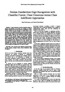
III.1. The Classification Decision Trees Classification Decision Trees (CDT) are a powerful learning classification algorithm (Data mining induction techniques) that is widely used in many applications such as radar signal classification, OCR and expert systems [8]. The DT is based on conditional probabilities that generate a set of hierarchical rules which are successively applied to the input data. It consists of two types of nodes [12]: - A leaf node that indicate labeled of the instances to be classified - An internal decision node that contain an associated splitting predictor (i.e. a prediction criterion). Mostly, binary predicators are used. The CDT is processed in two phases [11]. - The tree building phase: is a top-down strategy, in which training dataset is examined to find the splitting predicator for the root node. Then the same process is made recursively on each child node. Finally, a hierarchical tree structure is generated representing the entire dataset. - The tree pruning phase: in this stage lower branches are removed to improve the performance by minimizing the over-fitting. This performance is measured by an impurity function defined for each node [15]. Fig. 1. represents explained the structure and the possible consequence of CDT.

A=X

A

B

A, B and C =nodes X & Y=conditions A=Y R1, R2 and R3 =labels B

B=X C

C

R1

R2

R3

Fig. 1. Example for a simple decision tree structure

III.2. The Artificial Neuronal Network Artificial Neuronal Network (ANN) has been employed to achieve the mathematical models of biological neurons system. In the recent year ANN has been used in many complex classification problems in business, science, industry and medicine [5]. It consists of a set of connected units (nodes, neurons). Each node has an input and output then it can be connects with other nodes (Figs. 2). Each connection has a weight associated to it. Like any supervised learning method, NN consist of two phase [2]:

International Review on Computers and Software, Vol. 8, N. 6

1229

J. Mtmet, H. Amiri

-

The learning phase: where it adjusts the weights in accordance to the chosen learning algorithm The testing phase: where it predicts the class label of the new input data set.

form of vectors which constitute the input for both classification algorithms. The vectors are of the form: (Image id, class, F1, F2… Fn) where F1…Fn are the n features extracted from a given image.

Figs. 2. Architecture of an artificial neuron and a multilayered neural network [3]

We can define the type of the corresponding ANN based on it [7]: • Topology • Training methodology (learning algorithm) • The connection between the different neurons Multilayer Perceptron Network (MLP) and Radial Basis Function (RBF) network are two of the most ANN used as classifiers. Their architecture consists of three types of layers: an input layer, one or more hidden layers and an output layer [7]. Even though the two classifiers are similar in structural aspect, their mechanisms (type of output layer, the transfer function) are very different. In fact, the RBF have a single hidden layer, whereas MLP can have any number of hidden layers [24]. Moreover, the activation function of the hidden layer in an RBF network computes the Euclidean distance between the input signal vector and parameters vector of the network, whereas the activation function of a multilayer perceptron computes the inner product between the input signal vector and the pertinent synaptic weight vector. In addition the output layer of an RBF network is always linear, whereas in a multilayer perceptron it can be the both linear or nonlinear [24].

IV.

Images

Images

Features extraction

Features extraction

Label

Features Features

Classifier Model (NN/TD)

Machine Learning Algorithm

Label (PHT/TXT/CMP) Prediction

Training

Fig. 3. Implementation strategy of the classification and archiving documents system

For every image, six low-level features are extracted. They are calculated as follows: - Mean: is the average color value in the image:

The Proposed System

Image classification in our proposed system is built on two main stages: off-line image training and on-line image classification. In the training stage, features are automatically extracted from training images data set and linked to categories (photo, textual and compound images) through the training algorithm. Next, in the classification stage, we classify images into one of the categories using the specific classifier (see Fig. 3).

µ =

=


×

(1)

where i represents the color channel and Pij is the probability of occurrence of pixel with intensity j. - Standard deviation: is the square root of the variance of the probability distribution:

IV.1. Features Extraction Feature selection is the cornerstone of the classification task. In fact, features selection is an empiric process, though many approaches are suggested to weight their importance. In our system, the extracted features are automatically stored into a database in the

1

-

1

−µ

(2)

Skewness: represents the measure of the degree of asymmetry in the probability distribution.


1230

J. Mtmet, H. Amiri

1

=

-

(3)

−µ

Entropy: represent the disorder or the complexity of the image. A high value of entropy indicates a complex textures: = −

-

The Artificial Neuronal Network: In our case we used an RBF network. In which the input layer had 6 nodes that are equal to the number of features organized as vectors in the database. For the hidden layer, we chose 6 nodes while the output layer contains three nodes. By the end of this process, an input image is classified either as a photo, a pure text or a compound document (Fig. 5).

(4)

Image dimension: represents the length and width of the image. IV.2. Classification Stage

In our case we used an RBF network. In which the input layer had 6 nodes that are equal to the number of features organized as vectors in the database. For the hidden layer, we chose 6 nodes while the output layer contains three nodes. By the end of this process, an input image is classified either as a photo, a pure text or a compound document. - The Decision Trees: In our paper we fitted the DT to the training data using the cross validation technique in order to select the best tree. Thus, we obtained two tree-based models (original, pruned) that were used in the classification task (Fig. 4).

Features extraction

[1, 0, 0] for photo [0, 1, 0] for text [0, 0, 1] for compound Fig. 5. Flowchart of NN system

V. Features extraction

A data base of 1034 documents was considered for both classification systems. From this set of documents 75% were used for training and 25% for testing the system performance. Thus, the training data set consists of 465 photo including indoor, outdoor, scenes, landscape images documents, 135 textual documents include scanned and computer-generated text in various font and 175 compound documents. Fig. 6 shows some of the class images from the training data set.

Width >= 661

< 661

Stand dev

Pht =-61.30 Txt

Experimental Results

TABLE I DATASETS Class Training Photo 465 Textual documents 135 Compound documents 175

CMP

Testing 155 45 59

Fig. 4. Flowchart of used decision tree (purned)



1231

J. Mtmet, H. Amiri

-

F-measure is the harmonic mean of the recall and precision rate. CCI represents the number of Correctly Classified Images. MI is the number of Misclassified Images and TI is the number of Test Images for each class. The F-Measure was used, because it only produces a high result when Precision and Recall are balanced, thus this is very significant. Table II presents the results obtained by using the Decision Tree, without and with pruning. We can see that only for textual documents the full Decision Tree achieve high F-measure value than the pruned one. TABLE II CLASSIFICATION RESULTS USING DT Full tree

Pruned tree

Recall precision F- Recall precision Frate rate measure rate rate measure Photo Textual documents Compound documents

0,92 0,89

0,85 0,80

0,88 0,84

0,95 0,77

0,90 0,63

0,92 0,70

0,98

0,98

0,98

0,98

0,98

0,98

The ANN’s ability to properly classify documents is shown in Table III for two transfer function. In our model we used the following two networks for classification: 1. Radial Basis Function (RBF) Networks 2. Hyperbolic Tangent Transfer (HTT) function As shown in Table II, HTT classifier achieves the higher values of f-measure than the RBF one only for compound document image class. Whereas, for all the remaining classes RBF is showing high results. TABLE III CLASSIFICATION RESULTS USING NN RBF Transfer function

Hyperbolic tangent Transfer function

Recall precision F- Recall precision Frate rate measure rate rate measure Photo Textual documents Compound documents

Fig. 6. Examples of training data set images

Next we discuss the results obtained after carrying out the classification procedure on the selected. A comparison of the performance of the both classifier has been stated here. The recall rate, precision rate and f-measure are used to evaluate the classification performance for both classifiers. - The recall rate= -

The precision rate=

(

)


0,98 0,68

0,98 0,55

0,98 0,57

0,97 0,70

0,95 0,59

0,96 0,60

0,98

0,98

0,98

0,94

0,89

0,92

These results show that both classifiers achieve notable results in the classification of documents. The DT classifier outperforms the NN classifier in execution speed and Recall value (by 12%). Sample images correctly classified by the both classifier are shown in Fig. 7 (“Photograph images”), Fig. 8 (“Textual document images”) and Fig. 9 (“Compound document images”) There are some cases of misclassification produced by the both classifiers (RBF and pruned classifier). Fig. 10 shows three examples of these images. The main causes of misclassification on text are due to bad lighting conditions and to excessively noisy backgrounds that cause the final uniformity test to fail.


1232

J. Mtmet, H. Amiri

Fig. 7. Photo Images

Fig. 9. Compound document image

Fig. 10. Samples of misclassified images with full Decision Tree classifier

VI.

Conclusion

Automatic classification of documents is a very useful task for building a digital archive management system. The aim of this work is to present an algorithm for

Fig. 8. Textual document image



1233

J. Mtmet, H. Amiri

classifying photo, textual and compounds images. Firstly, features are extracted from images to be assigned to a characteristic vector. Then, in order to train and validate the classification model we used two classifiers (Neuronal Network, Decision Tree). First of all, we have observed that the classification model which uses the DT achieved an average F-measure of 90%, whereas it decreases to 87% for the NN based model. Moreover, we observed that the NN based model have difficulties to classify textual document even though it achieves good result for all the remaining classes. On the other hand, decision trees achieve a good result for all classes. In order to achieve better performance in all categories, we will particularly study other useful highlevel features in order to increase the accuracy of our classification system. In addition, we will look for the integration of new machine learning technique to build a new intelligent classifier.

References [1]

[2]

[3]

[4] [5]

[6]

[7]

[8]

[9]

[10]

[11]

[12]

[13] [14]

A. Jain, and H. J. Zhang, Bayesian framework for hierarchical semantic classification of vacation images, Proceedings of the IEEE International Conference on Multimedia Computing and Systems (ICMSC), pp. 518–523, Florence, Italy, 1999. Ajith Abraham, Artificial Neural Networks, Handbook for Measurement Systems Design, Peter Sydenham and Richard Thorn (Eds.), John Wiley and Sons Ltd., London, pp. 901-908, 2005. Chih-Fong Tsai, On Classifying Digital Accounting Documents, The International Journal of Digital Accounting Research, Vol. 7, N. 13, pp. 53-71, 2007 David Lowe, Distinctive image features from scale-invariant key points. International Journal of Computer Vision, 2004. G.D. Zhang, Neural Network for classification: A Survey, IEEE Transaction on Systems, Man and Cybernetics Part C, Vol. 30, n. 4, pp. 451-462, 2000. Hyontai sug, Performance Comparison of RBF networks and MLPs for Classification, Proceedings of the 9th WSEAS International Conference on applied Informatics and Communications (AIC '09), pp.450-454. 2009 Jay Gao, Decision Tree Image Analysis, Digital Analysis of Remotely Sensed Imagery book, The McGraw-Hill Companies, Inc. pp.351-388, 2009. Kaizhu Huang, Haiqin Yang, Irwin King and Michael Lyu, Global Learning vs. Local Learning, Machine Learning Modeling Data Locally and Globally book, Zhejiang university press and springer, pp. 13-25, 2008. Kaizhu Huang, Haiqin Yang, Irwin King, and Michael R. Lyu, Local Learning vs. Global Learning: An Introduction to MaxiMin Margin Machine, Support Vector Machines: Theory and Applications, pp.177: 113-131, 2005. Kun-Che Lu, Don-Lin Yang, Image Processing and Image Mining using Decision Trees, Journal Of Information Science And Engineering, Vol. 25, pp. 989-1003, 2009. L. Breiman, J. H. Friedman, R. A. Olshen, and C. J. Stone, Classification and Regression Trees. New York: Chapman & Hall, 1984. Lins, R.D. and D.S.A. Machado, A Comparative Study of File Formats for Image Storage and Trans, Journal of Electronic Imaging, Vol. 13 (1), pp. 175-183, 2004. M. M. Gorkani and R. W. Picard, Texture orientation for sorting photos ‘at a Glance, Proc. ICPR, pp. 459–464, Oct. 1994 Matthew N. Anyanwu, Sajjan G. Shiva, Comparative Analysis of Serial Decision Tree Classification Algorithms, International Journal of Computer Science and Security, Vol. 3, Issue 3, pp. 230-240.


[15] Olivier Bousquet, Stéphane Boucheron, Gábor Lugosi, Introduction to Statistical Learning Theory, Advanced Lectures on Machine Learning, pp.169-207, 2003 [16] R. Schettinia, C. Brambillab, G. Cioccaa, Valsasnaa,M. De Pontic, A hierarchical classification strategy for digital documents, Pattern Recognition, vol 35, pp. 1759–1769,2002 [17] Rafael Dueire Lins, Gabriel Pereira e Silva, Brenno Miro, Automatically Deciding if a Document was Scanned or Photographed, Journal of Universal Computer Science, vol. 15, no. 18, pp. 3364-3375, 2009 [18] S. B. Kotsiantis, Supervised Machine Learning: A Review of Classification Techniques, Informatica journal, Volume 31, Number 3, pp. 249-268, 2007. [19] S. Prabhakar, H. Cheng, J.C. Handley, Z. Fan Y.W. Lin, Picturegraphics Color Image Classification, Proc. of ICIP, pp. 785-788, 2002. [20] S.J. Simske, Low-resolution photo/drawing classification: metrics, method and archiving optimization, Proceedings IEEE ICIP, IEEE, Genoa, Italy, pp. 534-537, 2005. [21] Soo Beom Park, Jae Won Lee, Sang-Kyoon Kim, Content-based image classification using a neural network, Pattern Recognition Letters, Volume 25, Number 3, pp.287-300, 2004 [22] V. Athitsos, M. J. Swain, and C. Frankel, Distinguishing Photographs and Graphics on the World Wide Web, in IEEE Workshop on Content-Based Access of Image and Video Libraries, pp. 10-17, June 1997. [23] Y. Bouzida and F. Cuppens, Neural networks vs. decision trees for intrusion detection, In IEEE/ISTWorkshop on Monitoring, Attack Detection and Mitigation (MonAM), 2006. [24] Huang, N., Liu, X., Xu, D., Lin, L., Power quality disturbances recognition based on Hyperbolic S-transform and rule-based decision tree, (2011) International Review of Electrical Engineering (IREE), 6 (7), pp. 3152-3162.

Authors’ information 1

Signal, Image and Technologies of Information Laboratory, National Engineering School of Tunis, Tunis el Manar University, BP 37 Belvedere, 1002, Tunis, Tunisia. E-mail: [email protected] 2

Signal, Image and Technologies of Information Laboratory, National Engineering School of Tunis, Tunis el Manar University, BP 37 Belvedere, 1002, Tunis, Tunisia. E-mail: [email protected] Jassem Mtimet was born in zarzis TUNISIA. He is PhD student at the National School of Engineer of Tunis (ENIT-Tunisia). He received his master’s degree in Automatic and Signal Processing from ENIT. Bachelor’s degree in Computer Science from Faculty of Sciences of Tunis. His doctoral study focused on the document image analysis. Hamid Amiri received the Diploma of Electrotechnics, Information Technique in 1978 and the PhD degree in 1983 at the TU Braunschweig, Germany. He obtained the Doctorates Sciences in 1993. He was a Professor at the National School of Engineer of Tunis (ENIT), Tunisia, from 1987 to 2001. From 2001 to 2009 he was at the Riyadh College of Telecom and Information. Currently, he is again at ENIT. His research is focused on • Image Processing. • Speech Processing. • Document Processing. • Natural language processing


1234


Cluster Based Reliable Forwarding Mechanism for Data Dissemination in Vehicular Ad Hoc Networks S. Lakshmi1, R. S. D. Wahida Banu2 Abstract – In Vehicular Ad Hoc Networks (VANET), the efficient data dissemination is affected by the critical factors such as connectivity, transmission quality and redundancy elimination. Most of the existing techniques concentrate either on sparse or dense populated vehicular network that increases redundancy. Though existing clustering technique improves the connectivity, there is lack in transmission quality. In order to overcome these issues, in this paper, we propose a cluster based reliable forwarding mechanism for Data dissemination in vehicular networks. In this technique, the multilane two way highway is divided into clusters based on the deployment of road side units. Within the clusters, the node with highest transmission quality is selected as the cluster head based on the transmission quality. The cluster head uses the backfire algorithm for data transmission that minimizes the redundancy in the network. By simulation results we show that the proposed technique minimizes the redundancy and improves the reliability. Copyright © 2013 Praise Worthy Prize S.r.l. - All rights reserved.

Keywords: Vehicular Ad Hoc Networks (VANET), Data Dissemination Packet Error Rate (PER)

Ad Hoc network containing set of vehicles communicating between each other in ad hoc mode using the wireless medium. The vehicles move on a predefined path due to road topology and at the same time have high speeds. The kind of communication between vehicles is called “Inter- Vehicular Communications”. In addition to communicating among themselves, the vehicles also communicate with fixed units on the road also known as Road Side Units (RSUs) [1]. The communication modes include the self-organizing multi-hop communication of node to node and the communication of nodes to RSU. Vehicular Ad-hoc Networks that is one of the sensor networks and wireless ad hoc networks is a special application in the field of intelligent transportation. It has some new significant features: a large scale network, fast moving nodes, non-uniform spatial distribution of nodes, node trace restricted by the path, the nodes with strong computing power and adequate power supply. Typical applications of VANET include traffic management, traffic safety and urban monitoring [2] [16], [19].

Nomenclature PER Prx Ptx   d  h SNR  P iin BER FER L N Twait Tmw R dn dp V (t) () a(t)

Packet Error Rate Received signal power Transmission Power Wavelength of the propagating signal Reflecting coefficient of the ground surface Distance among the transmitter and receiver Path loss factor Antenna height Signal to Noise Ratio Background noise Interference of neighbor i Bit Error Rate Frame Error Rate Bit length of each frame Total number of retransmission times Waiting time Maximum waiting time Transmission Range Shortest distance from node i to destination Shortest distance from packet forwarding source to destination Node’s speed at time t Random value in the interval [-1, 1] Acceleration of the node at time t

I. I.1.

I.2.

Architecture of VANET

The automobile industries are working hard to enhance the vehicles’ safety features by taking advantage of on-board sensor technologies [17]. VANET is a sensor based technique in which wireless communication on board enable communication between, Vehicles-toVehicles (V2V) and Vehicles-to-Infrastructure (V2I). With VANET, vehicles can communicate on the live update of traffic, road signal and emergency circumstances.

Introduction

Vehicular Ad Hoc Network (VANET)

Vehicular Ad Hoc Network (VANET) is a Dynamic



1235

S. Lakshmi, R. S. D. Wahida Banu

Wi-Fi is used as the communication medium, in which data transmission is at high speed at short interval of time. The concept of these driver-aids systems is that, by using the information collected by the sensors on the vehicle, potential unsafe situations could be detected rapidly and automatically; and these captured data could alert the driver or help the driver with appropriate actions. [5] If the vehicles are provided with updated information regarding road traffic conditions, informed and intelligent decision help to take right actions to avoid being trapped in heavy traffic jams. In the existence of infrastructures or road side units, two data dissemination approaches are assumed: push-based and pull-based. In the push-based approach, data is disseminated to anyone and suitable for popular data. In pull-based approach request-reply methodology is used and suitable for unpopular data propagation. With lacking of infrastructure two dissemination approaches can be considered: flooding and relaying [6]. Components of VANET  Sensing Peripherals,  Alert Peripherals,  Data Processing and Fusion Unit,  Local Dynamic Map (LDM),  Applications,  Message Manager [3]. I.3.

Features of VANET

There are several important factors, which make VANET type of networks specific and which allow treating them as a separate category. Here are the fundamental VANET features:  Very high dynamics of nodes resulting in fast topology changes. As the communication devices are installed inside vehicles, the network nodes are much more mobile and they move with much higher speeds. Vehicles are restricted to move using roads and to abide by the traffic rules, so some mobility patterns can be observed and some statistical mobility models for VANET have been designed.  Information about the current position, movement direction, current velocity, city map and planned movement trajectory of VANET nodes is available, as more and more vehicles are equipped with GPS devices and navigation systems.  VANETs impose lack of energy constraints, higher computational power and practically unlimited memory capacity, in comparison to some other ad hoc networks (especially to sensor networks like MANET).  VANET networks are usually of very large size (case of traffic jams) but also may exist in a form of many small, neighboring networks with a high probability of splitting and joining.  There is a big diversity of VANET services and applications, and one-to-one communication is less important than some intelligent broadcast (for Copyright © 2013 Praise Worthy Prize S.r.l. - All rights reserved

example geocast) required by most safety related applications. [4] I.4.

Data Dissemination in VANET

The data dissemination is the working method involved in VANET. Data dissemination involves both V2I and V2V in which push, pull, flooding and relaying are used for communication. I.4.1. Vehicle to Infrastructure (V2I) Push-based and Pull-based approaches are considered for V2I data dissemination. a. Push-Based Approach In the push-based approach, the roadside unit broadcast the data to all vehicles which are in its range. Disadvantage is that everybody may not be interested to the same data. It is suitable for applications supporting local and public-interest data such as data related to unexpected events or accidents causing congestion and safety hazards. It also generates low contentions and collisions during packet propagation. b. Pull-Based Approach In pull based approach vehicles are enabled to query information about specific targets and responses are routed toward them. It is useful for acquiring individual specific data. It generates a lot of cross traffics including contentions and collisions during packet propagation. It is noted that periodically pouring data on the road is necessary since vehicles receiving the data may move away quickly, and vehicles coming later still need the data. The proposed model consists of communication between vehicles and fixed infrastructures named as parking automat and also between vehicles [6]. I.4.2. Vehicle to Vehicle (V2V) Flooding and relaying are two approaches that can be considered for vehicle to vehicle data dissemination. a. Flooding Approach In the flooding mechanism all types of data is broadcasted to neighbors. Whenever another vehicle receives a broadcast message, it stores and immediately forwards it by rebroadcast. It is suitable for delay sensitive applications and also for sparsely connected or fragmented networks. This mechanism is not scalable and generates broadcast storm problem due to high message overhead during rush hours or traffic jams. b. Relaying Approach In the relaying mechanism relay node is selected for disseminating the messages. The relay node is responsible for forward the packet further. In this approach contention is less and it is scalable for dense networks. This is due to the less of number of the nodes


1236


participating in forwarding message and as a result generated overhead is less [6]. I.5.

Routing in VANET

Routing in VANET, enable congestion free, easy access communication between two vehicles when they are near at particular range. Some of the proposed routing protocols are GSR, A-STAR, GPCR and GyTAR:  Geographic Source Routing (GSR),  Anchor-based Street and Traffic Aware Routing (ASTAR),  Improved Greedy Traffic Aware Routing protocol (GyTAR) [7].

connectivity, transmission quality and redundancy elimination are the critical factors. In ACAR [11], performance on highly dynamic vehicle network is degraded hence the method can be adapted only for sparsely vehicular network. Moreover it does not reduce redundancy. Backfire algorithm is efficient for densely populated vehicular network hence it can only be implemented in urban areas [1]. Also connectivity and transmission quality are not considered. In [13], clustering is used to ensure the connectivity but transmission quality and redundancy elimination are ignored. To overcome the above issues, we formulate a cluster based reliable forwarding mechanism for Data dissemination in vehicular networks.

II. I.6.

Advantages of Using VANET

 When a car passes by a sensor network, it retrieves fresh environmental data collected by the roadside sensors enabling the driver to get update of the road traffic in the near distant.  External sensor networks data can include various physical quantities, such as temperature, humidity and light, and also detect moving obstacles (such as animals) which gives an alert for driver than wireless sensor nodes installed in vehicles.  Accidents due to blind curve and unmanned railway cross can also be reduced to an extent [8]. I.7.

Issues Caused in VANET

 Due to high mobility, the connectivity among nodes could last only few seconds, and fail in unpredictable ways.  Maintaining end-to-end connectivity, packet routing, and reliable multi-hop information dissemination will become extremely challenging.  The strong interference and collision related to the high number of mobile transmitters (vehicles).  The flapping links, caused by fading effect and vehicles' speed [9].  The uneven distribution of vehicles on the roads makes route selection more complex.  Some protocols make use of the density information on roads to select routes; but the inaccurate statistical data may cause route paths to be wrongly computed.  Because of the blocking of wireless signal by objects, e.g. skyscraper in the city, communication between vehicles must have the line-of-sight [11].  VANETs are based on short-range wireless communication hence communication should be fast enough to transfer data at a particular interval of time [13]. I.8.

Problem Identification

Generally for efficient data dissemination in VANET,


Related Works

Nestor Mariyasagayam et al [1] have proposed an adaptive forwarding scheme. Improvements obtained in efficiently disseminating information over VANET were shown. The adaptive mechanism which uses a dynamic backfire algorithm dynamically adjusts the area within which the forwarders have to be refrained from sending a particular message based on the density of neighbors. Overall, a 5% to 25% increase is seen in comparison with the non-adaptive scheme and much more when compared with flooding. Wang Ke et al [2] have proposed a data dissemination strategy which is called the Adaptive Connectivity Data Dissemination Scheme (ACDDS). The nodes calculate the network connectivity in current areas by the distributed nodes density perception algorithm. Then hop limit function is established on the basis of the Euclidean distance and nodes density between the nodes and hotspot, meanwhile, the hop count of the message transmitted will be limited dynamically in order to reduce the duplication of message copies in the hotspot areas, according to which, the number of redundant massages copies will be reduced effectively. Moez Jerbi et al [10] have proposed an inter-vehicle ad-hoc routing protocol called GyTAR (improved Greedy Traffic Aware Routing protocol) suitable for city environments. GyTAR consists of two modules: dynamic selection of the junctions through which a packet must pass to reach its destination and an improved greedy strategy used to forward packets between two junctions. The approach present its added value compared to other existing vehicular routing protocols. Qing Yang et al [11] have proposed an adaptive connectivity aware routing (ACAR) protocol that addresses these problems by adaptively selecting an optimal route with the best network transmission quality based on the statistical and real-time density data that are gathered through an on-the-fly density collection process. The protocol consists of two parts: 1) select an optimal route, consisting of road segments, with the best estimated transmission quality 2) in each road segment in the selected route, select the most efficient multi-hop path that will improve delivery ratio and throughput.


1237


The optimal route can be selected using our new model that takes into account vehicles densities and traffic light periods to estimate transmission quality at road segments, which considers the probability of connectivity and data delivery ratio for transmitting packets. In each road segment along the optimal path, each hop is selected to minimize the packet error rate of the entire path. Josiane Nzouonta et al [12] have proposed Road-Based using Vehicular Traffic information routing (RBVT) protocols use real-time vehicular traffic information to create road-based paths between end-points. Geographical forwarding is used to find forwarding nodes along the road segments that form these paths. To improve the end-to-end performance under high contention, proposed a distributed next hop self-election mechanism for geographical forwarding. Because the RBVT protocols forward data along the streets, not across the streets, and take into account the real traffic on the roads, they perform well in realistic vehicular environments in which buildings and other road characteristics such as dead end streets are present. Pratibha Tomar et al [13] have proposed approach for data dissemination for highway scenarios for vehicular networks. Used a roadside units, and clusters formation in the proposed approach. In the proposed architecture V2V and V2I communication was done according to information priority. The architecture for data dissemination in VANETs is also proposed. The main advantage of using roadside units in our approach is to achieve low latency communication within vehicles and it can be extended in terms of their connectivity. This approach is also useful for distributing time critical data. Nisha K.Warambhe and Dr. S. S. Dorle [14] has proposed that the system will consists of one control node as a roadside unit and two mobile nodes as an onboard unit. Data is disseminated between the mobile nodes via control node using push-based V2V/V2I dissemination technique, and then data which is disseminated through control node in all mobile nodes are stored into the memory of AVRATMEGA32. Stored data can be retrieved for analysis of accident cause or any emergency situation occurs. Analog to digital conversion is required during disseminating data between control node and mobile node. The parameters used for the verification of data dissemination and data storage are Temperature, Location of vehicle and accident cause which depends on the event occurred at the node. Also a hardware model is designed which uses AVR ATMEGA32 micro-controller and RF Trans-receiver module and WINAVR and Cygwin is used for programming.

III. Problems and Proposed Solution

In this technique, the multilane two way highway is divided into clusters based on the deployment of road side units. Within the clusters, the node with highest transmission quality is selected as the cluster head based on the transmission quality. The cluster head uses the backfire algorithm for data transmission that minimizes the redundancy in the network. III.2. Estimation of Metrics III.2.1. Estimation of Packet Error Rate (PER) In our technique, we select the cluster head based on transmission quality which is estimated using Packet error rate (PER) [11]. The estimation of PER involves the following sequential steps. 1) Computation of received signal power (Prx) in the line of sight (LOS): Prx 

  4 h 2 2 1    2 cos  d    d  4 2      Ptx



    

(1)

where: Ptx = transmission power, d = distance among the transmitter and receiver,  = wavelength of the propagating signal,  = reflecting coefficient of the ground surface,  = path loss factor, h = antenna height. 2) Computation of Signal to Noise Ratio (SNR):   Prx SNR =  . log10   i     Pin   

(2)

where:  = background noise; P iin = interference of neighbor i;  = constant. 3) The signal is modulated using the Bit error rate (BER) which is computed using Eq (3): BER = z ( 2  SNR )

(3)

where:

 x  z(x) = 0.5 - 0.5 · c    2 c = error function. 4) Computation of frame error rate (FER) of the link (Li): N

III.1. Overview In this paper, we propose a cluster based reliable forwarding mechanism for Data dissemination in vehicular ad hoc networks.


FERLi = 1-

 1  FER  FERi

(4)

i 0

where FER = 1- (1- BER)L


1238


L = bit length of each frame; N = total number of re-transmission times. 5) If packet contains r frames, the packet error rate (PER) is computed using Eq (5): PER = 1 – (1 - FERLi)r

(5) III.3. Proposed Architecture

6) If there are j route with n hops, then PER of a road segment for forwarding packets along these hops is given using Eq (6): n

PERRS = 1-

 1  PER 

(6)

1

III.2.2. Estimation of Waiting Time The node after knowing its own position, determines a waiting time (Twait) based on the distance to the source node [6]. The waiting time is minimum for distant receivers. Twait is estimated using the following Eq. (7):

Twait 

Tmw   d  Tmw R

d  min d ,R

where V (t) = node’s speed at time t  ( ) = random value in the interval [-1, 1] a(t) = acceleration of the node at time t.

Fig. 1 demonstrates the multilane two way highway architecture. C1, C2, C3 represents the clusters and {Na,Nb,Ne,Nh,Ni,Nl}, {Nc,Nf,Nj,Nm} and {Nd,Ng,Nk,Nn} are the cluster member nodes. Each node is enabled with global positioning system (GPS). The two category of message involved in the communication among the nodes are as follows. 1) Direct or emergency message 2) Normal communication message Within the different clusters, the security message can be broadcasted from road side unit (RSU) which is obtained from the cluster head or nodes.

(7) (8)

where Tmw = maximum waiting time: R = transmission range; d = distance from sender Fig. 1. Proposed Architecture of VANET

III.2.3. Node Distance Using the information received from the GPS receivers, the location and distance information of the nodes can be estimated. This information is communicated to neighbor nodes using beacon messages. This helps in computing the neighbor node near to the destination node using the following Eq. (9) [15]:

 d d  1  n  dp 

   

(9)

where: dn = shortest distance from neighbor node i to destination dp = shortest distance from packet forwarding source to destination:

dn  = closeness of the next hop dp III.2.4.

Node Speed

The speed of the node is estimated using the freeway technique shown in Eq. (10) [9]: S (t+1) = S (t) +  ( ) · a (t)

(10)


III.3.1.

Cluster Formation

The cluster formation involves the following steps 1) The multilane two way highway is divided into clusters and it is formed based on the RSU. i.e. the specific geographical region to which any RSU broadcasts the information (for that geographical area) on the highway forms a cluster. Each Node within the cluster maintains its information whose format is as shown in Table I. The parameters in the table include node ID, sequence number, node location, node speed and timestamp (Estimated in section 3.2). Node ID

TABLE I NODE MESSAGE FORMAT Sequence Node Node Number location Speed

Timestamp

2) The above information is shared by RSU that makes decision about which node will carry the data packet to destination as per the speed. Step 2 reveals that the sharing of cluster information by RSU is essential as the node can change their cluster and the information needs to be updated in RSU time to time. 3) Each cluster selects a cluster head (CH) based of transmission quality which is estimated using PER


1239


(Estimated in section 3.2). The node with highest transmission quality is selected as the cluster head. 4) The cluster head helps in the transmitting the data to other clusters (Data transmission described in next section). III.3.2. Data Dissemination In order to distribute the data to destined cluster member nodes, we consider Backfire algorithm into consideration. This technique helps in flooding the data in efficient manner among source and destination. The steps involved in the backfire algorithm is as follows: 1) The nodes store the information in its local cache. (Shown in Table I); 2) The receiver node computes the distance among the source node from which the packet originated and itself: If d > Th then: Node prevents transmission Else Go to step 3; 3) Compute the distance among the neighbor node and itself; 4) Based on the distance from the source of the received packet, the delay is computed. As a result, the nodes that are far away waits for minimum waiting time (Twait) (Described in section 3.2.2) and re-transmits the packet quickly when compared to the nodes nearer to source node. 5) If the node receives the same packet more than once, it calculates the relative position of the source again. If the node is located within the cluster, it cancels retransmission of the packet. Fig. 2 demonstrates the data transmission based on Backfire Algorithm. We consider that the cluster head CHa wants to broadcast the message M to nodes Ne and Nb. Ne and Nb sets Twait in order to forward M received from CHa.

1 , Nb will forward M obtained from CHa d prior than Ne. After receiving M from CHa, Ne prevents itself from forwarding M whereas drops the message. Then Ne is said to be backfired by Nb. This algorithm maintains the low latency within the vehicles and minimizes the redundancy. As Twait 

IV.

Simulation Results

IV.1.

Simulation Parameters

The proposed Cluster Based Reliable Forwarding Mechanism (CBRF) is simulated using NS2 [16]. In this simulation, the channel capacity of mobile hosts is set to the value of 2 Mbps. In the simulation, the number of nodes is 78. The mobile nodes move in a 2500 meter x 700 meter square region for 20 seconds simulation time. In our simulation, the data transmission rate is varied from 250kb to 1000kb. The simulation topology is summarized as below.

Fig. 3. Simulation Topology

The simulation settings summarized in Table II.

and

parameters

are

TABLE II SIMULATION PARAMETERS No. of Nodes 78 Area 2500 × 700 MAC 802.11 Simulation Time 20 s Traffic Source CBR Rate 250kb to 1000kb Packet Size 512 bytes Routing Protocol AFM Antenna Type Omni Antenna Mac 802.11

IV.2. Performance Parameters We compare the CBRF with the AFM [1] technique. We evaluate performance of the CBRF mainly according to the following parameters. Control overhead: The control overhead is defined as the total number of routing control packets normalized by the total number of received data packets. Average end-to-end delay: The end-to-end-delay is averaged over all surviving data packets from the sources to the destinations.

Fig. 2. Backfire Algorithm based Data Transmission



1240


Rate Vs Overhead(Scen-1) 30000 Overhead

Average Packet Delivery Ratio: It is the ratio of the number of packets received successfully and the total number of packets transmitted. Throughput: It is the number of packets received by the receiver. The simulation results are presented in the next section.

20000

CBRF

10000

AFM

0 250

500

For scen-1 Based on Rate In this experiment we vary the transmission rate as 250, 500, 750 and 1000kb. From Fig. 4, we can see that the delivery ratio of our proposed CBRF is higher than the existing AFM protocol. From Fig. 5, we can see that the delay of our proposed CBRF is less than the existing AFM protocol. From Fig. 6, we can see that the throughput of our proposed CBRF is higher than the existing AFM protocol. From Fig. 7, we can see that the overhead of our proposed CBRF is less than the existing AFM protocol. Rate Vs DeliveryRatio(Scen-1)

1000

Fig. 7. Rate Vs Overhead

For scen-2 Based on Rate In this second scenario also we are varying the transmission rate as 250,500,750 and 1000kb. From Fig. 8, we can see that the delivery ratio of our proposed CBRF is higher than the existing AFM protocol. From Fig. 9, we can see that the delay of our proposed CBRF is less than the existing AFM protocol. From Fig. 10, we can see that the throughput of our proposed CBRF is higher than the existing AFM protocol. Rate Vs DeliveryRatio(Scen-2)

1 CBRF

0.5

DeliveryRatio

DeliveryRatio

750

Rate(Kb)

IV.3. Simulation Results

AFM

0 250

500

750

1000

0.6 0.4

CBRF

0.2

AFM

0

Rate(Kb)

250

500

750

1000

Rate(Kb)

Fig. 4. Rate Vs Delivery Ratio Fig. 8. Rate Vs Delivery Ratio Rate Vs Delay(Scen-1) Rate Vs Delay(Scen-2)

6

8

CBRF

4

Delay(Sec)

Delay(Sec)

8

AFM

2 0 250

500

750

1000

6

CBRF

4

AFM

2 0 250

Rate(Kb)

500

750

1000

Rate(Kb)

Fig. 5. Rate Vs Delay Fig. 9. Rate Vs Delay Rate Vs Throughput(Scen-1)

CBRF

Throughput

Throughput

Rate Vs Throughput(Scen-2) 10000 8000 6000 4000 2000 0

AFM

250

500

750

1000

6000 4000

CBRF

2000

AFM

0 250

Rate(Kb)

500

750

1000

Rate(Kb)

Fig. 6. Rate Vs Throughput Fig. 10. Rate Vs Throughput



1241


From Fig. 11, we can see that the overhead of our proposed CBRF is less than the existing AFM protocol.

[9] [10]

Rate Vs Overhead(Scen-2)

Overhead

30000 20000

CBRF

10000

AFM

[11]

0 250

500

750

1000

[12]

Rate(Kb)

Fig. 11. Rate Vs Overhead

V.

[13]

Conclusion

[14]

In this paper, we have proposed a cluster based reliable forwarding mechanism for Data dissemination in vehicular networks. In this technique, the multilane two way highway is divided into clusters based on the deployment of road side units. Within the clusters, the node with highest transmission quality is selected as the cluster head based on the transmission quality. The cluster head uses the backfire algorithm for data dissemination that minimizes the redundancy in the network. By simulation results we have shown that the proposed technique minimizes the redundancy and ensure reliable data transmission in VANET.

[15]

[16]

[17]

[18] [19]

References [1]

[2]

[3]

[4]

[5]

[6]

[7]

[8]

Nestor Mariyasagayam, Hamid Menouar, Massimiliano Lenardi and Hitachi Europe Sas, “An Adaptive Forwarding Mechanism for Data Dissemination in Vehicular Networks”, Vehicular Networking Conference (VNC), 2009 IEEE. Wang Ke1, Yang Wei-dong, Liu Ji-zhao and Zhang Dan-tuo, “An Adaptive Connectivity Data Dissemination Scheme in Vehicular Ad-hoc Networks”, 2011 Seventh International Conference on Computational Intelligence and Security. Filippo Visintainer, Fabien Bonnefoi, Francesco Bellotti and Tobias Schendzielorz, “Infrastructure-Based Co-Operative Architectures: How Safespot Deals With Different Road Network Areas”, 14th World Congress and Exhibition on Intelligent Transport Systems and Services, Beijing, China [Boneo 2007]. Sławomir Kukliński and Grzegorz Wolny, “CARAVAN: ContextAwaRe Architecture for VANET”, Published on 30. January, 2011, Mobile Ad-Hoc Networks: applications, Xin Wang (Ed.), ISBN: 978-953-307-416-0, In Tech. Hemjit Sawant, Jindong Tan and Qingyan Yang, “A Sensor Network Approach for Intelligent Transportation Systems”, In (IROS 2004). Proceedings. 2004 IEEE/RSJ International Conference on Intelligent Robots and Systems, 2004. Dharmendra Sutariya and Dr. S. N. Pradhan, “Data Dissemination Techniques in Vehicular Ad Hoc Network”, International Journal of Computer Applications (0975 – 8887), Volume 8– No.10, October 2010. Shahzad Ali and Sardar M Bilal, “An Intelligent Routing Protocol for VANETs in City Environments”, Computer, Control and Communication, 2009. IC4 2009. 2nd International Conference on 17-18 Feb. 2009. Andreas Festag, Alban Hessler, Roberto a, Long Le, Wenhui Zhang and Dirk Westhoff, “Vehicle-To-Vehicle And Road-Side Sensor Communication For Enhanced Road Safety”, In ITS World Congress (2008) Key: citeulike:6634000.


Gianluca Grilli, “Data dissemination in vehicular networks”, Technical Report, June 2010. Moez Jerbi, Sidi-Mohammed Senouci, Rabah Meraihi and Yacine Ghamri-Doudane, “An Improved Vehicular Ad Hoc Routing Protocol for City Environments”, This full text paper was peer reviewed at the direction of IEEE Communications Society subject matter experts for publication in the ICC 2007 proceedings. Qing Yang, Alvin Lim, Shuang Li, Jian Fang and Prathima Agrawal, “ACAR: Adaptive Connectivity Aware Routing Protocol for Vehicular Ad Hoc Networks”, Computer Communications and Networks, 2008. ICCCN '08. Proceedings of 17th International Conference on 3-7 Aug. 2008. Josiane Nzouonta, Neeraj Rajgure, Guiling Wang and Cristian Borcea, “VANET Routing on City Roads using Real-Time Vehicular Traffic Information”, Vehicular Technology, IEEE Transactions on Sept. 2009. Pratibha Tomar, Brijesh Kumar Chaurasia and G. S. Tomar, “State of the Art of Data Dissemination in VANETs”, International Journal of Computer Theory and Engineering, Vol.2, No.6, December, 2010. Nisha K.Warambhe and Dr. S.S. Dorle, “Implementation of Protocol for Efficient Data Storage and Data Dissemination in VANET”, International Journal of Advanced Research in Computer Science and Electronics Engineering, Volume 1, Issue 2, April 2012. K. Prasanth and K. Duraiswamy, “Minimizing End to End Delay in VANETs using Potential Edge Node Based Greedy Routing Approach”, European Journal of Scientific Research, pp.631-647, Vol.48 No.4, 2011. Xu, H., Zhou, L., Consistence-based detection location verification for VANETS, (2012) International Review on Computers and Software (IRECOS), 7 (4), pp. 1900-1905. Zhou, Z., Jing, Z., Ma, L., Zhu, F., Evaluation of Metropolis Commuter rail-transportation transit vehicle planning based on grey weighting relation method, (2012) International Review on Computers and Software (IRECOS), 7 (5), pp. 2461-2465. Network Simulator: http:///www.isi.edu/nsnam/ns Rabindra Ku Jena, Developments in Vehicular Ad-Hoc Network, (2013) International Review on Computers and Software (IRECOS), 8 (3), pp. 710-721.

Authors’ information Ms. S. Lakshmi received her B.Sc degree in Mathematics from Madras University and Masters in Computer Application from the same University. She is pursuing her PhD from Anna University. She is member of IEEE .She is currently working as Senior Assistant Professor in Department of Computer Applications, Sona College of Technology, Salem. Her area of includes Vehicular Adhoc Networks, Data Mining especially Text Mining using Predictive analytics, Knowledge Management and Image Processing. She is currently working on a sponsored project of AICTE on Text Mining Dr. R. S. D. Wahida Banu has obtained her Bachelor degree in Electronics and Communication from Madras University, Chennai. Then she obtained her Masters degree in Applied Electrinics and PhD in Engineering from the same University in Image Processing. She is the life memebr of ISTE, CSE, Institute of Engineer as well executive member of Salem Chapter, Systems Society of India, VDAT, ISOC and Member of International Association of Engineers. Her specialization includes Image processing, Network security, Adhoc Networks, VLSI, Data Mining and Knowledge Management. She has many awards to her credit like Best Women Engineer, Best Professor Award, Life Time Achievement Award and Best Alumnus Award. She is currently working as the First Women Principal of Salem Government Engineering College


1242


Tumor, Edema and Atrophy Segmentation of Brain MRI with Wavelet Transform and Semantic Features K. Selva Bhuvaneswari, P. Geetha Abstract – MRI Brain Image Segmentation is one of the difficult and complex techniques in the medical field. Normally the pathological tissues such as Tumor and Edema are easily segmented. In this paper, both the normal tissues such as WM (White Matter), GM (Gray Matter) and CSF (Cerebrospinal Fluid) and the pathological tissues such as Tumor, Edema and also Atrophy in the MRI Brain Images are segmented effectively. Initially, the Wavelet Transform features and the Semantic feature from the MRI Brain Images are extracted in two different ways. These extracted features are the input to the next process. Then the proposed segmentation technique performs classification process by utilizing a dual Artificial Neural Network. The ANN is helpful for classifying whether the image is normal or abnormal. Based on the results, the segmentation is carried out. In Segmentation, the normal tissues such as WM, GM and CSF are segmented from the normal MRI images and pathological tissues such as Tumor, Edema and Atrophy are segmented from the abnormal images. The implementation result shows the efficiency of proposed tissue segmentation technique in segmenting the tissues accurately from the MRI images. The performance of the segmentation technique is evaluated by performance measures such as accuracy, specificity and sensitivity. Copyright © 2013 Praise Worthy Prize S.r.l. - All rights reserved.

Keywords: Segmentation, Pathological tissues, Artificial Neural Network, White Matter, Gray Matter, Cerebrospinal Fluid, Tumor, Edema, Atrophy

c X 

Nomenclature bi

Block in image i

EDij

Euclidean distance measure

 i'

Semantic features

H i' , Vi' , Di'

2D Wavelet features

HU a

Hidden units in FFBNN

f1 , f 2

Output unit of FFBNN

  Active  X i'      LE BP E  IS IG

 I G  x, y 

EM IK I wg

Morphological Closing operation applied image

c X h   x, y 

Centroid value for each region

t  x, y 

Tumor centriod value

Oh  x, y 

c Distance between X h   x, y  & t  x, y 

Ie

Edema Segmented image

I. Activation function

The front most part of the central nervous system is the brain. Beside with the spinal cord, it structures the Central Nervous System (CNS). The Cranium, a bony box in the skull guards it. Practically all we do, think, act, reason, walk, talk, the list is continual is since of our brain. The maladies caused in the brain are Brain Tumors. The tumors that nurture in the brain are Brain tumors. A strange development caused by cells reproducing themselves in an unrestrained way is known as Tumor. A gentle brain tumor contains benign (harmless) cells and has separate boundaries. Operation only may heal this kind of tumor. A malevolent brain tumor is serious. As malignant brain tumor contains cancer cells, or it may be called malignant because of its position.

Learning Rate of FFBNN Back Propagation Error Skull Stripped image Smoothed image Gradient of two variables Edge Marked Image Binarized Image WM , GM Segmented image

I CSF

CSF Segmented image

IA

Abnormal MRI images

IT

Tumor Segmented image

Introduction



1243

K. Selva Bhuvaneswari, P. Geetha

A malevolent brain tumor created of cancerous cells may widen or seed to other positions in the brain or spinal cord. It can attack and demolish healthy tissue hence it can never function accurately. By means of Magnetic Resonance Imaging (MRI), the configuration and function of the brain can be learned noninvasively by doctors and researchers. The MRI image is really a lean horizontal piece of the brain. The white region at lower left is the cancer. It appears white since MRI scans increase tissue differences. The cancer is really on the right side of the brain. Lately, to examine the relation between white matter growth and neural maladies, several people exploit the MRI data , particularly, the anatomy image is combining with those images from diffusion tensor imaging, and by the white matter to lead the fibre staple [1]-[2], the precision of fragmenting white matter is main problem. To fragment white matter, Attention deficit hyperactivity disorder (ADHD) [3] is moreover required. Despite many algorithms for fragmenting MRI of data [4-8], for instance watershed algorithm, eSneke algorithm, generic algorithm. Besides, those algorithms are based on the homogeneity of image. Actually, we have to work out the problem with novel method and force inhomogeneity is bang on each image. Based on the expectation-maximization (EM) algorithm, Wells [9] progressed a novel statistical strategy but the results are too reliant on the early values, very consuming the time and now appearing for limited maximum point. Concerning one or more features, the fundamental objective in fragmentation process is to divide an image into areas that are uniform [10]. Fragmentation is an essential device in medical image processing and it has been constructive in several applications, such as: detection of tumors, detection of the coronary border in angiograms, surgical planning, measuring tumor volume and its response to therapy, automated classification of blood cells, detection of micro calcifications on mammograms, heart image extraction from cardiac cine angiograms, etc [11]-[14]. It may be helpful to categorize image pixels into anatomical areas in various applications, such as bones, muscles, and blood vessels, though in others into pathological areas, such as cancer, tissue deformities, and multiple sclerosis lesions. To separate perfectly the whole image into sub areas is the goal in magnetic resonance (MR) images processing, integrated gray matter (GM), white matter (WM) and cerebrospinal fluid (CSF) spaces of the brain [15]. For instance, in a number of neurological turmoil such as multiple sclerosis (MS) and Alzheimer’s disease, the capacity varies in total brain, WM, and GM can give main data about neuronal and axonal loss [16]. A lot of algorithms have been suggested for brain MRI segmentation in latest years. The most famous techniques are integrated thresholding [8], regiongrowing [9] [33], and clustering. The complete computerized intensity-based algorithms have elevated sensitivity to different noise relics such as intra-tissue noise and inter-tissue intensity difference reduction.


Thresholding is extremely plainness and competence. If the objective is obviously apparent from background, the force histogram of the image is bimodal and it can easier get to the optimal threshold by merely selecting the valley bottom as the threshold point. Though, in most of genuine images, there are not obviously discernible marks among the target and the background. Grouping is most famous strategy for fragmentation of brain MR images and usually executes enhanced than the other methods [10]. The remaining of the paper is categorized as follows: a short analysis of some of the literature works in the MRI Brain Image Segmentation is offered in Section 2. The inspiration for this study is specified in Section 3. Section 4 enlightens the short notes for the suggested methodology and the structure for the suggested methodology. The experimental results and presentation study discussions are given in Section 5. At last, the endings are summed up in Section 6.

II.

Literature Survey

For the brain image fragmentation, several researches have been suggested by researchers. A short assess of a few of the recent researches is offered here. Based on adaptive mean-shift clustering in the combined spatial and intensity feature space, an automated segmentation structure for brain MRI volumes has been offered by Arnaldo Mayer and Hayit Greenspan [20]. The technique was authenticated both on simulated and actual brain datasets, and the consequences were compared with state-of-the-art algorithms. The benefit over force based GMM EM plans with additional stateof-the-art techniques was revealed. Using the AMS structure, fragmentation of the normal tissues is not debased by the existence of abnormal tissues was moreover shown by them. Even though just a rudimental bias field correction step executed and no spatial prior is removed from an atlas, the algorithm gave excellent results on noisy and prejudiced information thanks to the adaptive mean-shift capacity to work with non-convex clusters in the combined spatial force feature space with the mean-shift noise flatting behavior. To develop the current algorithm’s limitations, they observed means in future research. In exacting, the current bandwidth choice algorithm based on the k– nearest neighbor creates no exploit of application specific information. For example, Edge information, assisted defines the area of influence of a kernel by a certain point as edges normally delimit areas related to dissimilar tissue kinds. Besides, the scalar bandwidth regarded in planned work substituted by a full bandwidth matrix that improved captures local structures point of reference. A generative model that shows the way to label fusion style image fragmentation techniques has been explored by Mert R. Sabuncu et al. [21]. Inside the suggested framework, they obtained numerous algorithms that unite transferred training labels into a single fragmentation


1244


estimate. By means of a dataset of 39 brain MRI scans and related label maps attained from an expert, we empirically compared these fragmentation algorithms with Free Surfer’s widely-used atlas-based fragmentation device. Their results showed that the recommended structure gives up precise and vigorous fragmentation devices that utilized on large multi-subject datasets. They used one of the improved fragmentation algorithms to calculate hippocampal volumes in MRI scans of 282 subjects in a next experiment. To detect hippocampal volume differences related with early Alzheimer’s Disease and aging, a comparison of these measurements across clinical and age groups points out that the suggested algorithms were adequately responsive. By applying a subject-specific tissue probabilistic atlas produced from longitudinal data, a structure for carrying out neonatal brain tissue fragmentation has been offered by Feng Shi et al. [22]. Suggested technique has taken the benefit of longitudinal imaging study in their scheme, i.e., by means of the fragmentation results of the images obtained at a late time to direct the fragmentation of the images obtained at neonatal stage. The experimental results showed that the subjectspecific atlas has better presentation, compared to the two population-based atlases, and moreover the suggested algorithm attains similar performance as physical raters in neonate brain image fragmentation. The atlas sharpness parameter has been confirmed robust form attaining optimal segmentation results in a broad range of 0.3–0.6. The fragmentation precision stays alike when the atlas was built by either one-yearold or two-year-old image for the choice of late timepoint image. Lately, decision fusion was extensively applied to unite multiple segmentations into a concluding decision with compensation for faults in single fragmentation. Juin-Der Lee et al. [23] offered the most statistical fragmentation techniques in the literature have imagined that either the intensity allocation of every tissue type was Gaussian, or the logarithmic change of the raw intensity was Gaussian. Though, the physical segmentation results offered by the IBSR recommended that force distributions of brain tissues can be varyingly asymmetric and non-Gaussian. They planned a power transformation strategy to execute automatic fragmentation of brain MR images into CSF, GM, and WM rather than setting up further classes to model “mixels”. It was instinctively obvious that the famous Box-Cox power transformation model was talented to offer a statistically important and helpful solution to recommended problem. To make bigger traditional Gaussian mixture models more to include not only Gaussian intensity distributions but in addition nonGaussian distributions, the shape parameter is used. The parameters and can be calculated by means of the EM algorithm. They authenticated the strategy beside four real and simulated datasets of normal brains from the IBSR and Brain Web. Any preprocessing bias-field correction technique (e.g., N3 or 3-D wavelet-based bias correction) can be simply integrated into a pipeline


structure for the proposed technique. Experiments on actual data from the IBSR have pointed out that the suggested strategy attains higher Jaccard indexes compared with other techniques presently in use. The power transformation approach not only protects the plainness of the Gaussian mixtures, but moreover has the potential to simplify to multivariate versions adapted for fragmentation by means of multi-modality images. Usual tissue’s identification then tumor removal (applied for GBM and MS diseases) has been explained by Dalila Cherifi et al. [24]. To divide the abnormal tissues, they have offered brain recognition techniques. They have suggested and applied technique based on thresholding employed for tumor extraction (GBM and MS diseases). Comparing with the others, they have found that the local thresholding presents an excellent result. We bring to a close that when we unite median filter, local thresholding and post processing in such way that the consequential algorithm is further robust. As a universal technique, they have realized categorization based on EM fragmentation technique for both; tissue identification and tumor removal. Suggested technique presented us improved results when they compared it with thresholding particularly for distinguishing the small areas of necrotizing tissue which was within Anaplastic cells (pseudo-Palisading necrosis) for GBM tissue; it principally because of parameters that applied in this algorithm. Seeing that, the extra work, it was exciting to learn other tumors kinds; particularly those that have illustrated related to the GBM and MS diseases studied there and could be regarded in the apply of multiresolution Gaussian anticipation maximization to differentiate tumors. By MRI, it was feasible to authenticate the existence and extent of the lesion and, by processing the images with computers, helpful information can be attained. Nagesh Vadaparthi et al. [25] offered a document in which exact cases such as Acoustic neuroma, it was understood that there was a chance of hearing loss, dizziness and other indications connected to brain. A few acoustic neuromas can be treated with operation. Consequently, it required to fragment the image more precisely, which assisted to recognize the damaged tissues to be mended and can be accurated by operation. Based on Skew Gaussian distribution suggested which assisted to recognize the tissues more precisely, in proposed paper, a new novel segmentation algorithm consequently. It was sound suited for both symmetric and asymmetric distribution due to the fundamental arrangement of Skew Gaussian distribution. The presentation assessment performed by means of quality metrics. The results demonstrated that, suggested developed algorithm outperforms the presented algorithm. Several models were applied to recognize the diseases; however MRI brain fragmentation has increased popularity over the other models because of the non-ionizing radiation that was applied. A competent fragmentation to fragment the usual and pathological tissues from the MRI brain images has been offered by


1245


S.Javeed Hussain et al. [26]. By means of described set of MRI normal and abnormal images, the concert of the recommended segmentation was examined. From the experimental results and study, the presentation of the technique was understood. The suggested tissues segmentation technique presentation assessed with the help of five images. The standard WM, GM and CSF tissues segmentation was of 99%, 82% and 99% mean correctness results correspondingly. The advanced precision performance given more accurate fragmentation results in the usual images. In addition, pathological tissues edema and tumor moreover given 98%, 93% mean accuracy results correspondingly. Therefore the presentation of their suggested tissues segmentation method set more competent and efficient results in both usual and pathological tissues fragmentation process. The presentation of the segmentation method assessed by concert measures such as accuracy, specificity and sensitivity. The presentation of segmentation process examined by means of a distinct set of MRI brain.

III. Motivation for the Research Brain tumor management and treatment requires an accurate identification of tumor, edema and healthy tissues. The Edema part will be diagnosed to reduce the severity of the disease. A complete diagnosis of various pathologies such as Brian tumor and edema by radiologist is a vivid research and identifying the location of tissues is still a challenging task and prone to error. So many researches are already available for segmenting the tissues but no one can attain the efficient model for segmenting both normal and abnormal images. The existing researches explain the detection of pathological and healthy tissues present in the brain images and several methods have also been developed to efficiently perform the tissue classification. However, some problems still exist in the existing works. Mostly, the existing method classifies the pathological and healthy tissues of brain by using image static statistical features and wavelet features. The results of statistical features are static, so the use of these features is appropriate only for some brain images, not for all. Therefore, accurate results are not produced. Also, the earlier methods generally use single NN classifier for normal and pathological tissue classification, and there is more chance for the occurrence of overlap in the classifier because a single classifier is used for both purposes. So this overlap problem in the classifier affects the classification accuracy. In this work, we will develop a technique for detecting tumor, edema, atrophy WM, GM and CSF so that the human error can be reduced.

IV.

(Cerebrospinal Fluid) and the pathological tissues such as Tumor, Edema and also Atrophy in the MRI Brain Images are segmented effectively. Initially, the Wavelet Transform features and the Semantic features from the MRI Brain Images are extracted in two different ways. These extracted features are the input to the next process. Then the proposed segmentation technique performs classification process by utilizing a dual Artificial Neural Network. The dual ANN is helpful for classifying whether the image is normal or abnormal. Based on the results the segmentation is carried out. In Segmentation, the normal tissues such as WM, GM and CSF are segmented from the normal MRI images and pathological tissues such as Tumor, Edema and Atrophy are segmented from the abnormal images. The diagram for proposed methodology is given in Fig. 1. The proposed technique is classified into three stages for the efficient segmentation of the MRI Brain Images into normal as well as pathological tissues. The three stages of the proposed technique are given below and: 1. Feature Extraction 2. Classification 3. Segmentation

Fig. 1. Diagram for Proposed Methodology

IV.1. Feature Extraction by Two Ways Extracting the features from the MRI brain images is in two different ways. The two methods are: 1) Feature Extraction using Block-wise Process; 2) Direct Extraction of features. IV.1.1.

Feature Extraction Using Block-Wise Process

Consider the MRI Brain Image I with the total number of blocks, N . The representation of the blocks in the image is:

Proposed Methodology During the Tenure of the Research Work

In the proposed methodology, both the normal tissues such as WM (White Matter), GM (Gray Matter) and CSF Copyright © 2013 Praise Worthy Prize S.r.l. - All rights reserved

B   bi  ,

where i  1, 2,.......N

(1)


1246


We have to take only some of the numbers of blocks in the images, with the help of Euclidian Distance Measure for the process of feature extraction. Not all the blocks in the images are considered for this. Initially, one of the blocks  bi  from the image, is taken and then is checked for its neighbor blocks in the image. After checking the neighbor blocks, if the value of whole neighbor blocks around a selected particular block  bi  is 0, then we don’t need to consider these blocks for the process of feature extraction; otherwise, using Euclidian distance measure to find out the distance between the selected particular block  bi  and its neighbor blocks in the image. The distance is calculated as follows:

EDij  bi  b j , where , j 1, 2,...N and

i  j 

(2)

Horizontal Band:

H i' 

m

1 r

 hr

1 r

 vr

1 r

 dr

(5)

r 1

Vertical Band:

Vi' 

m

(6)

r 1

Diagonal Band:

Di' 

m

(7)

r 1

In Eqs. (5), (6), (7), the value m indicates the pixel co-efficients and the parameters hr ,vr and d r represents the coefficients of the horizontal, vertical, and diagonal bands of one block i' . Each feature has four pixel coefficients.

Then compare these distance value EDij of each block against the value of threshold t , that is user defined one. While comparing, if the distance value EDij of all blocks is less than that of the threshold value

t , then it is enough to store one block, instead of storing all the blocks; Otherwise, it is needed to store the values of all the blocks, individually. After this process, we can get the block values that are stored in a variable as follows: Bs  i  , where i   1, 2,.......N 

(3)

Then the process of feature extraction is performed only for these stored blocks. Extract the features from each block of n  n dimension with the number of pixels  , in the block variable Bs . Totally 4 features are extracted from each blocks. They are 3 Wavelet Transform features and the Semantic feature. The feature vector of each block is represented as:



Fi  H i' , Vi' , Di' ,  i'



(4)

IV.1.1.1. Wavelet Transform Features Extraction In order to extract the Wavelet Transform features, the Haar Wavelet is applied to the blocks. After that, a two level Wavelet Transform is performed to the n  n dimension block images. The features such as Horizontal, Vertical and Diagonal bands of Wavelet Transform are obtained as the result of two-level Wavelet Transform that is applied on the block images. Wavelet Transform features such as Horizontal, Vertical and Diagonal bands are calculated for the pixel co-efficients using the following equations:


IV.1.1.2.

Semantic Features Extraction

For extracting the semantic features the following steps are proceeded to map the low-level features with the high-level semantic features. (i) Shape as Low-level feature (ii) Keyword as High-level feature (iii) Interpretation of low-level and high-level features (i) Shape as Low-level Feature In this paper, one of the low-level features named as, shape feature is used, to map with the semantic information of the image. In this paper, the edge detection is performed using Slope Magnitude method. The edges of the shape feature that are extracted by the extraction process of shape features should be connected at the edges. This makes the image to reflect the object boundaries. For extracting shape features as the form of connected boundaries, from the given MRI Brain Image, Sobel Gradient Operator is utilized. Sobel Gradient Operator It is a discrete differentiation operator, that is used to performan approximation of the gradient of the image intensity function. Convolving the image with a small, separable and integer valued filter in horizontal and in vertical direction, is the operation performed by the Sobel Operator. Based on computations, Sobel Operator is inexpensive. Steps to apply Slope Magnitude method: Step 1: Convolve the original image with the Sobel mask S x and S y . S x mask is used to obtain the x gradient and S y mask is used to obtain the y gradient:

 1 0  1  S x   2 0  2   1 0  1 

(8)


1247


 1  2  1 S y   0 0 0   1  1  1 

IV.1.2. (9)

Step 2: Get the individual squares of both values as S x 2 and S y 2 in equation (8) and (9).

Direct Extraction of Features

From the input MRI Brain Image I , both Wavelet Transform as well as Semantic feature are extracted, directly. Using the Eqs. (5), (6), (7), (11) and (12), the features are extracted for the entire image, but not for the blocks in the image. The features that are extracted using direct extraction are represented as:

Step 3: Add the two squared terms as S x 2  S y 2 . Step 4: Take square root of the sum and then we get the equation as:

S 

Sx2  S y2

(10)

Thus low-level shape feature is obtained using the slope magnitude method. (ii) Keyword as High-level Feature Keywords are the features that are helpful for describing the high-level domain concepts. The attributes of semantics includes some subjectivity, uncertainty etc. The shape edge property is directly extracted using edge detection. High level semantic property can be extracted as the keyword, on the basis of low-level visual feature, shape. In the MRI Brain Image, the shape edge is initially extracted and according to the clearance of shape edge. The semantic terms that are related with the clearance of the shape edge are:

ST  " low, medium, high"  (iii) Interpretation of low-level and high-level features Initially find out the bounds of the semantic class, clearance:

(i. e.)

" low   1,    medium   ,high   " 2 3  

(11)

For mapping the shape feature edge S into semantic term ST , the following inference rules or the degree of clearance are used:

if S  inf low,  I   medium, if inf  S  sup high, otherwise 

(12)

The upper sup and lower inf bounds are representation of shape feature edge and both are related to 1 and  2 , respectively. Thus the any one of the corresponding high level semantic feature 1 ,  2 and  3 is extracted for the input image. Hence the Wavelet Transform features as well as the Semantic Features are extracted effectively, from the MRI Brain Images using Block-wise process. Copyright © 2013 Praise Worthy Prize S.r.l. - All rights reserved

F   H , V , D,  

(13)

For the classification of the MRI Brain images into normal and abnormal tissues, the extracted features using Block-wise Process and also the features that are extracted directly are given as the input to the Artificial Neural Network Classifier. IV.2. Classification Using ANN IV.2.1.

ANN Training and Testing

A neural network is the term applied to an artificial brain, mathematically modeling the human brain, in engineering or several other fields [31]. The features that are extracted, using Block-wise Process, as well as the features that are directly extracted are used as the input for the Artificial Neural Network. Two, Feed Forward Back propagation Neural Networks (FFBNN-1 and FFBNN-2) are used for classification purpose. The general FFBNN-1 structure is drawn in the Fig. 2. During the training phase, the MRI Brain Images are taken from the given database. The extracted features using the Block-wise Process are given as the input to the FFBNN-1. The extracted features are used to well train the FFBNN-1. The FFBNN-1 is made with six Input units, HU a Hidden units, and one single Output unit, f1 . The six Input units are H i , Vi , Di , i . IV.2.1.1.

Steps to the Functions of the Neural Network

a) Place the weight for every neuron’s; But don’t need to set the weight for the neurons that are present in the input layer. b) Create the neural network with H i , Vi , Di ,  i , HU a hidden units and one output unit, f1 . c) The Computation of the planned Bias function for the input layer and activation function for the output layer are given below: HU a 1

X  i    



w in H i  i n   w in  Vi  i n  

n 0

(14)

 w in Di  i n   w in  i  i n 





Active X  i 

1 1 e

 X  i

(15)


1248


 -Learning Rate, which normally ranges from 0.2 to 0.5. E (BP ) -BP Error. Step 5: Then repeat the steps (b) and (c) until the BP error gets minimized. The process is repeated until it satisfies the condition, E    0.1 Step 6 : If the error gets minimized to a minimum value, then the FFBNN-1 is well trained for performing the testing phase. Similarly, use the same procedure of the Neural Network function steps and Minimization error by Back Propagation Algorithms steps for FFBNN-2 classifier. But here in FFBNN-2, the features that are directly extracted from the input image are given as the input. The FFBNN-1 is made with six Input units, HU t Hidden units, and one single Output unit, f 2 . The six Input units are H , V , D,  . The general structure for the classifier FFBNN-2 is drawn in Fig. 3. BP

Fig. 2. General structure of FFBNN-1

In equation (14), the values that are used in planned Bias function such as H i  i n  , Vi  i n  , Di  i n  ,  i  i n  indicates the extracted features of the block i  . d) For the neural network, find out the learning error:

LE 

1 HU a

N a 1

 Yn  Z n

(16)

n 0

where: LE - learning rate of FFBNN; Yn' - Desired outputs;

Z n' - Actual outputs. IV.2.1.2. Minimization of Error by Back Propagation Algorithm

Fig. 3. General Structure of FFBNN-2

The steps for involving in the training of Back Propagation algorithm based Neural Network is given below. Step 1: Allocate the weights to the neurons of hidden layer and the output layer, by randomly selecting the weight. The weight for the input layer neurons is constant. Step 2: Calculate the Planned Bias function using the Eq. (14) and the activation function using the Eq. (15). Step 3: For each node, find out the Back Propagation error and update the weights as follows:

Using the extracted features, the ANN (FFBNN-1 and FFBNN-2) classifiers are well trained and the MRI Brain Images are tested, accordingly. After creating the results from ANN classifiers, find out the average value of both results f1 , f 2 :

w in  w in  w in

The result of Average Value is compared with threshold value t2 :

(17)

Step 4: The weight w in is changed using the Eq. (17). It is denoted as follows: BP w in    X  in  E  

(18)

IV.2.1.3.

Final Step in Classification

Average Value 

f1  f 2 2

(19)

Overall Re sult   Abnormal; Avearage Value  t2   Normal; Avearage Value  t2

(20)

From the Eq. (20), we can classify the MRI Brain Images into normal as well as pathological images.

where:



1249


IV.3. Segmentation Segmentation is the important and very complex part of this proposed methodology. Medical image segmentation is a complex and challenging task due to the intrinsically imprecise nature. Segmentation is a process of partitioning an image space into some nonoverlapping meaningful homogeneous regions. In general, these regions will have a strong correlation with the objects in the image. The success of an image analysis system depends on the equality of segmentation of the images [27]. After the classification of the images, normal and abnormal images are obtained. Segmentation is done on both these normal and abnormal images. In the normal images, the normal tissues such as WM (White Matter), GM (Gray Matter) and CSF (Cerebrospinal Fluid) are segmented. And in abnormal images, the pathological tissues such as Tumor, Edema and Atrophy are segmented. In Segmentation, the following two stages are performed: 1) Pre-Processing Stage; 2) Tissue Segmentation Stage; a) Normal tissue’s Segmentation; b) Abnormal tissue’s Segmentation. IV.3.1.

Pre-Processing Stage

In this paper, Skull Stripping method is used for preprocessing the normal brain tissues. In the MRI images, the brain cortex can be visualized as a distinct dark ring surrounding the brain tissues. This distinct dark ring surrounding the brain tissues are removed with the usage of Skull stripping method. Initially, in Skull stripping method, the Normal brain tissue images are converted into gray scale image and then in the gray scale image, a Morphological Operation [28] is performed. Then, with the help of Region Based Binary Mask Extraction, the brain cortex is stripped in the gray scale image. The preprocessing process is performed only in the classified normal images and not in the abnormal images. Because, the Pre-Processing task help the normal tissue CSF (Cerebrospinal Fluid) to be lightly placed in the cortex surrounding area. The representation of the obtained normal Image, after Skull Stripping method is IS . IV.3.2.

Tissue Segmentation Stage

After the Pre-Processing stage using Skull Stripping method, the Tissue Segmentation is performed in the MRI Brain Images. Different methods are helpful to segment both normal as well as the pathological brain tissues. IV.3.2.1.

Normal Tissue’s Segmentation

From the normal brain tissue images, the segmentation


of the normal tissues such as WM (White Matter), GM (Gray Matter) and CSF (Cerebrospinal Fluid) are obtained in two ways. 1. White Matter and Gray Matter Segmentation using Gradient Method. 2. Cerebrospinal Fluid Segmentation using OPT method IV.3.2.1.1. White Matter and Gray Matter Segmentation Using Gradient Method The input for this White Matter and Gray Matter Segmentation is the Skull Stripped image I S . Using Gradient Method, the WM and GM normal brain tissues are segmented from the image I S . By utilizing Gaussian Convolution filter, the smoothing process is performed in the input image I S . The resulting image, I G , is the smoothed image that is obtained from the Gaussian Convolution filter. Then, the Gradient Operation is applied to the smoothed image, I G . The representation of the gradient of two variables x and y is as follows:

 I G  x, y  

I G I eˆ  G ˆf x y

(21)

The current edges in the image are marked as the following equations, by applying the values of gradient:

G  x e  2  y f  2 EM 

1 1 G

(22)

(23)

After that, the process of binarization is performed in the edge marked image EM . During the binarization process, by using a global threshod TG , the gray level value of each pixel in the image is observed EM and the final binarized image is I K . Then, Morphological Opening and Closing operations are applied to the binarized image I K . These Opening and Closing operations are used to remove small holes and small objects from the image I K . Based on the intensity values, the WM and GM normal brain tissues are segmented:

WM , if I Ki 1 I wg   GM , if I Ki  0

(24)

IV.3.2.1.2. Cerebrospinal Fluid Segmentation Using OPT Method Skull Stripped image I S is subjected to Orthogonal Polynomial Transform (OPT) for segmenting the normal brain tissue Cerebrospinal Fluid. The computation of the


1250


image in OPT is as follows:

the threshold value is defined as t3 ; For Saturation S ,

2

the threshold value is defined as t4 ;and for Value V , the

I CSF

 IS 3  i    Sin    0.05  rand  I S  100 





(25)

After the Polynomial Transform, the corresponding Cerebrospinal Fluid region is segmented in the resultant image, I CSF . IV.3.2.2. Abnormal Tissue’s Segmentation From the classified abnormal MRI Brain Images, the abnormal tissues such as Tumor, Edema and Atrophy are segmented. The segmentation of these three pathological tissues are performed by the following different methods. 1) Tumor Segmentation using RGM; 2) Edema Segmentation using Multilevel Thresholding function; 3) Atrophy Estimation.

threshold value is defined as t5 . For the selection of the pixels in the image, each of the pixels is compared with these Hue, Saturation and Value threshold values:

 p X  l 0

pl  t3 ,t5 and

pl  t4

otherwise

(26)

In Eq. (26), X denotes the pixel values that satisfy the condition given in this equation. Morphological closing operation is applied on the mask X . And the resultant image is denoted as X   , which contains z number of regions. Then, the centroid value for each region is calculated and the representation of the centroid c

c value is X h   x, y  ,h  1, 2, z .

In addition to this, the distance between the coc ordinates of center pixels of the regions in X h   x, y  and

the tumor centroid co-ordinate value t  x, y  is performed

IV.3.2.2.1. Tumor Segmentation Using RGM From the pathological MRI Brain Image I A , the tumor tissues are segmented. For segmenting the abnormal tumor tissue image I A , Region Growing Method (RGM) is used here. Region growing method is a region based image segmentation method; it selects the initial seed points from the input image I A . The RGM observes the neighbor pixel values with the initial seed points, that is it checks whether the neighbor pixels are included in this region or not [29]. The resultant segmented pathological tumor tissue image is represented as IT . IV.3.2.2.2. Edema Segmentation Using Multilevel Adaptive Thresholding Function

as follows: c Oh  x, y   X h   x, y   t  x, y 

(27)

The result of the Eq. (27) is then verified with the threshold value and the co-ordinate values of edema region are obtained:

 : Ie    0;

Oh  x, y   t6 otherwise

(28)

After this, the morphological dilation and closing operations are performed over the image I e . IV.3.2.2.3. Atrophy Estimation

From the pathological MRI Brain Image I A , Edema tissues are segmented. Before the segmentation of edema tissues, Histogram Equalization task is performed over the pathological brain image I A . The Histogram Equalization process improves the quality of the abnormal image I A . The resultant enhanced abnormal image is represented as I A . After that, by applying Multilevel Thresholding function, this enhanced image I A is converted into indexed image. Using Multilevel threshold, the Grayscale function converts the grayscale image I A into indexed image I A . Then, the indexed image I A is converted into HSV (Hue, Saturation and Value) color model and it is denoted as I A . After the conversion of HSV model, threshold process is performed in the image I A . Separate threshold values are specified for Hue, Saturation and Value. For Hue H ,


To find out the atrophy at the early stage, utilize the White Matter and Gray Matter region as a ratio of the whole brain. With this ratio, we can get the initial information for the radiology about the degree of atrophy. Atrophy Ratio ( AR ) Estimate the Atrophy Ratio ( AR ) by taking the White Matter and Gray Matter regions compared to the whole size of the brain including White Matter (WM), Gray Matter (GM) and Cerebrospinal Fluid (CSF). Calcuation of Atrophy Ratio for an MRI Brain Image is given as:

AR 

WM  GM WM  GM  CSF

(29)

In the Eq. (29), WM, GM and CSF represents the region area of WM, GM and CSF respectively. If the


1251


ratio of Atrophy is small, then it shows that the presence of atrophy is high in the brain. AR can indicate many diseases such as multiple sclerosis, Alzheimer's disease, Pick’s disease, senile dementia, vascular dementia, stroke, etc. [30]. Atrophy Factor ( AF ) In order to examine the Atrophy Rate from the previous to recent MRI images for the same patient within a particular specified time interval, we can utilize the Atrophy Factor ( AF ). AF finds out the reduction happened in the tissues of brain that are normalized with the previous case. The calculation of Atrophy Factor is as follows: AT1  AT2 (30) AF  AT1 In Eq. (30), AT1 and AT2 represents the Atrophy of whole brain in two consecutive follow up MRI visits with a particular specified time difference. The time difference is one year. If the value of Atrophy Factor is too small that is near to zero means, then it shows that no atrophy is happened, during this period. If the value of the Atrophy factor increases, then it means that the atrophy level is high.

V.

Results and Discussion

The proposed Segmentation method is implemented in MATLAB platform. MRI Brain images are gathered from various database and given as the input to this implementation. Initially normal and abnormal images are present in the whole MRI Brain Images. After the Classification only, the group of images is classified into normal and abnormal. The following Fig. 4 shows the sample MRI Brain Images that are used as input for the Classification purpose.

Figs. 5. Classified images (a) normal (b) abnormal

Figs. 6. Segmentation outputs of normal tissues (i) WM Segmentation (ii) GM segmentation (iii) CSF segmentation

The results of Tumor and Edema tissue Segmentation is given in Figs. 7. To find out the atrophy at the early stage, utilize the White Matter and Gray Matter region as a ratio of the whole brain (Section 4.3.2.2.3). With this ratio, we can get the initial information for the radiology about the degree of atrophy.

Figs. 7. Segmentation of abnormal tissues output: (i) Segmented Tumor region image (ii) Segmented Edema region image (iii) Original image for the abnormal tissues Tumor and Edema Fig. 4. Sample MRI Brain images in the database

The given MRI Brain Images are classified using ANN-FFBNN 1 and 2 classifiers. Four features such as 3 Wavelet Trasform Features, and a Semantic feature are the inputs of the ANN-FFBNN 1 and 2 classifiers. For testing purpose, the average result of ANNFFBNN 1 and 2 classifiers are used. The testing images are the classified images that are shown in the Figs. 5. Then the abnormal images are segmented into Tumor and Edema pathological tissues using RGM and Multilevel Thresholding function. The Segmentation process for the pathological tissues is explained in Section 4.3.2.2.


Performance Analysis The performance of the brain tissue segmentation method is analyzed by various statistical measures. The statistical performance measures that are obtained for the normal and abnormal MRI brain images are shown in below Table I. Comparative Analysis To analyze the performance of tissue segmentation, the proposed method is compared with K-means clustering and existing fuzzy ANN based segmentation method [32]. K-means clustering and Fuzzy ANN method is applied to five MRI brain images in order to segment the


1252


normal and abnormal tissues. The clustering method segmentation performance is shown in the below Table II. TABLE I STATISTICAL PERFORMANCE MEASURES OF NORMAL AND ABNORMAL TISSUES OF MRI BRAIN IMAGES Measures Tissues Sensitivity Specificity Accuracy WM 80 100 98.41 GM 74.2 99.1 94.45 CSF 72.2 99.125 99.5 Atropy 68 97.01 94.9 Edema 69 97.83 97.65 Tumor 48 95.6 94.1

operation and then Segmentation was performed to segment WF, GF and CSF tissues. Then the Segmentation process was done on abnormal tissues for segmenting Tumor, Edema and Atrophy tissues. In this proposed method, the normal and abnormal images were utilized for analyzing the performance of our proposed Segmentation method. The results of the proposed methodology for Segmentation showed that the Segmentation is more accurate and very sensitive.

References

TABLE II PERFORMANCE COMPARISON OF EXISTING K-MEANS AND FUZZYANN WITH THE PROPOSED METHOD, IN SEGMENTING (I) WM, (II) GM, (III) CSF, (IV) ATROPHY (V) EDEMA AND (VI) TUMOR Methods Tissues Proposed method K-means Fuzzy ANN GM 98.41 92.6 52.998 WM 94.45 84.6 43.164 CSF 99.5 90.8 93.296 Atrophy 94.9 90.1 92.05 Edema 97.65 96.6 70.54 Tumor 94.1 80.6 0

[1]

The Fig. 8 shows the result of a graph, while comparing the accuracy for segmenting the normal tissues such as WF, GF, and CSF and also the abnormal tissues such as Atrophy, Edema, Tumor. From the Fig. 8, it is observed that the accuracy of the proposed method is higher than the existing methods such as K-Means and Fuzzy ANN.

[4]

[2]

[3]

[5] [6]

[7]

[8]

[9] [10]

[11]

[12]

Fig. 8. Graph result for comparing accuracy of segmenting the tissues GM, WM, CSF, Atrophy, Edema, and Tumor of Proposed method with K-Means and Fuzzy ANN

VI.

[13] [14]

Conclusion

[15]

The normal tissues such as WF, GF and CSF and abnormal tissues such as Tumor, Edema and Atrophy were effectively segmented from the given MRI Brain Images, with the help of our proposed Segmentation method. The features were extracted in two ways. With those extracted features, the normal and abnormal images were classified using dual Artificial Neural Network, named, Feed Forward Back Propagation Neural Network (FFBNN-1 and 2) classifier. After Classification, the normal images were given under pre-processing


[16]

[17]

[18]

P. Hagmann, J.-P. Thiran, L. Jonasson et al. DTI mapping of human brain connectivity: statistical fibre tracking and virtual dissection, NeuroImage, 2003.2. A. F. Goldszal, C. Davatzikos, D. L. Pham, M. X. H. Yan, et al, “An image processing system for qualitative and quantitative volumetric analysis of brain images,” J. Comput. Assist. Tomogra., 1998,22(5): 827–837 M.C. Davidson, K. M. Thomas. and B. J. Casey, “Imaging the developing brain with fMRI”, Mental Retardation and developmental disabilities research reviews, 2003. V. A. Grau, U. J. Mewes, M. Alcaniz, ”Improved watershed transform for medical image segmentation using prior information”, IEEE Trans. on Medical Imaging, 2004, 23(4): 447-458 H Lv., K. H. Yuan, S. L. Bao, An eSnake model for medical imaging segmentation, Progress in Natural Science, 2005. D. L. Pham and J. L. Prince, “Adaptive fuzzy segmentation of magnetic resonance images,” IEEE Trans. Med. Imag., 1999. A. F. Goldszal, C. Davatzikos, D. L. Pham, M. X. H. Yan, et al, “An image processing system for qualitative and quantitative volumetric analysis of brain images,” J. Comput. Assist. Tomogra., 1998. Arnold J.B., Liow, J.-S., Schaper, K.A., et al., “Qualitative and quantitative evaluation of six algorithms for correcting intensity nonuniformity effects”. NeuroImage, 2001. R. Moller., R. Zeipelt. “Automatic segmentation of 3D-MRI data using a genetic algorithm，Medical Imaging and Augmented Reality”, 2001. Proceedings. International Workshop on, 10-12 June 2001:278 – 281. W. M.Wells, III,W. E. L. Grimson, R. Kikinis. “Adaptive segmentation of MRI data”, IEEE Trans. Medical Imaging , 1996. J. C. Bezdek, L.O. Hall, L. P. Clarke, “Review of MR image segmentation techniques using pattern recognition,” Med. Phys., vol. 20, No. 4, pp. 1033-1048, 1993. P. Suetens, E. Bellon, D. Vandermeulen, M. Smet, G. Marchal, J. Nuyts, L. Mortelman, “Image segmentation: methods and applications in diagnostic radiology and nuclear medicine,” European Journal of Radiology, vol. 17, pp. 14-21, 1993. A. Goshtasby, D. A. Turner, “Segmentation of Cardiac Cine MR Images for extraction of right and left ventricular chambers,” IEEE sTrans. Med. Imag., vol. 14, No. 1, pp. 56-64, 1995. D. Brzakovic, X. M. Luo, P. Brzakovic, “An approach to automated detection of tumors in mammograms,” IEEE Trans. Med. Imag., vol. 9, No. 3, pp. 233-241, 1990. J. F. Brenner, J. M. Lester, W.D. Selles, “Scene segmentation in automated histopathology: techniques evolved from cytology automation,” Pattern Recognition, vol. 13, pp. 65-77, 1981. K. Lim, A. Pfefferbaum, “Segmentation of MR brain images into cerebrospinal fl¬uid spaces, white and gray matter,” J. Comput. Assist. Tomogr., vol. 13, pp. 588-593, 1989. Zhang Y, Brady M, Smith S. “Segmentation of brain MR images through a hidden Markov random field model and expectationmaximization algorithm,”. IEEE Trans Med. Imag., pp. 45–57, 2001. L. Lemieux, G. Hagemann, K. Krakow, and F. G. Woermann, “Fast, accurate, and reproducible automatic segmentation of the brain in T1-weighted volume MRI data, ”Magn. Reson. Med., vol. 42, pp. 127–135, 1999.


1253


[19] R. Pohle and K. D. Toennies, “Segmentation of medical images using adaptive region growing,” Proc. SPIE— Med. Imag., vol. 4322, pp. 1337–1346, 2001. [20] S. Shen, W Sandham, M. Grant and A. Ster, “MRI Fuzzy Segmentation of Brain Tissue Using Neighborhood Attraction with Neural Network Optimization”, IEEE Trans. On Information Technologyis Biomedicine, vol. 9, No. 3, 2005. [21] Arnaldo Mayer and Hayit Greenspan, “An Adaptive Mean-Shift Framework for MRI Brain Segmentation”, IEEE Transactions On Medical Imaging, Vol. 28, No. 8, August 2009. [22] Mert R. Sabuncu, B.T. Thomas Yeo, Koen Van Leemput, Bruce Fischl and Polina Golland, “A Generative Model for Image Segmentation Based on Label Fusion”, IEEE Transactions On Medical Imaging, 2009. [23] Feng Shi, Yong Fan, Songyuan Tang, John H. Gilmore, Weili Lin, Dinggang Shen, “Neonatal brain image segmentation in longitudinal MRI studies”, Elsevier Inc., 2009. [24] Juin-Der Lee, Hong-Ren Su, Philip E. Cheng*, Michelle Liou, John A. D. Aston, Arthur C. Tsai, and Cheng-Yu Chen, “MR Image Segmentation Using a Power Transformation Approach”, IEEE Transactions On Medical Imaging, Vol. 28, No. 6, June 2009. [25] Dalila Cherifi, M.Zinelabidine Doghmane, Amine Nait-Ali , Zakia Aici,Salim Bouzelha, “Abnormal tissus extraction in MRI Brain medical images”, IEEE, 2011. [26] Nagesh Vadaparthi, Srinivas Yarramalle, Suresh Varma Penumatsa, “Unsupervised Medical Image Segmentation On Brain Mri Images Using Skew Gaussian Distribution”, IEEEInternational Conference on Recent Trends in Information Technology, ICRTIT 2011. [27] S.Javeed Hussain, P.V. Sree Devi, A. Satya Savithri, “Segmentation of Brain MRI with Statistical and 2D Wavelet Features by Using Neural Networks”, IEEE, 2011 [28] Sriparna Saha, and Sanghamitra Bandyopadhyay, "MRI Brain Image Segmentation by Fuzzy Symmetry Based Genetic Clustering Technique", In Proceedings of IEEE Conference on Evolutionary Computation, pp. 4417-4424, September, 2007. [29] Soumya Maitra, "Morphological Edge Detection Using Bit-Plane Decomposition in Gray Scale Images", In Proceedings of INDIACom, 2011. [30] Frank Y. Shih and Shouxian Cheng, "Automatic seeded region growing for color image segmentation", Journal of Image and Vision Computing, Vol. 23, pp. 877–886, 2005. [31] Rowayda A. Sadek, "An Improved MRI Segmentation for Atrophy Assessment", International Journal of Computer Science Issues, Vol. 9, No 2, pp. 569-574, May 2012. [32] Soo Beom Park, Jae Won Lee, and Sang Kyoon Kim, “Content based image classification using a neural network”, ELSEVIER Journal Pattern Recognition, Vol. 25, pp. 287-300, 2004. [33] Nandita Pradhan and Sinha, "Fuzzy ANN Based Detection and Analysis of Pathological and Healthy Tissues in FLAIR Magnetic Resonance Images of Brain", International Journal of Information Technology and Knowledge Management, Vol. 4, No. 2, pp. 471-476, 2011. [34] Y. A. Alsultanny, Region Growing and Segmentation Based on by 2D Wavelet Transform to the Color Images, (2008), International Review on Computers and Software (IRECOS), pp. 315-323.


Authors’ information K. Selva Bhuvaneswari obtained her Bachelor’s degree in Computer Science and Engg. from Government College Of Technology Coimbatore (Autonomous institution affiliated to Bharathiyar University Tamilnadu) in 2001. Then she obtained her Master’s degree in Multimedia Technology from College Of Engineering Guindy, Anna University Chennai in 2003 and currently pursuing Ph.D., in Department Of Computer Science & Engineering majoring in Image Processing. Currently, she is an Assistant Professor at University College Of Engineering Kanchipuram, (A Constituent College Of Anna University Chennai). Her current research interests are MRI image Analysis, Segmentation and Semantics. Dr. P. Geetha obtained her Bachelor’s degree in Computer Science and Engg. from Anna University Chennai in 1998.Then she obtained Master’s degree in Computer Science and Engineering from Government College Of Engineering, Tirunelveli in 2001 and Ph.D., in Department Of Computer Science &Engg majoring in Image Processing form Anna University Chennai in 2008. Currently, she is a Associate Professor at Department Of Computer Science &Engg, College Of Engineering, Anna University Chennai. Her current research interests are Image Compression ,Image Analysis and Segmentation.


1254


Adaptive Classification for Concept Drifting Data Streams with Unlabeled Data Pramod D. Patil, Parag Kulkarni Abstract – The research in data stream mining has gained a high attraction due to the importance of its applications and the increasing generation of streaming information. The data streams are the set of data, which are moving in specified distribution. Any changes or variation in their target can be considered as concept drift. Recent researches are concentrating reducing the level of concept drift. In this paper, we have planned to propose a concept drift controlling in unlabeled data streams. we have planned to incorporate a clustering technique and the decision tree algorithm to control the concept drift in the unlabeled data. We have planned to start the training process with the unlabeled data. After the training process the data are labelled and a decision tree is created for the train data. This data is again tested for error value for a particular number of iteration. The experimentation is conducted by using sky concept dataset. The experimental evaluation produced satisfactory results. The minimum error rate obtained is in the range of 0.02 to 0.3 percentages. Copyright © 2013 Praise Worthy Prize S.r.l. - All rights reserved.

Keywords: Data Stream, Concept Drift, Clustering, Decision Tree, Similarity Measure, Bias Value

I.

Introduction

Most of the existing work relevant to classification on data streams always assumes that all arrived streaming data are completely labeled and these labels could be utilized at hand. For example, the meaning of label concepts in the data stream may change over time due to various reasons. Effective models for data streams should be able to adapt to the concept changes and revise itself accordingly [1]. Unfortunately, this assumption is violated in many practical applications, especially in the fields of intrusion detection, web user profiling and fraud identification. In such cases, if we only wait for the future labels passively, it is likely that much potentially useful information is lost. Thus, it is significant and necessary to learn actively and immediately.Concept drifting data streams with UN labeled data have: i) several existing semi-supervised algorithms for data streams [2]-[4] with a clustering method, Unlabeled data are predicted using these concept clusters and the labeled information is reused, as filling the gap in labeled data with relevant unlabeled data is conductive to reduce the drift rate, which is concluded in [5]. ii) We utilize the deviations between history concepts and new ones in tandem of the bottom-up search to detect potential concept drifts from noise [6]. One of the most important research fields in data stream mining community [7] by building prediction models from data streams. Recently, many ensemble models have been proposed to build prediction models from concept drifting data streams [8]-[10].


Different from traditional incremental and online learning approaches that merely rely on a single model [11], [12], ensemble learning employs a divide-and conquer approach to first split the continuous data streams into small data chunks, and then build lightweight baseclassifiers from the small chunks. At the final stage, all baseclassifiers are combined together for prediction [13]. In corresponding, new methods are needed for extracting knowledge from fast-moving, quickly changing, and extremely large data sources for increasing data storage capacity and processing power. The growing field of data stream mining addresses these problems.The dataset is continuously online and growing to include new measurements; therefore, effective algorithms for analyzing these data must be able to work within a constant memory footprint. In particular, the entire dataset cannot be stored in memory and historical data must eventuallybe forgotten. An additional problem is that the probability distributions associated with the data might change over time, a condition known as concept drift [14], [15]. These situations recognized by any reasonable streamlearning algorithm. Data stream mining systems must also cope with missing and corrupted data: noisy communication lines, human error, experimental design, and failing sensors can all alter and interrupt datastreams. In online classification systems, both observations and labels can be missing or corrupted at any time. Noisy and missing observations have been the subject of extensive research. Copyright © 2013 Praise Worthy Prize S.r.l. - All rights reserved

1255

Pramod D. Patil, Parag Kulkarni

Observation noise is often explicitly modeled by learning procedures, and various imputation techniques have been proposed for handling missing values [16], [18]. A number of techniques for dealing with concept drift have been identified in the research [19]-[22]. However, most of these techniques expect that after classification, the classifier can use some, or all, of the examples classified as new training data. Re-training isonly possible if the actual class of these examples is known. Consider for example a spam filter: the true classification of an email can be expected as the user is likely to correct mistakes by moving misclassified spam data out of the inbox to the spam folder and ‘recovering’ any legitimate emails incorrectly filtered as spam. As news and opinions change over time concept drift is likely to be present in this data, and to keep the classifier up to date new labelled documents need to be made available as training data. The expense and effort involved in creating this new training data can be a problem, and is particularly soin text classification problems due to the effort involved inreading and categorizing texts.[23]. A major challenge in data stream classification, Most existing data stream classifiers assume that the number of classes are fixed [8], [24][28]. Another challenge in multi-label stream classification lies in the huge amount data with high speed and concept drifts. In multi-label data streams, data continuously flood in with very high speed. An ideal model for these data should be able to process the data very efficiently in order to cope with the speed of data stream. What makes the problem even more interesting and challenging is that the concepts within the data streams can evolve or drift over time [1]. We have proposed a concept drift handling technique with the help of similarity measure and decision tree training. The data streams are classified using clustering technique and the similarity between the clusters are calculated. The decision tree is constructed based on the similarity measure as if high similarity, then low concept drifts. On the other hand, if there is low similarity that will results in high concept drift. The approach uses a bias value to handle the concept drift. The experimentation is conducted by using sky concept dataset. The main contributions of paper are:  The unlabelled data are labelled using cluttering technique  A similarity measure and decision tree is used for concept drift identification  A bias value is used for handling the concept drift The rest of the paper is organized as, the 2nd section contains review of related works, the 3rd section contains the motivation behind the approach. The detailed proposed approach is written on the 4th section and results are produced in the 5th section. The 6th section consists of the conclusion part of the proposed approach.


II.

Literature Survey

The following section contains a handful of researches regarding the concept drift handling in different forms of the data types. Xiangnan Kong and Philip S. Yu [1] have presented an ensemble-based approach to fast classification of multilabel data streams. in this paper, we propose an efficient and effective method for multi-label stream classification based on an ensemble of fading random trees. The proposed model can efficiently process highspeed multi-label stream data with concept drifts. Empirical studies on real-world tasks demonstrate that our method can maintain a high accuracy in multi-label stream classification, while providing a very efficient solution to the task. Peipei Li et al. [6] have presented learning from concept drifting data streams with unlabeled data. we propose a Semi-supervised classification algorithm for data streams with concept drifts and UN labeled data, called SUN. SUN is based on an evolved decision tree. In terms of deviation between history concept clusters and new ones generated by a developed clustering algorithm of k-Modes, concept drifts are distinguished from noise at leaves. Extensive studies on both synthetic and real data demonstrate that SUN performs well compared to several known online algorithms on unlabeled data. A conclusion is hence drawn that a feasible reference framework is provided for tackling concept drifting data streams with unlabeled data. Albert Bifetet al.[8] have presented ensemble methods for evolving data streams. This paper proposes a new experimental data stream framework for studying concept drift, and two new variants of Bagging: ADWIN Bagging and Adaptive-Size Hoeffding Tree (ASHT) Bagging. Using the new experimental framework, an evaluation study on synthetic and real-world datasets comprising up to ten million examples shows that the new ensemble methods perform very well compared to several known methods. Peng Zhang et al. [13] have presented classifier and cluster ensembles for mining concept drifting data streams. in this paper, we propose a new ensemble model which combines both classifiers and clusters together for mining data streams. We argue that the main challenges of this new ensemble model include (1) clusters formulated from data streams only carry cluster IDs, with no genuine class label information, and (2) concept drifting underlying data streams makes it even harder to combine clusters and classifiers into one ensemble framework. As a result, all classifiers and clusters can be combined together, through a weighted average mechanism, for prediction. Experiments on real-world data streams demonstrate that our method outperforms simple classifier ensemble and cluster ensemble for stream data mining. Patrick Lindstrom et al. [23] have presented handling concept drift in a text data stream constrained by high labelling cost. In this paper we present an approach for keeping a classifier up-to-date in a concept drift domain International Review on Computers and Software, Vol. 8, N. 6

1256


which is constrained by a high cost of labelling. We use an active learning type approach to select those examples for labeling that are most useful in handling changes in concept. We show how this approach can adequately handle concept drift in a text filtering scenario requiring just 15% of the documents to be manually categorised and labelled. Mohammad M. Masud et al. [28] have presented detecting recurring and novel classes in concept-drifting data streams. In this paper, we address the recurring issue, and propose a more realistic novel class detection technique, which remembers a class and identifies it as “not novel” when it reappears after a long disappearance. Some classification algorithms are also considered here, H. Boudouda and H. Seridi [30] proposed a method for Unsupervised Automatique Classification using hybrid algorithms. Florentina T. Hristea [31] have proposed Naïve Bayes Model in Unsupervised Word Sense Disambiguation and ihane Ben Slimane Dhifallah et al [32] also provided a classification method based on pattern Recognition and on Neural Networks for Failure Detection. Our approach has shown significant reduction in classification error over state-of-the-art stream classification techniques on several benchmark data streams.

III. Motivation Behind the Approach Data streams are considered as the continuous flow of data from a source to destination and data stream mining is a major division of the data mining. Data Stream Mining is the process of extracting knowledge structures from continuous, rapid data records. A data stream is an ordered sequence of instances that in many applications of data stream mining can be read only once or a small number of times using limited computing and storage capabilities. Recently, Peipei Li et al [1], have proposed a Learning from Concept Drifting Data Streams with Unlabeled Data. Their work concentrates on unlabeled data streams are for controlling the concept drifting. The major part of the research is an algorithm called SUN algorithm, which is used for controlling the concept drift. Inspired from the research, we have planned to propose a classification technique for concept drift-based unlabeled data streams.

So it is an important thing to consider that to reduce the concept drift by effectively handling it. The handling of the concept drift is quite a tedious job, as the data under consideration is a streaming data. The most common algorithms, which is used for training the data to predict the concept drift, are decision tree algorithm and other machine learning algorithms.

IV.

Proposed Leaning Algorithm for Handling Concept Drift

The proposed approach deals with a concept handling process on unlabeled data. Since streaming data cannot be easily classified, most of the streaming data are considered as unlabeled data. The proposed approach mainly deals with following processes, i. Labeling the unlabeled data ii. Finding similarity between the data iii. Concept drift estimation iv. Handling the concept drift Handling the streaming data and labeling it are usually done with some clustering algorithm. In the proposed approach k-means algorithm is used for the clustering process. The decision tree is used for finding the concept drift and a bias is function used for the controlling the concept drift in the data under consideration. 1. Labeling the Data The data under consideration is a set of unlabeled data stream, so for processing the data with classification algorithm like decision tree it has to be labeled. The most usually adopted procedure for labeling the unlabeled data is processing them with clustering algorithms. The k-means algorithm is used in the proposed approach for labeling the data. The k-means algorithm is one of the most commonly used and old algorithm for clustering. The stream of data is the input to the k-means algorithm. The Fig. 1 represents the processing of the data based on k-means clustering.

III.1. Concept Drift and Handling A difficult problem with learning in many real-world domains is that the concept of interest may depend on some hidden context, not given explicitly in the form of predictive features. Often the cause of change is hidden, not known a priori, making the learning task more complicated. Changes in the hidden context can induce more or less radical changes in the target concept, which is generally known as concept drift (Widmer and Kubat, 1996) [11]. The problem of concept drift is defined as the deviation in following the post flowing data to the pre flowing data.


Fig. 1. Labeling the data stream

Initially a portion from the streaming data is extracted and given as the input to the k-means clustering. Consider P is the portion of the data, which contains set of data points d:


1257


P   d1 ,d 2 ,....,d n 

(1)

where, n is the number of data points in the portion of data stream P. This data is then processed with k – means algorithm: P   d1 ,d 2 ,....,d n   k  means  Ctraining

(2) Ctraining   c1 ,c2 ,...,ci 

here, Ctrianing is the set of clusters formed by thek-means clustering and each clusters labelled as c1 to ci as i represent the number of clusters formed. The next step is to training the labelled data and each labelled data are subjected for the training phase. 2. The Training Phase The training phase is conducted for identifying concept if in the data stream. The decision tree algorithm is used for training the labeled data. The initial process of the training phase is to construct a decision table. The decision table is constructed based on the similarity and probability value between the clusters in the Ctraining set. The similarity defines the intra-cluster similarities between the clusters in Ctraining set. The probability value between the clusters defines the relevance of one cluster to other clusters. Both these values help in determining the concept drift between the consequent data. Definition 1: the similarity sim(Ci, Cj) is defined as the value of similarity between the clusters in the set Ci and the set Cj. the similarity is measured as the Euclidean distance between the two clusters in the cluster set CI and Cj. The sets Ci and Cj have to be equivalent: n



  | ci  c j |22

sim Ci ,C j 

(3)

i, j 1

The value i, j are ranging from 1 to n, where n is the number of clusters in each set. Definition 2: the probability P(ci,cj) is defined as the relevance of the clusters cI and cj in cluster sets Ci and Cj. It is theratio between the probability of ci in Cj and the probability of cj in Ci:





p ci ,c j 

  p  c j | Ci  p ci | C j

(4)

The labeled data are separated to two equivalent sets Ci and Cj. The similarity between each cluster to cluster is calculated as pe the similarity defined in the definition 1 and the probability between each cluters are also calculated as per definition 2. Thus the two cluster sets are processed according to the similarity and probability. Copyright © 2013 Praise Worthy Prize S.r.l. - All rights reserved

According to the proposed approach, the concept drift is defined as the deviation in the similarity between the two cluster sets. If the similarity between the cluster sets is high, then there will be less concept drift. On the other hand, if there is low similarity then high concept drift. The probability values also do the same procedure towards the concept drift.The combined assessment of the similarity and probability gives the extent of concept drift between consequent data within the data streams. The similarity and probability values are assessed two ranges high and low. The higher the values the lower the concept drift and vice versa:

if

  sim    high  & &  p    high   concept _ drift  null

else if  sim   || p    low  concept _ drift  low else if

  sim    low & &  p    low  concept _ drift  high

Once the values of every cluster in the cluster sets are obtained, we define the decision table as per the relevant values. The decision table consists of thefields like, similarity, probability, concept drift, etc.

clusters

TABLE I DECISION TABLE Sim() P()

Concept drift

The Table I represents an example of the decision table. The decision table constructed with the similarity and probability values is used for the decision tree construction, which will help in the handling of the concept drift. 3. Decision Tree The decision tree is constructed as per the decision table of the clusters. The decision tree is used for training the data to control the concept drift between them. The decision tree algorithm is one of the most commonly used data training algorithms, in the proposed approach, we use the decision tree to construct the decision rules regarding the clusters and their concept drift. The proposed approach construct the decision based on the similarity, probability and concept drift values from the decision table. The Fig. 2 represents the model of the decision tree of the proposed approach, the decision tree construct the rules based on the low values of the similarity and the low values of the probability of the cluster sets. Once the decision rules are generated, the clusters with acceptable concept drift and manageable concept drift are analyzed.


1258


The clusters with acceptable concept drift are passed and the clusters with manageable concept drift are selected for concept drift handling.

similarity value of the clusters. As discussed in the above sections, the similarity value has two constraints, High and Low. If high similarity value is obtained for the data from the cluster comparison, then it is suggested that, there will be less concept drift. On the other hand, if the less similarity is calculated between the data, then there will high concept drift. Once the concept drift between the data are identified, then the steps for handling them has to be considered. In the proposed method, we consider a bias value to handle the concept drift between the streaming data. The bias value is considered as the mean square error (MSE) of the clusters under consideration. The MSE of cluster can be calculated using: k

MSE  C  

Fig. 2. Decision tree

  || x  i2 ||2

(5)

i 1 xci

4. Handling the Concept Drift The main objective of the proposed approach is to detect and handle the concept drift. The concept drift has classification according to the nature of the drifting. As per the drifting variations, the concept drifts are classified as follows:  Potential drift  Plausible drift  Abrupt drift The potential drift implies the drift occurring due to the gradual difference in distribution of the streaming data. The case of the plausible drift is not different from the potential drift, here the gradual difference is caused by noise in the streaming data. The abrupt drift is the one, which possess an entirely different behaviour on concept drift. The incoming data stream possesses entirely different distribution from the pre streamed data and post streaming data.Handling the three different drifts, the proposed method adopts two techniques. The initial technique is used for handling the drift caused by the potential / plausible drift and the second technique is used for handling the abrupt drift. IV.1. Handling Potential/ Plausible Drift The potential and plausible drift can be handled with same methodology. The prior section of the paper describes about the method to detect and handling the concept drift. The method is subjected to handle the potential drift and plausible drift. Initially the data are implied to generate the clusters, thus we obtain the labelled data. There are mainly two labels as the identifier to the data, which is being clustered. The clusters are then subjected for similarity calculation. The similarity of the clusters describes the association of one cluster to the other cluster. I.e. the level to which, each of the data in the clusters are similar. The clusters are then subjected for decision tree creation. The decision tree is constructed based on the


where, k is the total number of clusters, c represents the set of elements belong to cluster and x represents an element in c. The MSE value is adjusted adaptively by the addition or subtraction of a bias value. The theorem defined by the proposed approach states that, as the MSE between two clusters are equalized, then the concept drift between them can be handled. We define ‘b’ as an adaptive bias value for equalizing the MSE of the clusters: k

bias 

  || x  i2 ||2    b

(6)

i 1 xci

In this way, the potential / plausible drift occurring in the streaming data can be identified and can be handled. IV.2. Handling Abrupt Drift The abrupt drift is considered as special criteria according to the proposed approach. As discussed in the previous section, the abrupt is occurring because of entirely different distribution from the streaming data. Thus it can’t be handled like the potential / plausible concept drifts. A special measure considered for handling the abrupt drift. The data, which is having entirely different distribution from the pre data stream, is separated from the current stream by assigning an individual class for the particular stream. The data stream is initially classified into particular number of clusters and each set of data are passed to the proposed algorithm. The initial step is to identify the drift of the particular sets. If concept drift of the initial cluster falls into a certain level, then an error value is calculated for it. The second stream of data is passed after wards, if the concept drift of that data also falls in the range of the initial set of data, then the error rate is recursively equalized with the help of the decision tree algorithm. A particular data is identified for abrupt drift, and then the


1259


data is handled by considering it as a separate class. The concept drift of a particular data falls in a range higher than the potential / plausible drift, then such drift is considered as the abrupt drift.

The Fig. 4 represents the responses of the sky dataset by splitting it into three clusters; each cluster consists of 5000 records each. The error rate on addition of each data is shown in the above Fig. The analysis from the Fig shows that the error rate is gradually reducing because of the biasing.

Fig. 4. Evaluation based on three clusters

Fig. 3. Block diagram of the proposed approach

V.


The performance of the proposed concept drift handling technique is evaluated in the following section under different evaluation criteria. The algorithms are implemented using JAVA language and executed on a core i5 processor, 2.1MHZ, 4 GB RAM computer. Fig. 5. Evaluation based on five clusters

Dataset Description We have used one of the commonly used concept drift dataset for evaluating the efficiency of the proposed approach. The dataset is extracted from the Knowledge Discovery from Ubiquitous Streams (KDUS) data repository. The proposed approach uses the ‘sky concept’ dataset from the KDUS. The sky concept consists of dataset with 60,000 examples, 3 attributes and 3 classes. Attributes are numeric between 0 and 10, only two are relevant. There are four concepts, 15,000 examples each, with different thresholds for the concept function, which is if relevant_feature1 + relevant_feature2 > Threshold then class = 0. Threshold values are 8,9,7, and 9.5. Dataset has about 10 % of noise. Performance Analysis In this section, we depict the performance analysis of the proposed concept drift handling technique. The performance evaluation is based on the error rate possessed in each iteration of the data stream. The dataset considered here is the sky concept, which posses 15000 data. The evaluation is done in two different ways, considering three clusters and by considering 5 clusters. The performance analysis is plotted in the following graph.


The Fig. 5 also produces the responses of the sky dataset, but the difference is, here we considered five clusters and each cluster contains a set of 3000 records. The analysis is shows that, the error rate is reducing more efficiently than the prior scenario. The minimum error rate obtained is in the range of 0.02 to 0.3 percentages. Dataset Description We consider another set of data based on the electricity data stream, which consists of electricity bill data based on the customer’s electricity utilization. The dataset is extracted from the electricity power data in US energy information website [29]. The dataset contain electricity bill data of different states in short period and long period. For our experimentation, we selected the EIA forum 826 dataiIt contains monthly utilization and revenue details of different states in US. A single datasheet correspond to an year consists of 20 attributes and 6000 records. Performance Analysis The Fig. 6 shows the evaluation of the electricity data stream with the proposed concept drift handling method. Four different set of recodes ranging from 3000 to 6000


1260


are selected for the evaluation. The accuracy represents the accuracy in handling the concept drift and the error value represents the average rate between the consecutive data streams. The analysis from the graph states that, the proposed approach has attained an average accuracy rate of 49% and average error rate of 51 % for the electricity data stream.

[7] [8]

[9] [10] [11] [12] [13]

[14] [15] Fig. 6. Evaluation of electricity data stream [16]

VI.

Conclusion

[17]

Data streams are considered as the continuous flow of data from a source to destination and data stream mining is a major division of the data mining.Data Stream Mining is the process of extracting knowledge structures from continuous, rapid data records. We have proposed a concept drift handling technique with the help of similarity measure and decision tree training. The data streams are classified using clustering technique and the similarity between the clusters are calculated. The decision tree is constructed based on the similarity measure as if high similarity, then low concept drifts. On the other hand, if there is low similarity that will results in high concept drift. The approach uses a bias value to handle the concept drift. The experimentation is conducted by using sky concept dataset. The experimental evaluation produced satisfactory results. The minimum error rate obtained is in the range of 0.02 to 0.3 percentages.

[2] [3]

[4]

[5] [6]

[19] [20] [21]

[22]

[23]

[24] [25]

[26] [27]

References [1]

[18]

Xiangnan Kong and Philip S. Yu, "An Ensemble-based Approach to Fast Classification of Multilabel Data Streams", In proceeding of 7th International Conference on Collaborative Computing: Networking, Applications and Worksharing (CollaborateCom), pp. 95-104, 2011. S. Wu, C. Yang and J. Zhou, "Clustering-training for Data Stream Mining", In proceedings if ICDMW, pp. 653-656, 2006. S. S. Ho and H. Wechsler, "Detecting Changes in Unlabeled Data Streams Using Martingale", In proceedings of IJCAI, pp. 19121917, 2007. M. M. Masud, J. Gao, K. Latifur, and J. W. Han, "APractical Approach to Classify Evolving Data Streams: Training with Limited Amount of Labeled Data", In proceedings of ICDM’08, pp. 929-934, 2008. D. H. Widyantoro, "Exploiting unlabeled data inconcept drift learning", Jurnal Informatika, vol. 8, no.1, pp. 54-62, 2007. Peipei Li, Xindong Wu and Xuegang Hu, "Learning from Concept Drifting Data Streams with Unlabeled Data", In


[28]

[29] [30]

[31]

[32]

Proceedings of the 24th AAAI Conference on Artificial Intelligence, vol. 92, no. 1, pp. 145-155, 2012. C. Aggarwal, Data Streams: Models and Algorithms, Springer. Albert Bifet, Geoff Holmes, Bernhard Pfahringer, Richard Kirkby and RicardGavalda, "New ensemble methods for evolving data streams", In Proceedings of 15th ACM SIGKDD international conference on Knowledge discovery and data mining, pp. 139148, 2009. J. Gao, W. Fan, J. Han. On appropriate assumptions to mine data streams: analysis and practice, In Proc. of ICDM 2007. H.Wang, W. Fan, P. Yu, J. Han. Mining concept-drifting data streams using ensemble classifiers,In Proc. of KDD 2003. P. Domingos, G. Hulten. Mining high-speed data streams, In Proc. of KDD, 2000. C. Domeniconi, D. Gunopulos. Incremental Support VectorMachine Construction, In Proc. of ICDM 2001. Peng Zhang, Xingquan Zhu, Jianlong Tan and Li Guo, "Classifier and Cluster Ensembles for Mining Concept Drifting Data Streams", In Proceedings of IEEE 10th International Conference on Data Mining (ICDM), pp. 1175-1180, 2010. Tsymbal A, "The problem of concept drift: Definitions and related work", 2004. Ioannis Katakis, Grigorios Tsoumakas and Ioannis Vlahavas, "Tracking recurring contexts using ensemble classifiers: an application to email filtering", Knowledge and Information Systems, Springer, vol. 22, no. 3, pp. 371-391, 2010. L. Schafer, "Analysis of incomplete multivariate data. Monographs on statistics and applied probability", 1997. J. A. Little and D. B. Rubin, "Statistical Analysis with Missing Data", Wiley Series in Probability and Statistics, 2002. Roman Garnett, "Learning from Data Streams with Concept Drift", 2008. Kubat, M.,“Floating approximation in time-varying knowledge bases”, Pattern recognition letters, pp. 223–227, 1989. Klinkenberg, R., and Joachims, T., “Detecting concept drift with support vector machines”, Proc. 7th ICML 11, 2000. Delany, S. J.; Cunningham, P.; Tsymbal, A.; and Coyle, L., “A case-based technique for tracking concept drift in spam filtering”, Knowledge-Based Systems, vol. 18, pp. 4–5, 2005. Kolter, J., and Maloof, M., “Dynamic weighted majority:a new ensemble method for tracking concept drift”, In 3rd IEEE ICDM, pp. 123–130, 2003. Patrick Lindstrom, Sarah Jane Delany and Brian Mac Namee, "Handling Concept Drift in a Text Data Stream Constrained by High Labelling Cost", In Proceedings of Florida Artificial Intelligence Research Society Conference (FLAIRS), 2010. G. Hulten, L. Spencer, and P. Domingos, “Mining timechanging data streams,” in Proc. KDD, pp. 97–106, 2001. H. Wang, W. Fan, P. S. Yu, and J. Han, “Mining concept drifting data streams using ensemble classifiers,” in Proc. KDD ’03, pp. 226–235, 2003. J. Kolter and M. Maloof., “Using additive expert ensembles tocope with concept drift.” in Proc. ICML, pp. 449–456, 2005. C. C. Aggarwal, J. Han, J. Wang, and P. S. Yu, “A framework for on-demand classification of evolving data streams,” IEEE TKDE, vol. 18, no. 5, pp. 577–589, 2006. Mohammad M. Masud, Tahseen M. Al-Khateeb, Latifur Khan, Charu Aggarwal, Jing Gao, Jiawei Han and Bhavani Thuraisingham, "Detecting Recurring and Novel Classes in Concept-Drifting Data Streams", In Proceedings of IEEE 11th International Conference on Data Mining, pp. 1176-1181, 2011. EIA data 826, “http://www.eia.gov/cneaf/electricity/page/data.html” H. Boudouda, H. Seridi, Hybrid Algorithm for Unsupervised Automatique Classification”, (2008) International Review on Computers and Software (IRECOS), 3 (3), pp. 296 – 301. Hristea, F.T., Recent advances concerning the usage of the naïve bayes model in unsupervised word sense disambiguation, (2009) International Review on Computers and Software (IRECOS), 4 (1), pp. 54-67. Dhifallah, J.B.S., Laabidi, K., Lahmari, M.K., Classification methods based on pattern recognition and on neural networks for failure detection, (2010) International Review on Computers and Software (IRECOS), 5 (3), pp. 257-263.


1261


Authors’ information Pramod D. Patil obtained his Bachelor’s degree in Computer Science and Engineering from Swami Ramanand Tirth Marathwada University , India. Then he obtained his Master’s degree in Computer Engineering and pursuing PhD in Computer Engineering majoring in Mining Data Streams both from from Pune University, INDIA. Currently, he is a Research Scholar in Department of Computer Engineering at COEP, Pune University, INDIA. His specializations include Database Management System, Data Mining, Web Mining. His current research interests are Mining Data Streams. Dr. Parag Kulkarni received the Bachelor’s degree from the Shivaji University, INDIA, in 1994, the M.E. degree from the Devi Ahilya University, Indore, INDIA, and the Ph.D. degree from the IIT Kharakpur, INDIA. From 2000 to 2001, he worked as a Chief Scientist at Capsilon India Ltd. He is currently a Professor in the Department of Computer Engineering at COEP, Pune University, INDIA. His research interests are in Machine Learning, Data Mining, and Security. He serves as TPC member in various conferences, including the IEEE International Conference on artificial Intelligence. He is a senior member of the IEEE and a member of the ACM. He has published books with Tata McGraw Hill, IEEE and Oxford.



1262


Swarm Based Defense Technique for Denial-of-Sleep Attacks in Wireless Sensor Networks S. Periyanayagi, V. Sumathy Abstract – In Wireless Sensor Networks (WSN), the denial of sleep attack consumes more amount of energy which leads to depletion of battery power. This consumption of power makes the nodes more susceptible to the vulnerabilities and hence denial of service through denial of sleep. If a large percentage of network nodes, or a few critical nodes, are attacked in this way, the network lifetime can be reduced severely. In order to overcome the denial of sleep attack in this paper, we propose to develop a swarm based defense technique for denial of sleep attack. Initially an anomaly detection model is developed which determines the affected traffic between the nodes and based on this, the frequency hopping technique is initiated. Ant agents of Swarm intelligence are applied in each channel to collect the communication frequency and the frequency hopping time. Based upon the frequency hopping time the faulty channel is identified and the when the administer node gets this information it deletes the faulty channel. From our simulation results, we prove that this technique proves to be efficient in detecting the faulty channel and consumes less energy since the information about the all the attackers can be known using ants. Copyright © 2013 Praise Worthy Prize S.r.l. - All rights reserved.

Keywords: Wireless Sensor Networks (WSN), Attacks, Swarm Intelligence

Nomenclature n Vn G Vt P F Ti T1 T2 T FA BA C Rk FC

Along with the sensors, each node consists of radio transceiver or wireless communication device, microcontroller and an energy source [2]. Various set of application can be addressed in the wireless sensor network field since it provides affluent, multidisciplinary area of research using different tools and concepts. The wireless sensor networks helps in identifying the moving intruders in battle field. Environment monitoring, habitat monitoring, health care applications, home automation, and traffic control are few of the civilian application field utilized in wireless sensor networks [3].

Sliding window size Network traffic Lag operator Predicted Future traffic Threshold for traffic deviation Difference of actual and predicted traffic Frequency hopping time Minimum time Maximum time True hopping time Forward Ant Backward Ant communication channel Pair wise key Fault channel

I. I.1.

I.2.

Introduction

Wireless Sensor Networks (WSN)

The wireless sensor network (WSN) consists of several sensor nodes which are usually light weight devices. Environment sensing, information processing and communication processes are carried out which has least energy resources [1] [15]. Since each sensor network consist of ad hoc network, the multi hop routing in which few nodes forwards data packets to a base station is supported by each sensor.


Attacks on WSN

There are two types of attacks, namely invasive and non-invasive attacks in WSN. Invasive Attack Invasive attacks are those attacks that most commonly take place. They are as follows:  Sybil Attack  Denial of Service Attack  Denial of Sleep attack  Node-replication Attack  Sinkhole Attack / Blackholes  Wormhole Attack Non-Invasive Attack The non-invasive attack occurs at the link layer. If the WSNs have vulnerability at the link layer, attack is


1263

S. Periyanayagi, V. Sumathy

expected at the MAC protocol and hence security is major issue for the network engineers [4]. I.3.

Denial of -Sleep Attack

Wireless sensor network faces a type of attack known as Denial of sleep attack. In WSN the denial of sleep attack consumed more energy of the nodes which consumes less power and is in reserve mode. Since the load imposed on the network consumes more amount of charge there are possibilities for nodes to stop working or deny the service. This is due to that the attack consumes more amount of energy on the sensor nodes [3]. The constrained resources are tired out due to the denial of sleep attack which targets upon consuming battery powered device’s power supply. The lifespan of the network maybe affected severely in this attack which prevails for longer time since large percentage of network nodes or a few critical nodes are subject to this attack. An adversary attempt which aims at interrupting, weakening or destroying the network is known as a DoS attack usually. In order to perform its expected attacking function, the DoS attack events diminishes or eliminates a network’s capacity. The denial of sleep attack can be caused due to hardware failures, software bugs, resource exhaustion, and environmental conditions. The denial of sleep attacks depends mainly upon the acknowledgement of LINK or MAC protocol detail in the LINK or MAC layer. Diverse properties with physical layer are presented. Entire packet can be disrupted even when a single octet of a transmission is induced by the CSMA/CA access mechanism. In some MAC protocol, expensive exponential back off is induced by a corrupted ACK or RTS/CTS control message [4]. I.4.

Techniques to Avoid Denial of-Sleep Attacks

The denial of sleep attack in the sensor networks can be avoided by two methods:  Recognizing the jamming and monitoring it.  Initial authentication is done for protecting against broadcast attacks and then the message is sent to different sensor nodes which are used to monitor the sending sensor node. Denial of sleep is caused mainly due to low battery power in the nodes. The following are the methods identified and explained for the battery power discharge:  Service request power attack – Even when there is no work in an area, the repeated requests for service made to the sensor nodes leads to wastage of energy. Here most of the energy is wasted since the sensor nodes respond to the requests as soon as it is asked for.  Benign power attack – The tasks requiring more energy is executed by the victim and thus when these requests are responded more energy is wasted by the sensor nodes. When compared to other jobs the time consumed for making the job effective is more and


this will be considered as an attack when the request is made incorrectly.  Malignant power attack – This attack targets upon the particular program which replaces entire program of the sensor which helps in conserving power of the batteries. A malicious program which consumes more energy than expected or required replaces the program in this attack. [3] I.5.

Swarm Intelligence

Swarm intelligence is a kind of communication system which communicates directly or indirectly using a distributed problem solving approach. This uses behavior from a group of social insects, namely ant, birds, etc for communication. An optimized routing design which avoids stagnation, and averts centralization of the network nodes is supported in this approach. The dynamic and distributed optimization problems can be provided with suitable solutions since this intellectual approach provides static routing in wireless sensor networks. This leads to a strong, flexible, consistent and self organized network. The ant agents which are placed randomly have three features Pheromone Level, Transition Probability and the TabuLists. In order to make the trial of other ants easier, each ant deposits a chemical substance known as pheromone. The swarm intelligence follows the same procedure as these ants. Based upon the energy level at the sensor node and the distance from one node to other pheromones are laid [12][16]. An united behavior of self regulating, decentralized systems represents the swarm intelligence (SI). The systems behavior is not stipulated since it consists of simple agents without central authority. An intelligent and complex behavior of the simple agents is due to obtuse interaction within the agents and the environment [13]. Forward agents control: In order to reach a particular destination, the path discovery is mainly processed by the forward ants. The routing information such as experienced delay, minimum remaining energy is gathered by the ants during its travel. Agent generation unit, forwarding engine and parameter update module are the three modules of the forward agents. The node to node transmission is controlled by the forwarding engine as soon as the forward agent is generated. This agent is unicasted to its neighbors by the forwarding engine or it broadcasts the agent to a chosen subset of the neighbors. Backward agents control: Generation block and forwarding engine are the modules present in the backward agents. When the forward agent is found to be a low quality path there are possibilities for the blocking the generation of backward agents. So based upon the path, the decision for the generation of backward agent is taken by the generation block. Generation of backward agents can also be proactive and during the generation the information gathered by the forward agent. This information is retraced back to the source node [14].


1264


I.6.

Problem Identification and Proposed Solution

In our previous work [5] we have proposed a swarm based defense technique for jamming attacks in wireless sensor networks. The sender and receiver change channels in order to stay away from the jammer, in channel hoping technique. The jammers remain on a single channel, hoping to disrupt any fragment that may be transmitted in the pulse jamming technique. Using the swarm intelligence technique, the forward ants either unicast or broadcast at each node depending on the availability of the channel information for end of the channel. If the channel information is available, the ants randomly choose the next hop. As the backward ants reaches the source, the data collected is verified which channel there is prevalence of attacker long time, and those are omitted. This technique proved to be effective to overcome jamming attacks. The denial of sleep attack has been mainly noticed in WSN and in devices that are designed to work wirelessly like the PDAs, the laptops and other such devices that aim to work with minimal energy consumption in an efficient manner. The low battery power of the wireless sensor nodes and hence, the consumption of this power makes the nodes more susceptible to the vulnerabilities and hence denial of service through denial of sleep. In order to overcome the denial-of-sleep in a cooperation environment, namely the attacker have almost full knowledge of the network, the focus should be on the prevalent SMAC protocol and at first a detail description of the mechanism used in S-MAC is assigned. In order to reduce energy consumption by idle listening, S-MAC adopts the mechanism which allows the nodes periodically go to sleep after a certain time of listening. Sensor nodes organize themselves into virtual clusters using periodic broadcast synchronization (SYNC) messages. Upon deployment, a node will listen for a SYNC message. If it does not hear one before timeout, it will broadcast a SYNC message announcing its sleep cycle. Nearby nodes overhear this message and synchronize their schedules to the sending node. SYNC messages are repeated at the beginning of each frame to correct time drift and keep virtual clusters sleep cycles synchronized. If a node overhears two SYNC messages, it will adapt both duty cycles to maintain network connectivity [4]. In this work, we introduce a defense technique for denial of-sleep attack, which is a MAC layer attack.

II.

Related Work

Chen Chen et al [4] have proposed a fake schedule switch scheme with RSSI measurement aid which successfully defends the collision, exhaustion, broadcast and project related jamming attacks. The sensor nodes can reduce and weaken the harm from collision, exhaustion and broadcast attack and on the contrary make the attackers lose their energy quickly so as to die.


Chunlai Du et al [6] have proposed an effective countermeasure based on ARMA prediction model and frequency hopping to react against split-network attack. ARMA model is used to evaluate the behavior of sensor nodes. Frequency hopping makes the communication frequency of the network escape from attack frequency. Then wireless sensor network is integrated into single network from split-network. Ching-Tsung Hsueh et al [7] have proposed a crosslayer design of energy-efficient secure scheme integrating the MAC protocol. No extra packet is involved in the original MAC protocol design. This scheme can reduce the authenticating process as short as possible to mitigate the effect of the power exhausting attacks. The security analysis shows that this scheme can counter the replay attack and forge attack. The energy analysis identifies the operating mode precisely, including the MCU and radio modules. Tapalina Bhattasali et al [8] have proposed a collaborative hierarchical model capable of detecting insomnia of sensor nodes. The aim of proposed model is to save the power consumption of sensor nodes so as to extend the lifetime of the network, even in the face of sleep deprivation torture. Proposed model virtually eliminates the probability of phantom detection by using two phase detection procedure. David R. Raymond et al [9] have presented three contributions to the area of sensor network security. First, it classifies denial-of-sleep attacks on WSN MAC protocols based on an attacker’s knowledge of the MAC protocol and ability to penetrate the network. Second, it explores potential attacks from each attack classification, both modeling their impacts on sensor networks running four leading WSN MAC protocols and analyzing the efficiency of implementations of these attacks on three of the protocols. Finally, it proposes a framework for defending against denial-of- sleep attacks and provides specific techniques that can be used against each denialof-sleep vulnerability. Thomas Martin, et al [10] has described sleep deprivation attacks on general-purpose battery-powered computing devices. These power-related security attacks render a device inoperable by draining the battery more quickly than it would be under normal usage. If an attacker can prevent the device from entering low power modes by keeping it active, the battery life can be drastically shortened. Matthew Pirretti et al [11] have described a novel attack that an adversary can exploit upon sensor network applications which utilize distributed clustering. This attack, called the sleep deprivation attack, exploits the fact that conventional clustering algorithms rely upon the honesty of participating nodes. Thus a malicious node can ensure its selection as cluster head, and consequently it can launch a sleep deprivation attack against the network. In this attack a malicious cluster head sends victim nodes seemingly legitimate messages; however, the purpose of these messages is to keep its victims out of their low power sleep mode.


1265


The end result of this attack is greatly reduced node lifetime, potentially partitioning the network into disjoint pieces.

Vt = ˆ Vt-1 + Kt + ˆ Kt-1

(1)

where:

  G   1  1G,   G   1  1G

(2)

III. Proposed Work III.1. Overview In this paper, we propose to develop an anomaly detection model based upon the frequency hopping time. Swarm intelligence is provided to collect the anomaly information. Initially, a model is proposed which estimates the difference in actual traffic and the predicted traffic in certain time. If the difference is above a certain threshold value, the node requests for frequency hopping technique. The number of nodes requesting for the frequency hopping is determined and when number of nodes requesting for frequency hopping is below a threshold value, then the frequency hopping is not initiated. In the frequency hopping technique, the nodes are arranged into separate channels. The administrator node sends its communication frequency and the frequency hopping time through the forward ants. The forward ants collect this information from all the channels and when it reaches the end channel or the destination, the frequency hopping time is verified. The channel containing a frequency hopping time greater than the threshold is identified as a fault channel. This information is sent to the administrator node back to through the backward ants. Administrator obtains the information and omits the fault channel from the network and simultaneously transmits the forward ants via the remaining channels. This technique proves to be efficient in detecting the faulty channel and consumes less energy since the information about all the attackers can be known using the forward and backward ants. III.2. Model Estimation and Traffic Prediction The node resources which include energy, computing power, storage capacity, communication bandwidth are limited in the wireless sensor network. In this paper, we use simple autoregressive moving average ARMA(p,q) [6] model which analyses and predicts traffic of wireless sensor network. We assume: V0, V1,…Vn as traffic series; n is the sliding window size; Vn is network traffic within certain time interval. Though this traffic series is non-stationary, it should be smooth since the ARMA model is smooth model. The logarithm of un-smooth traffic series is LOG(V0,V1,…Vn). The first order difference is processed and V0,V1,…Vn smooth series is obtained. The n+1 traffic is predicted by the ARMA model using the smooth traffic series. The future traffic Vt can be predicted according to the below prediction formula.


In (2), G is lag operator; α and β are estimated parameters. Whether traffic series is smooth is judged through the value of α1 and β1. Only when | α1| < 1 and | β1| f(s*) then s* = s’; s := s’; Update the tabu list T; until stopping criterion;

end;

VI. Tabu Search Algorithm One of the most popular meta-heuristic algorithms is the Tabu Search, which is proposed by Glover in [16].


Fig. 6. A basic tabu search algorithm [16]


1290

Abdel Karim Baareh

VII.

Neural Network Model

The multilayer feed forward neural network model with Back-Propagation Classifier (BPC) for training and testing is employed for classification task as shown in Figure 7, which illustrates our implemented neural network. It consists of four layers which are the input layer, two hidden layers and the output layer. The number of neurons for each layer is varied to another (except the output layer consists of 20 neurons since we need to classify 20 fish families [1], each of which corresponds to one of the possible families that might be considered in the proposed classifiers (BPC and HGATS-BPC). The number of neurons will be determined experimentally in order to determine the suitable number of neurons for both the input and hidden layers, therefore, obtaining high accurate results. Input Values

incorporate it with another feature from another algorithm [20], [21].

IX.

Memetic Algorithms

Memetic algorithm is an extension of genetic algorithm [22]. The only difference is that a local search is employed on individuals after genetic operators such as (Steepest descent algorithm, simulating annealing, etc.). Inserting a local search algorithm enhances the exploitation process rather than the exploration process [23]. Many researchers applied memetic algorithms in order to enhance the performance of the standard genetic algorithm. However, some researchers use the word “hybrid” rather than “memetic” when combining genetic algorithm with local search approach. Fig. 8 shows a general pseudo-code for mimetic algorithm [24], [25]. Algorithm Memetic Algorithm begin Population:=generate initial solutions; repeat the following until stopping criterion Select two parents Apply genetic operators (crossover and mutation) Apply local search algorithm () Update population end end;

Input layer Weight matrix1 Hidden layer

Weight matrix2 Output layer

Fig. 8. A general mimetic algorithm [22].

X.

Output Values Fig. 7. Topology structure of a three-layer feed-forward NN

The proposed BPC is trained with Termination Error (TE) 0.01 in 411 epochs the value of learning constant (Learning Rate LR) used is 0.1. Table I shows the number of input features and number of neurons for each layer that is determined experimentally. TABLE I NUMBER INPUT FEATURES AND NEURONS FOR EACH LAYER NO. Neurons in layers Number of Classifier input H.Layer H.Layer Layer features #1 #2 #3 BPC 21 40 35 20 HGAGD-BPC 21 40 35 20

VIII. Hybridization Many researchers try to hybrid two or more algorithms together with an aim to enhance the performance of the search algorithms. The basic idea is to take the best feature from one algorithm and Copyright © 2013 Praise Worthy Prize S.r.l. - All rights reserved

A Hybrid Memetic Algorithm with Back Propagation Classifier (HGATS-BPC)

The Memetic Algorithm (MA) is used in this research to tune the parameters (weights) that are required by the BPC, by initializing a population of diverse weights covering large possibilities of determining the best suited weight for the algorithm’s learning process. The parameter learning process, based on MA technique and BPC, involve a two-step learning process, firstly; the initial parameters (weights) of the neural network are optimized by the MA, where MA is used to improve the solution quality (weight) by increasing the number of fitness cost. Secondly; the BPC is introduced to train the optimized weights that are obtained from MA. For further explanation about the operations of the hybrid memetic algorithm and PBC refer to [1].

XI.

Experimental Result

Table II below shows the overall accuracy of fish classification test results for each fish family based on the extracted features from color signature.


1291

Abdel Karim Baareh

Where the obtained results by the proposed BPC indicate a high classification accuracy for each fish family’s compared to the previous methodology such as in [4] and [5], where the obtained accuracy results in the range of 80% as minimum percentage of accuracy belong to two fish families (Istiophoridae and Megalopidae) and 89% as a maximum accuracy percentage belongs to poisonous fish family (Porcupine). TABLE II RECOGNITION ACCURACY TEST RESULTS BASED ON THE COLOR SIGNATURE EXTRACTED FEATURES Family Name BPC% HGATS-BPC% Poisonous / Thorn 85 91 Poisonous / Porcupine 89 93 Poisonous / Trigger 84 92 Poisonous /Red Snapper 87 91 Acestrorhynchidae 85 88 Priacanthidae 83 90 Albulidae 82 90 Stromateidae 81 88 Caesionidae 82 87 Siganidae 83 88 Istiophoridae 80 87 Leiognathidae 83 88 Megalopidae 80 90 Platycephalidae 83 87 Acropomaatidae 81 89 Triacanthidae 82 88 Drepanidae 81 88 Sillaginidae 81 90 Anomalopidae 85 87 Scombridae 83 85 Average Accuracy Results 83% 89%

System (GIS) on Fishes (fish-base), where 560 fish images were used for training and the rest 240 were used for testing. Table III describes the overall training and testing classification accuracy that was obtained based on robust features extracted from color signature using BPC. TABLE III THE OVERALL ACCURACY OF TRAINING AND TESTING USING BPC Description Results Overall training accuracy 85% Overall testing accuracy 83%

In addition, the problem in fish recognition is to extracting meaningful features from the fish’s image. An efficient classifier that produces better fish images recognition accuracy rate is also required. Table 6 describes the fitness cost and the overall accuracy of training and testing based on extracted features from color signature of fish images. Table IV below shows the overall accuracy for both training and testing accuracy using HGATS-BPC. The fitness cost and the overall training and testing accuracies were 97%, 94% and 89% respectively. TABLE VI THE OVERALL ACCURACY FOR BOTH TRAINING AND TESTING ACCURACY OBTAINED FROM THE TRAINED THE HGATS-BPC Description Results Fitness cost 97% Overall training accuracy 94% Overall testing accuracy 89%

From Table II, the obtained results by the proposed HGATS-BPC indicate a high classification accuracy for each fish family, where the obtained accuracy results in the range of 87% as minimum percentage of accuracy belongs to two fish families (Istiophoridae and Megalopidae) and 93% as a maximum accuracy percentage belongs to the poisonous fish family (Porcupine). Some of the obtained results by the BPC (for instance) are near to the minimum percentage (e.g. Istiophoridae) because of the color features similarities with (e.g. Megalopidae). Thus; this causes a noise identification interruption for the classification process of the proposed classifiers (BPC and HGATS-BPC). As mentioned before; the HGATS-BPC performed better and was more accurate than the BPC in differentiating between color signatures extracted from the features set. This is due to its intelligent and iterative behavior that provides more possibilities in finding and improving good or optimal weights for the classification process [1]. In contrast, the BPC method searches and selects weights randomly and without any improvement in the obtained weight.

XIII. Discussion According to studies of fish biologists and fish classification from [1] and [4], the ventral colorations constitute very important features that might be used to discriminate different fish species. Based on this fact, the color of the fish object was used in this work by assigning each fish family a color signature. This is done by subtracting a crop out from fish image. Where this crop out will help us to utilize the differences in values between the fish object and the image background. Moreover; the colors of fish object are used to differentiate between the poisonous and nonpoisonous fish families. In this work the feature extraction is done based on color signature of fish images, utilizing color histogram technique and GLCM method. Therefore; 21 features were extracted using color histogram technique and GLCM. the extracted features has been determined by the observations and recommendations fetched from the previous studies of fish biologists and from the research done by Alsmadi and Nery as mentioned in [1] and [4].

XIV. XII.

Results

This work has considered 800 fish images belonging to twenty fish families for experimentation purposes. The images were obtained from the Global Information Copyright © 2013 Praise Worthy Prize S.r.l. - All rights reserved

Conclusion

This paper presents a hybrid approach for optimizing and enhancing backpropagation classifier (BPC) performance using a Memetic Algorithm (Genetic algorithm and Tabu Local Search). Thus the Memetic


1292

Abdel Karim Baareh

Algorithm was used to tune the parameters of the BPC. The proposed Hybrid approach was used to classify twenty fish families into poisonous and non-poisonous fish, and classify them into their families. 21 features has been extracted from fish images using the histogram technique and GLCM method, utilizing the differences in values between the fish object and the image background in order to obtain high classification accuracy. The performance of the BPC has been improved significantly by the hybridization of the MA with the BPC, where the HGATS-BPC proved to be much better than the BPC. From the results obtained we can clearly notice the effectiveness and strength of the MA integrated with the BPC. The HGATS-BPC performance was excellent compared to BPC alone and the results quality was also better with more computational time cost.

[11]

[12]

[13]

[14]

[15] [16]

Acknowledgements

[17]

I would like to thank Dr. Mutasem Al Smadi from University of al-Dammam Saudi Arabia, for helping in the fish image data collection.

[18] [19]

References

[20]

M. Alsmadi, K.B. Omar, S.A. Noah and I. Almarashdeh, A Hybrid Memetic Algorithm with Back-propagation Classifier for Fish Classification Based on Robust Features Extraction from PLGF and Shape Measurements. Information Technology Journal, Vol.10, pp. 944-954, 2011. [2] Bai, X., X. Yang and J.L. Latecki, Detection and recognition of contour parts based on shape similarity. Philadelphia, USA, “Pattern Recognition”, Vol. 41, pp. 2189-2199, 2008. [3] Kim, J.S. and K.S. Hong, Color-texture segmentation using unsupervised graph cuts, Republic of Korea. “Pattern Recognition”, Vol. 42, pp. 735-750, 2009. [4] Nery, M.S., A.M. Machado, M.F.M. Campos, F.L.C.P. Dua and R. Carceroni et al, determining the appropriate feature set for fish classification tasks. “Proceedings of the XVIII Brazilian Symposium on Computer Graphics and Image Processing (SIBGRAPI’05)”, Vol. 5, pp. 1530-1834, 2006. [5] Lee, D.J., R. Schoenberger, D. Shiozawa, X. Xu and P. Zhan, Contour matching for a fish recognition and migration monitoring system. “In: D.-J. Lee et al.: Contour matching for a fish recognition and migration monitoring system, Studies in Computational Intelligence (SCI)”, Vol. 122, pp. 183-207, 2008. [6] Larsen, R., Olafsdottir, H. And Ersbøll, B. K, Shape and Texture Based Classification of Fish Species. Dlm. (pnyt.). Image Analysis, pp. 745–749. Springer Link 2009. [7] Reddy, A. R., Rao, B. S., Rao, G. S. N. And Nagaraju, C. A Novel Method for Aquamarine Learning Environment for Classification of Fish Database. International Journal of Computer Science & Communication Vol. 1, n. 1, pp. 87-89, 2010. [8] Rodrigues, M. T. A., P´adua, F. a. L. C., Gomes, R. e. M. and Soares, G. E, Automatic Fish Species Classification Based on Robust Feature Extraction Techniques and Artificial Immune Systems. Intelligent Systems Laboratory, Federal Center of Technological Education of Minas Gerais, Av. Amazonas, 7675, Belo Horizonte, MG, Brasil, 2010. [9] Muñiz, R. And Corrales, J. e. A, Novel Techniques for Color Texture Classification. Proceedings of the International Conference on Image Processing, Computer Vision, Pattern Recognition, Las Vegas, Nevada, USA, (Page: 26-29, year of Publication: 2006). [10] Arivazhagan, S., Ganesan, L. and Angayarkanni, V. Color Texture Classification Using Wavelet Transform. Computational

[21]

[1]


[22] [23]

[24]

[25]

Intelligence and Multimedia Applications, International Conference on, Sixth International Conference on Computational Intelligence and Multimedia Applications (ICCIMA'05), Las Vegas, Nevada. (Page: 315-320, Year of Publication: 2005). Akhloufi, M. A., Ben Larbi, W. And Maldague, X. Framework for color-texture classification in machine vision inspection of industrial products. Systems, Man and Cybernetics, ISIC. IEEE International Conference (Page: 1067-1071 Year of Publication: 2007). Mirmehdi, M. And Petrou, M. Segmentation of color textures. Pattern Analysis and Machine Intelligence, IEEE Transactions (Page: 142-159, Year of Publication: 2000). Maenpaa, T., Pietikainen, M. And Viertola, J. Separating color and pattern information for color texture discrimination. Pattern Recognition Proceedings. 16th International Conference (Page: 668-671, Year of Publication: 2002). Michalewicz, Z. Genetic algorithms + data structures = evolution programs (3nd, extended ed.). New York, NY, USA: SpringerVerlag New York, Inc, 1996. Goldberg, D, Genetic Algorithms in Search, Optimization, and Machine Learning.New York: Addison-Wesley, 1989. Glover, F, Tabu search - part i. INFORMS Journal on Computing Vol. 1, n. 3, pp. 190–206, 1989. Glover, F. & Laguna, M, Tabu Search. Kluwer Academic Publishers, Dordrecht/Boston/London, 1997. Glover, F, Tabu search - part ii. INFORMS Journal on Computing Vol. 2, n. 1, pp. 4–32, 1990. Blazewicz, J., Glover, F. & Kasprzak, M, Dna sequencing - tabu and scatter search combined. INFORMS Journal on Computing Vol. 16, n. 3, pp. 232–240, 2004. Galinier, P. & kao Hao, J. Hybrid Evolutionary Algorithms for Graph Coloring, 1998. Blesa, M. J., Blum, C., Gaspero, L. D., Roli, A., Samples, M. & Schaerf, A., Hybrid Metaheuristics, 6th International Workshop, Udine, Italy, October 16-17, Proceedings, Lecture Notes in Computer Science, Springer. (Page: 237 Year of Publication: 2009) Moscato, P, Memetic algorithms: a short introduction pp. 219– 234, 1999. Tan, K. C., Lee, T. H., Khoo, D. & Khor, E. F, A multiobjective evolutionary algorithm toolbox for computer-aided multiobjective optimization. IEEE Transactions on Systems, Man, and Cybernetics, Part B 31 (4), (Page: 537–556 Year of Publication: 2001) Ahn, Y., Park, J., Lee, C.-G., Kim, J.-W. & Jung, S.-Y, Novel memetic algorithm implemented with ga (genetic algorithm) and mads (mesh adaptive direct search) for optimal design of electromagnetic system. Magnetics, IEEE Transactions on (Page: 1982 –1985 Year of Publication: 2010) Burke, E. & Landa Silva, J, The design of memetic algorithms for scheduling and timetabling problems. Vol. 166, pp. 289-312, Springer, 2004.

Authors’ information Computer Science Department, Ajloun College, Al-Balqa Applied University. Ajloun 26816, Jordan. E-mail: [email protected] Abdel Karim Baareh received his B.Sc degree in Science from Mysore University India in 1992, completed a Post Graduate Diploma in Computer Application PGDCA from Mysore University India in 1993. He received his Master in Computer Application (MCA) from Bangalore University India in 1999. He received his Ph.D. in Informatics from Damascus University, Syria in 2008. Currently, Dr. Baareh is a faculty member with the Computer Science Department, Al-Balqa’a Applied University, Ajloun College, Jordan. He is the Chairman of the Applied Science Department at Ajloun College since 2009. His research interest includes Neural Networks, Fuzzy Logic, Image Processing and Genetic Algorithms.


1293


Distributed Multi-Hop Reservation Protocol for Wireless Personal Area Ultra-Wideband Networks Aida R. M. Hamzah, N. Fisal, A. S. Khan, S. Kamilah, S. Hafizah Abstract – With the capability of supporting very high data rate services in a short range, UWB technology is appealing to multimedia applications in future WPANs and broadband home networks. However, the coverage radius of UWB system is very short, and single-hop transmission may not be adequate for very high-data-rate WPAN. Therefore, multi-hop ad hoc WPAN is considered to extend the UWB radio coverage. The multi-hop network is considered for larger network coverage. The advantage of a multi-hop network is obvious since it can extend the network coverage without increasing transmitting power or receiver sensitivity. Nevertheless, for the multihop, delay is the major issue need to tackle in a competent way. In this paper, we proposed a new distributed multihop reservation protocol (DMRP) for video traffic in WPAN UWB networks. The proposed scheme is a contention free chancel access method as it utilizes guaranteed MAS reservation to provide QoS support especially in terms of end to end delay. Numerical analysis is used to evaluate the performance of the protocol in terms of end-to-end transmission delay. Copyright © 2013 Praise Worthy Prize S.r.l. - All rights reserved.

Keywords: Ultra-Wideband, Distributed Reservation Protocol, Multihop

Nomenclature UWB WPAN DMRP MAS QoS IPTV PVR MAC MAC BP DTP IE DRP PCA HD TDMA VTx

Ultra Wide Band Wireless Personal Area Network Distributed Multi-hop Reservation Protocol Medium Access Slots Quality of Service Internet Protocol Television Personal Video Recorder Medium Access Control Medium Access Control Beacon Period Data Transfer Period Information Element Distributed Reservation Protocol Prioritized Contention Access High Definition Time Division Multiplexing Video Traffic

I.

Introduction

Ultra-wideband (UWB) technologies, with higher data rates and lower transmission power over shorter ranges (≤ 10) meters, have enabled a new set of home network applications. For example, UWB can offer data rates 50 to 500 times higher than the current Wireless Personal Area Networks (WPAN) technologies such as Bluetooth [1]. This property makes UWB a primary candidate for indoor high-speed multimedia applications such as whole-house Internet Protocol Television (IPTV) and Personal Video Recorder (PVR) services. Manuscript received and revised May 2013, accepted June 2013

Lower power emission brings less interference to other devices, and larger bandwidth makes UWB less affected by interference from others, which are very attractive in a household environment. However, how to utilize such a system high data rate using multi-hop small range wireless channel effectively and efficiently as synchronization and scheduling are difficult and costly in multi-hop UWB networks becomes a new challenge to WPAN Media Access Control (MAC), especially for high quality video streaming applications. There are two major approaches in wireless MAC: contention-based and contention free (polling or reservation-based). To meet the minimal bandwidth and maximum delay requirement for Quality of Service (QoS) guarantee, high-definition IPTV and PVR services usually need to reserve a certain amount of channel time for exclusive access in a dynamic manner, since the number of video flows may change over time in a home network. IEEE 802.15.3 MAC [2] allows wireless devices to have exclusive access to the medium in a time division multiplexing manner. The medium is managed by a centralized coordinator, to decide which device can access the medium during what period of time. This centralized solution may not be desirable for the following reasons: a) Centralized schemes normally have high communication and computation overheads, which become significant in UWB networks with very high data rate. In addition, the traffic of many applications, e.g., data and video traffic, are bursty in nature, so it is difficult to reserve an appropriate amount of resources for these traffic flows; b) tight synchronization among devices and a coordinator in large scale networks are Copyright © 2013 Praise Worthy Prize S.r.l. - All rights reserved

1294

Aida R. M. Hamzah, N. Fisal, A. S. Khan, S. Kamilah, S. Hafizah

costly, especially in UWB networks; c) centralized architecture is not scalable, and it may suffer the singlepoint-of-failure problem; and d) when a hierarchical structure is used to divide the whole network into small piconets, coordination among piconets is not easy, which leads to the introduction of a new distributed MAC by WiMedia Alliance [3]. Unlike IEEE 802.15.3, Wi-Media MAC has no centralized management device, while it still offers exclusive access to the medium for the reservation owner in a fully distributed manner in a multi-hop UWB networks. In WiMedia MAC, the timeline is divided into fixed mediumaccess slots (MAS) called superframe with duration of 65.536ms [3]. One superframe has 256 MAS of 256 μs each in duration. MAS is the unit that a wireless node uses for reservation. Each superframe has two main parts, a Beacon Period (BP) and a Data Transfer Period (DTP). During BP the availability Information Element (IE) is transmitted in a beacon which indicates a node’s current knowledge about the utilization of all MASs. For Distributed Reservation Protocol (DRP) channel access, a sending node will observe the availability IE of all its neighbors, including the receiver, to find out in which MAS it could reserve for exclusive access. Unreserved MASs is available for contention-based access by all nodes with Prioritized Contention Access (PCA). Both of them have their pros and cons. For uplink transmissions in infrastructure based wireless networks and peer-to-peer transmissions in mesh or ad-hoc networks, resource reservation can ensure the QoS at the cost of lower resource utilization. For bursty video traffic with high peak-to-average ratio, reservation leads to significant waste of resources. Contention-based MAC protocols are flexible and efficient in sharing resources by bursty traffic and they can achieve a certain level of multiplexing gain. However, their performance may degrade severely when the network is congested and collisions occur frequently. [4] Supporting high-quality, High-Definition (HD) video applications (which are typically non-adaptive) over wireless networks is non-trivial. With the state-of-the-art video coding technologies, the average data rates of HD video streams are decreasing, but the burstiness and the peak-to-average ratio of the video streams become even higher. In addition, video applications such as IPTV have very stringent Quality of- Service (QoS) requirements in terms of delay, jitter, and loss [4]. A critical and challenging issue for the success of video streaming over wireless networks is how to efficiently utilize the limited wireless resources to ensure the stringent QoS for video streaming applications. As mentioned before, polling and reservation are two strategies for contention-free MAC protocols, and the reservation based ones can be more efficient and are often used to provide QoS guarantees for indoor distribution of high-definition IPTV and PVR services. Thus in this research, we mainly focus on the distributed MAC protocols in WiMedia UWB, particularly DRP.


The rest of the paper is organized as follows: Section II illustrates some related works. Section III demonstrates the proposed DMRP protocol. Section IV presents DMRP IE. Section V addresses the delay analysis model followed by the section VI where we conclude.

II.

Related Works

In Time Division Multiple Access (TDMA) MAC protocol, nodes have exclusive access to reserve time slots. While the centralized TDMA protocol and its variants have been thoroughly studied [5], the distributed versions have been much less explored [6]. Another property of the existing TDMA systems is that they mainly allocate one block, often fixed, of time slots to each node per superframe. Even though this block could have variable length, it may not be flexible enough to meet the maximum delay requirement in QoS provisioning. The algorithms suggested in this paper reserve multiple blocks per superframe and the reservations are based on the QoS requirement of each flow in the piconet. Reservation-based (i.e., contention-free) protocols are often preferred for video streaming, which guarantee the channel access opportunity to satisfy the delay requirement [7]. Some works have been done on WiMedia DRP. Authors in [8] studied the performance of access delay for DRP channels. Authors in [9] have proposed a unified quantitative measure of the mobility model to evaluate the performance of ad-hoc network and implement in simulations. Various periodical slot reservation patterns have been analyzed in that work and it has been shown that evenly distributed reservation patterns have less impact on delay constraints than the other patterns. In [10] various reservation patterns are studied and some experimental results of video streaming over WiMedia DRP. Authors in [11] have further studied the delay impact of different reservation patterns with the consideration of a shadowing channel propagation model. These efforts have limited their study to predefined reservation patterns, whereas [12] propose reservation algorithms that consider and meet the QoS requirement of each flow individually for only one single hop. In a multihop networks a relay transmission is a promising technology for improving the throughput and energy efficiency in multi-rate WPANs). In Multi-hop Relay (MMR) WiMAX systems, [13] have proposed a new scheduling scheme to reduce the bandwidth request delay in MMR. While [14] extends the basic PKM and PKMv2 protocols for MMR WiMAX systems decode and forward relays that uses localized and distributed authentication techniques. Authors in [15] proposed a distributed relay MAC (DR-MAC) protocol based on the WiMedia MAC standard. DR-MAC extends a distributed reservation protocol (DRP) in WiMedia MAC. Specifically, an information element (IE) is added to a beacon frame during the beacon period (BP) to collect neighbor information for relay transmission.


1295


Authors in [16] propose an efficient distributed MAC protocol for a dense, multihop, large-scale UWB based wireless network. It is robust to any network topology, traffic pattern, and node density, but it does not meet the QoS requirements. In [17] the analytical models for multi hop delay estimation in wireless ad hoc networks is presented under finite load conditions, considering the effect of exposed terminals on network performance in multihop scenario to validate the accuracy of the analytic models. There have been prevention and resolution methods for the DRP reservation conflicts among the WiMedia D-MAC devices in [18], [19]. Those schemes consider multihop range DRP conflicts due to mobile hidden node problem and show improvement of throughput performance. However, the methods only focus on how to prevent and/or resolve MAC-level conflicts without considering physical channel status. Therefore, the algorithms in [18], [19] cannot avoid the data transmission errors caused by physical channel distortion on the conflict-resolved link. In [20] a cooperative relay transmission scheme for WiMedia DRP protocol-based WPAN devices has been proposed to avoid resource reservation conflicts and bad channel conditions through the cross-layer link adaptation. In the context of a multi-hop DRP-MAC protocol in UWB WPAN, delay and the hidden node issues arise that is responsible for confliction and collisions, and session throughput are all inter-related issues. Motivated by the above, in this paper, we propose a new distributed multi-hop reservation protocol (DMRP) for WPAN UWB networks.

III. Proposed Distributed Multihop Reservation Protocol DMRP is a contention free channel access scheme since it uses guaranteed slot reservation to provide QoS support especially in terms of delay, throughput and packet loss. In this protocol, it is assumed that length of packet size is the maximum transmission unit, distribution of packet arrivals is Poisson, wireless channel is clear and there is no wireless transmission error. Moreover, the traffic is pure video traffic. Negotiation of DMRP is explicit, and the utilized hard distribution reservation protocol. Fig. 1 shows the system design of DMRP protocol where P1, P2, P3 and P4 are the ID of devices connected to each other within 9m of the coverage area to achieve the maximum signal strength. Communication between the devices is done through the DMRP reservation request and DMRP reservation response command message. In this protocol, initially DEV P1 scan the beacon within its converge area. After sensing the beacon, DEV P1 sends the command DMRP reservation request to DEV P2. DEV P2 will check the availability status of the MAS. DMRP enable devices to allocate one or more MAS that the devices utilize to communicate within its coverage area. All the devices that utilized Copyright © 2013 Praise Worthy Prize S.r.l. - All rights reserved

DMRP protocol for transmission and receiving must announce their reservation of MAS by including DMRP IEs in their beacon. The detailed description of DMRP IE is discussed in section IV. Once DEV P2 receives the availability of MAS, it responds to the DEV P1 with DMRP reservation response message by facilitating with allocated MAS. Thus DEV P1 can now transfer the traffic VTx using allocated MAS to DEV P2. The above scenario is for the single hop. For the Multihop scenarios, it is assumed that DEV P1 need to transmit video traffic VTx to the target DEV P4. DEV P4 (Final destination) is not within the DEV P1 coverage and almost 27m away from the source DEV P1. Now DEV P2 has received the VTx. However, DEV P2, in this protocol sends the DMRP reservation request DMRP-R2 to DEV P3. Once it found the availability of MAS for DEV P2, it will send the DMRP response message issuing the MAS allocation period. The same procedure will occur when the DEV P3 communicate with DEV P4. In this protocol it can be observed that beacon sensing will occur continuously within the same timestamps. DEV P1, P2, P3 and P4 will sense the beacon at a same time. All the devices will maintain the device ID table of its neighboring devices. The advantage of this protocol is less delay, high throughput and less packet failure. The DMRP facilitate the neighboring devices to communicate each other by reserving one or more medium access slots (MAS). All the neighboring devices that participate in DMRP protocol for the transmission and receiving of data must announce their reserved MASs in their beacons. To achieve this reservation, there is always some negotiation, either explicit or implicit. DMRP utilized explicit reservation negotiation where the owner and the target reservation use DMRP reservation request and DMRP reservation response command frames for negotiating the required reservation. The DMRP reservation request and response command frame payload are shown in the following Fig. 5 and 6. A MAC frame of DMRP is modified version of the general MAC frame.

Fig. 1. DMRP Protocol


1296


The above portion of the Fig. 2(a) shows the general MAC frame with a fixed length MAC header and variable length of MAC frame body. The lower portion of the Fig. 2(b) shows the frame control where modifications are applied to enhance the DRP protocol to DMRP protocol. Within the frame control, out of 2 reserved bits, one reserved bit is used to encode for the Final Destination Address (it is assumed that the initial device knows the final destination address). For the command frame, frame subtype is modified. Within the frame subtype 2 reserved bits are utilized to add in the DMRP reservation Request and DMRP reservation Response with the values of 6 and 7. The purpose of these two sub commands are to request creation or modification of a DMRP reservation at Multihop level and to respond to a DMRP reservation request command at Multihop level respectively. For the rest of the values please refer [standard]. The modified lists of frame subtype for command frames are shown in Table I.

IV.

Distributed Multihop Reservation Protocol Information Element (DMRP-IE)

The information elements clause defines the IE that can appear in beacons and certain command frames. As discussed earlier, the modification is done at command level or command frames. The general format for IEs is defined in the following Fig. 3. Frame control

Destination. Address

The elements ID field is set to the values given in the Table II. In this table, 2 reserved values are used to make additions in the commands i.e. the reserved values 3 and 4 are used. The value 3 is used to add the information element of DMRP Availability IE to indicates a device’s availability for new DMRP reservations at Multihop level, and the value 4 is used to indicates a reservation with another device at Multihop level. A DMRP IE is used to negotiate a reservation or part of a reservation for certain MASs and to announce the reserved MASs at Multihop level. The DMRP IE is defined in the following Figs. 4. The above portion is the DMRP IE format and the second portion is the DMRP control. At the above portion the modification is done Element ID octet and the DMRP control octet. Within the DMRP control octet, one reserved bit is used to add in the DMRP request status. DMRP- Request status field identifies that the DMRP reservation request has been granted and the Multihop DMRP reservation request has been processed and waiting for the response. If the reason code is “connected” with the value “6” then the Multihop-DMRP-R is set to 1. The reason code is used by a reservation target to indicate whether a DMRP reservation request was successful and is encoded as defined in Table III. The field for stream index identifies the stream of data to be sent in the reservation. The reservation type field is set to the type of the reservation and in encoded as defined in the following Table II.

Source Address

Sequence Control

Access information

Fig. 2(a). General MAC PDU RB 1

Final Destination Address

Retry

Frame Subtype Multihop Request Used the reserved bit of table 1

Frame type Command Frame

ACK. Policy

Secure

Protocol Version

Fig. 2(b). Modified MAC PDU Octets: 1 Elements ID

1 Length (=N)

N IE-specific fields

Fig. 3. General IE format

Value 0 1 2 3 4 5 6 7 8-13 14 15

TABLE I MODIFIED LISTS OF FRAME SUB TYPE FOR COMMAND FR Command frame subtype Description DRP reservation Request Used to request creation or modification of a DRP reservation DRP reservation Response Used to respond to a DRP reservation request command Probe Used to request for, or respond with, information elements Pair-wise Temporal key Used to derive a PTK via a 4-way handshake between two devices Group Temporal Key Used to solicit or distribute a GTK within a secure relationship Range Measurement Used to exchange timing information for range measurement DMRP reservation Request Used to request creation or modification of a DMRP reservation at Multihop level DMRP reservation Response Used to respond to a DMRP reservation request command at Multihop level Reserved Reserved Application Specific At discretion of application owner Reserved Reserved



1297


TABLE II INFORMATION ELEMENT ID E.ID 0 1 2

Information element Traffic Indication Map (TIM) IE Beacon Period Occupancy IE (BPOIE) PCA Availability IE

3

DMRP Availability IE

4

Distributed Multihop Reservation Protocol (DMRP) IE Reserved DRP Availability IE Distributed Reservation Protocol (DRP) IE Hibernation Mode IE

5-7 8 9 10

Description Indicates that a device has data buffered for transmission via PCA Provide information on neighbours’ BP occupancy in the previous super frame Indicates the MASs that a device is available to receive PCA frames and transmit the required response Indicates a device’s availability for new DMRP reservations at Multihop level. Indicates a reservation with another device at Multihop level. Reserved Indicates a device’s availability for new DRP reservations Indicates a reservation with another device Indicates the device will go to hibernation mode for one or more super frame but intends to wake at a specified time in the future

Octet: 1

1

2

2

4

…

4

Element 1D=

Length = (4+4Xn)

DMRP control

Target /Owner

DMRP Allocation 1

--

DMRP allocation N

Fig. 4(a). DMRP IE Format 15-14

13

12

11

R

DMRP- Request status

U

CTB

10 O

9

8-6

5-3

2-0

RS

RC

SI

RT

R= Reserved, U=Unsafe, CTB=Conflict Tie Breaker, O= owner, RS= Reservation status RC= Reason code, SI= Stream Index, RT= Reservation Type. Fig. 4(b). DMRP IE Control

Value 0 1 2 3 4

Code Accepted Conflict Pending Denied Modified

5 6

Cancelled Connected

7

Reserved

TABLE III REASON CODE FIELD ENCODING Meaning The DRP reservation request is granted The DRP reservation request or existing reservation is in conflict with one or more existing DRP reservation The DRP reservation request is being Processed The DRP reservation request is rejected or existing DRP reservation can no longer be accepted The DRP reservation is still maintained but has been reduced in size or multiple DRP IEs for the same reservation have been combined The DRP reservation has been cancelled At Multihop level, the DMRP request has been accepted by the target and for the next hop DMRP request has been processed. reserved

DMRP protocol utilized hard DMRP so the value is set to one, for more values see Table I TABLE IV RESERVATION TYPE FIELD ENCODING Value Reservation type 0 Alien BP 1 Hard 2 Soft 3 Private 4 PCA 5-7 Reserved

The reservation status bit shows that status of the DMRP negotiation process, the value is set to “0” if the reservation is under negotiation or in conflict or it is “1” if the reservation is granted or maintained. The owner bit is set to “1”, if the device transmitting the DMRP IE is the owner of the reservation or to “0” if the device transmitting the DMRP IE is a reservation target. Copyright © 2013 Praise Worthy Prize S.r.l. - All rights reserved

IV.1. DMRP reservation Request The DMRP reservation request command frame is used to create or modify a DMRP reservation. The DMRP reservation request command frame payload is defined in the following Fig. 5. Each DMRP IE field included in the command frame corresponds to a reservation request identified by the target/owner DevAddr, Stream Index, and the reservation type in the IE. At the single hop, it acts as a conventional DRP reservation request, but for the Multihop level it acts as a DMRP reservation request. Octet: M1 DMRP-IE-1

M2 DMRP-IE-2

…. ….

Mn DMRP-IE-n

Fig. 5. DMRP Reservation Request


1298


IV.2. DMRP Reservation Response The DMRP reservation response command frame is used to respond to a DMRP reservation request command frame. The DMRP reservation response command frame payload is defined in the following Fig. 6. The DMRP reservation response command frame includes all the DMRP IEs from the reservation request. The DMRP availability IE is included according to the rules discussed in the standard [2], [3]. At the single hop, it acts as a conventional DRP reservation response, but for the Multihop level it acts as a DMRP reservation response. M2 DMRP -IE-2

.. DMRP\ -IE-2

2-34 DRMP Availability IE

Fig. 6. DMRP Reservation Response

V.

= ℎ

+ +(

− 1)

where n represents the number of hops and number of requests sent by the second device, it will remain one less than the total number of hops as the first hop will excluded from the calculations. This equation can serve to calculate the time for the baseline protocol. If we apply the Eq. (3) to calculate the time required for the DMRP protocol for end to end communication, the Eq. (4) can be obtained: = ℎ

Delay Analysis of DMRP

We made the following assumptions: for instance, the packet length is the maximal transmission unit (MTU) PL, and the distribution of packet arrivals is assumed as Poisson. In addition, we assume clean wireless channel and no wireless transmission error in analysis. To simplify our modeling, we assume that packet service starting time in an MA is fixed when the reserved MAS have been allocated since we have assumed fixed packet length. We assume that the time taken by the devices to receive and send the request and response message within the coverage area of single hop is denoted by “XST”and the time taken by each device to evaluate the MAS availability is denoted by “YMAS-T”. The time taken by each device to transfer the complete video traffic is represented by “WV-T”. For the multihop scenarios, it is assumed that time taken by the second device to send the request and received the request is denoted by RM-T. So for the delay analysis, we will first calculate the time taken by the source device to transmit the data to the target device. So the total time “T” for single hop is given by the following Eq. (1):

+ (3)

+

+

(4)

In this equation, it can be seen that, there is no “R” factor effect on DMRP, as the request is by the devices during evaluation of MAS availability which is discussed in Tables I and II. Numerical analysis shows that the proposed DMRP protocol out-performed the baseline protocol as shown in Figs. 7 and 8. 450 DMRP Baseline

400 350

Total Packet Delay

Octet: M1 DMRPIE-1

Time taken by all the devices for end-to-end communication is given by the following equation:

300 250 200 150 100 50 0

5

10

15

20 25 Packet Rate p/s

30

35

40

45

Fig. 7. End-to-End delay

=

+

+

1000

(1)

DMRP Baseline

900 800

=ℎ

is given by the following equation: +

+

700

+ (2)

Total Packet Delay

and the time

600 500 400 300

+

200 100

where “M” is for multihop, “h” is the number of hops, “R” is an extra delay when the new request is sent by the device at second hop.

0

1

2

3

4

5 6 No. of Hops

7

8

9

10

Fig. 8. End-to-End delay at Multihop



1299


Fig. 7 shows that as the number of packets increases the total packet delay increases for the baseline protocol, however, for the DMRP protocol, it shows a linear trend till35 packet/sec and become stagnant, this is due to the time taken by the device to evaluate the MAS availability. Fig. 8 shows that as the number of hop increases the baseline protocols show a linear graph, while the proposed protocol shows a little packet delay till 8 and become stagnant.

[13]

[14]

[15]

VI.

Conclusion

In this paper, distributed multihop reservation protocol for WPAN UWB networks has been proposed. This new method enhances the network coverage by removing the reservation conflict which is normally and frequently occurred among the mobile devices having more than 2hops. The proposed schemes utilized decode and forward algorithm to remove such hidden node conflicts and to enhance the coverage radius using the 2-hop DRP Availability IE. We named this scheme as DMRP-IE. The proposed scheme utilized video traffics which is not the delay tolerance applications. So we also come up with the delay analysis model to analyse the delay within the UWB networks. Our future issue is to consider the reservation conflicts and to avoid bad channel condition selection.

[16]

[17]

[18]

[19]

[20]

Algorithms for Video Streaming over UWB-Based Home Networks, University of Victoria, Victoria, BC, Canada,Feb. 2009. Ismael, F.E., Syed Yusof, S.K., Fisal, N., Bandwidth grant algorithm for delay reduction in IEEE 802.16j MMR WiMAX networks, (2010) International Review on Computers and Software (IRECOS), 5 (2), pp. 242-248. Khan, A.S., Fisal, N., Ma'arof, N.N.M.I., Khalifa, F.E.I., Abbas, M., Security issues and modified version of PKM protocol in nontransparent multihop relay in IEEE 802.16j networks, (2011) International Review on Computers and Software (IRECOS), 6 (1), pp. 104-109. Hyunmee Shin, Yongsun Kim, Sangheon Pack and Chul-hee Kang, A Distributed Relay MAC protocol in WiMedia Wireless Personal Area Networks, IEEE Trans.: Parallel and Distributed Processing with Applications, pp. 784-789, Dec. 2008. Lin X. Cai, Lin Cai, Xuemin (Sherman) Shen, and Jon W. Mark, Optimizing Distributed MAC Protocol for Multi-hop Ultrawideband Wireless Networks, IEEE INFOCOM, pp. 51-55, 2008. E. Ghadimi , A. Khonsari, M. Farmani, N. Yazdani, An analytical model of delay in multi-hop wireless ad hoc networks,Springer: Wireless Networks, Volume 17, Issue 7, pp.1679–1697, July 2011. Jin-Woo Kim, KyeongHur, Jongsun Park, and Doo-SeopEom,A Distributed MAC Design for Data Collision-Free Wireless USB Home Networks, IEEE Trans: Consumer Electronics, Vol. 55,no. 3, pp. 1337–1343, August 2009. Yang-Ick Joo, KyeongHur, A Multi-Hop Resource Reservation Scheme for Seamless Real-Time QoS Guarantee in WiMedia Distributed MAC Protocol, Springer, Wireless Personal communication, Vol. 60,no. 4, pp. 583-597 , October 2011. Jin-woo Kim, KyeongHur, Yeonwoo Lee, “ A Cooperative MAC Protocol for QoS Enhancement in Wireless USB Networks”, Springer: Wireless Personal Communications, Vol. 70, Issue 2, pp 869-888, May 2013.

References

Authors’ information

W. Cui, P. Ranta, T. A. Brown, and C. Reed, Wireless video streaming over UWB, in IEEE Int’l Conf on Ultra-Wideband (ICUWB), pp. 933– 936, 2007. [2] IEEE, Wireless Medium Access Control (MAC) and Physical Layer (PHY) Specifications for High Rate Wireless Personal Area Networks (WPANs), IEEE 802.15.3, September 2003. [3] ECMA, High Rate Ultra Wideband PHY and MAC Standard, ECMA- 368, December 2007. [4] Ruonan Zhang, Rukhsana Ruby, Jianping Pan, Lin Cai, Xuemin (Sherman) Shen, A Hybrid Reservation/Contention-Based MAC for Video Streaming over Wireless Networks, IEEE Journal on selected areas in communications, Vol. 28, no. 3, April 2010 [5] P. Djukic and S. Valaee, Distributed link scheduling for TDMA mesh networks,in IEEE Int’l Conf on Comm, pp. 3823–3828, June 2007. [6] H. Wu, Y. Xia, and Q. Zhang, Delay analysis of DRP in MBOA UWB MAC, in IEEE Int’l Conf on Comm (ICC), pp. 229–233, 2006. [7] Ruonan Zhang, Lin Cai, Jianping Pan, Xuemin (Sherman) Shen, Resource management for video streaming in ad hocnetworks, Elsevier: Ad Hoc Networks, pp. 1-12, 2010. [8] R. Ruby, Y. Liu, and J. Pan,Evaluating video streaming over UWB wireless networks, in 4th ACM Workshop on Wireless Multimedia Networking and Performance Modeling (WMuNeP), pp. 1–8, 2008. [9] N. Enneya, M. El Koutbi, a New Mobility Metric for Evaluating Ad Hoc Network Performance,International Review on Computers & Software, Vol. 3. n. 5, pp. 506 – 514. September 2008 [10] K.-H. Liu, X. Shen, R. Zhang, and L. Cai, Delay analysis of distributed reservation protocol with UWB shadowing channel for WPAN, in IEEE Int’l Conf on Communications (ICC), pp. 2769– 2774, May 2008. [11] WiMedia Alliance, WiMedia Logical Link Control Protocol, WiMedia Standard, 2007. [12] Maryam Daneshi, J. Pan, SudhakarGanti, Distributed Reservation

Aida Elrasheed Merghani Hamzah received her BSc in Electrical Engineering from University of Basrah, Iraq in 1999. She did her MSc in Computer Engineering & Networking from University of Gazeera, Sudan in 2003. Currently, she is pursuing her PhD in Electrical Engineering at the Faculty of Electrical Engineering, UniversitiTeknologi Malaysia, Skudai, 81310, Johor, under the supervision of Prof.Dr.NorsheilaFisal. Her current Research interests are in the area of Distributed MAC Scheduling, WPAN-UWB networks, Multi-hop Networks, and Delay Minimization.

[1]


Norsheila Fisal received her B.Sc. in Electronic Communication from the University of Salford, Manchester, U.K. in 1984, M.Sc. degree in Telecommunication Technology, and PhD degree in Data Communication from the University of Aston, Birmingham, U.K. in 1986 and 1993, respectively. Currently, she is a Professor with the Faculty of Electrical Engineering, UniversitiTeknologi Malaysia and Head of UTM-MIMOS Centre of Excellence. Her current research interests are in Wireless Sensor Networks, Wireless Mesh Networks, and Cognitive Radio Networks. Adnan Shahid Khan received his degree of B.Sc (Hons) in Computer Science from University of the Punjab, Lahore, Pakistan in 2005. He did his degree of Master of Engineering in Electrical (Electronics & Telecommunication) and PhD in Electrical Engineering from UniversitiTeknologi Malaysia (Malaysia) in 2008 and 2012 respectively. Currently, he is a Post Doctoral Fellow in MIMOS Center of excellence at Faculty of Electrical Engineering, UniversitiTeknologi Malaysia. His


1300


current Research interests are in the area of Security Issues in WiMAX, Wireless Sensor Networks, Wireless Mesh Networks and cognitive radio networks. Sharifah Kamilah Bt Syed Yusof received BSc (cum laude) in Electrical Engineering from Geoge Washington University USA in 1988 and obtained her MEE and Ph.D in 1994 and 2006 respectively from UTM. She is currently working as associate professor with Faculty of Electrical Engineering, UTM, and collaborating with TRG laboratory. Her research interest includes Wireless communication, Software define Radio and Cognitive radio. She is a member of Eta Kappa Nu (HKN), and Phi Beta Kappa society. Sharifah Hafizah Bt. Syed Ariffin received B.Eng (Hons) in Electronic and Communication Engineering from University of North London, London England in 1997 and obtained her MEE in Mobility Management in Wireless Telecommunication from UTM, Malaysia in 2001and PhD in Mobility Management in Wireless Telecommunication from Queen Mary University of London, London England in 2006. She is currently working as associate professor with Faculty of Electrical Engineering, UTM, and collaborating with TRG laboratory. Her research interest includes Wireless Sensor Network, IPv6 network and Mobile computing system, Handoff management in WiMAX, Low rate transmission Protocol using IPv6-6loWPAN, Network Modeling and performance, Accelerated Simulation in Self Similar Traffic, Priority Scheduling in packet network.



1301


Power Efficient Coded Modulation for Wireless Body Area Network Using Multiband-UWB Technology C. T. Manimegalai, R. Kumar Abstract – Wireless body area network are expected to be a breakthrough technology in healthcare areas such as hospital and telemedicine. The human body has a complex shape consisting of different tissues. It is expected that the nature of propagation of electromagnetic signals in the case of WBAN to be very different than the one found in other environment. Here we are going to expand the knowledge of IEEE 802.15.3a UWB channel by taking measurement of parameters in frequency range from 3-6GHz and transmitting to remote monitor with high data rate up to 480Mbps by using MB-OFDM and increasing the throughput with power efficiency. Copyright © 2013 Praise Worthy Prize S.r.l. - All rights reserved.

Keywords: APSK (Amplitude Phase Shift Key), BAN (Body Area Networks), Multi BandOrthogonal Frequency-Division Multiplexing (MB-OFDM), Ultra-Wideband (UWB), Wireless Personal Area Networks (WPAN)

Nomenclature C λ λn (.)* [.]T [.]H det(.)

Channel capacity (bit/s) Arrival rate in a Poisson arrival process (arrival/s) [queueing theory] Arrival rate of class n in a Poisson arrival process (arrival/s) Complex conjugation Transposition Hermitian transposition Matrix determinant

I.

Introduction

The ultra-low-power radio is a key component of the autonomous wireless sensor nodes in future Wireless Body Area Networks (WBANs). Power consumption requirements of the radio interface are very severe, targeting an average power consumption of less than 100μW. This stringent requirement cannot be met by today’s low-power short-range radios such as Bluetooth and ZigBee, which make use of standard narrowband radio communication. An interesting alternative is to use ultra-wideband technology [1]-[25]. This article explores the capabilities of the emerging Ultra-Wide Band (UWB) technology to meet this challenge, including performance data from a New Coded Modulation The emerging ultra wide band(UWB) technology shows strong advances in reaching the target of transmitting the data with very high speed up to 480mbps in the frequency range of 3.1-10.4GHz.in recent years wireless body area networks(WBAN) have received increased consideration due to their widespread applicability especially in telemedicine applications. Manuscript received and revised May 2013, accepted June 2013

Wireless body area network are expected to be a breakthrough technology in healthcare areas such as hospital and telemedicine. The human body has a complex shape consisting of different tissues. It is expected that the nature of propagation of electromagnetic signals in the case of WBAN to be very different than the one found in other environment [11] in this regard amplitude phase shift keying (APSK) represents an attractive modulation scheme for digital transmission due to its power and spectral efficiency combined with its inherent robustness against distortion [1]. UWB communication systems use signals with a bandwidth that is larger than 25% of the center frequency or more than 500MHz.the UWB communications transmit in a way that doesn’t interfere largely with other more traditional narrow-band and continuous carrier wave uses in the same frequency band. In this paper, an enhancement to the UWB system was proposed, where the QPSK and QAM was replaced by APSK modulation technique which provides better throughput with optimum power and distortion. Chapter 2 describes about the system model Chapter 3 describes about the LDPC coding system Chapter 4 describes about the APSK constellation design Chapter 5 describes about the Bit to symbol mapping Chapter 6 describes about the Log likelihood ratio detection method Chapter 7 describes about the Data rate Vs maximum distance Chapter 8 describes about the Channel Capacity Chapter 9 describes about the Maximum power transfer Chapter 10 describes about the Proposed system Chapter 11 describes about the Conclusion.

II.

System Model

The multiband-OFDM (MB-OFDM) approach [5], Copyright © 2013 Praise Worthy Prize S.r.l. - All rights reserved

1302

C. T. Manimegalai, R. Kumar

[6], the available UWB spectrum is divided into several sub-bands of smaller bandwidth. An OFDM symbol is transmitted in each sub-band and then, the system switches to another sub-band. Amplitude phase-shift keying(APSK)modulation is used for OFDM [18]-[25]. The transmitted signal in this is given by[10].

other codes, notably turbo codes, the absence of encumbering software patents has made LDPC attractive to some. LDPC codes are also known as Gallager codes, in honor of Robert G. Gallager, who developed the LDPC concept in his doctoral dissertation at MIT in 1960. III.1. Advantages These are suited for implementations that make heavy use of parallelism. Consequently, error-correcting codes with very long code lengths are feasible. The quasi-cyclic LDPC codes presented show a comparable decoding performance to the randomly constructed LDPC codes with the advantage of a significantly reduced encoding complexity. QC-LDPC codes have encoding advantage over conventional LDPC codes and their encoding can be carried out by shift register with complexity linearly proportional to the number of parity bits of the code. No tail bits are required for block coding providing additional bits for data transmission. Reduced encoding complexity, particularly for cyclic and quasi-cyclic LDPC codes. Structured methods can avoid short cycles. Generally do not perform as well as random LDPC codes.

Fig. 1. Ultrawideband OFDM transreceiver

III.2. Applications of LDPC Codes

Fig. 2. The technology vision for the year 2010: people will be carrying their personal body area network and be connected with service providers regarding medical, sports and entertainment functions

III. Low-Density Parity-Check Code In information theory, a low-density parity-check (LDPC) code is a linear error correcting code, a method of transmitting a message over a noisy transmission channel, and is constructed using a sparse bipartite graph. LDPC codes are capacity-approaching codes, which means that practical constructions exist that allow the noise threshold to be set very close (or even arbitrarily close on the BEC) to the theoretical maximum (the Shannon limit) for a symmetric memory-less channel. The noise threshold defines an upper bound for the channel noise, up to which the probability of lost information can be made as small as desired. Using iterative belief propagation techniques, LDPC codes can be decoded in time linear to their block length[10]. LDPC codes are finding increasing use in applications requiring reliable and highly efficient information transfer over bandwidth or return channel–constrained links in the presence of data-corrupting noise. Although implementation of LDPC codes has lagged behind that of


In 2003, an LDPC code beat six turbo codes to become the error correcting code in the new DVB-S2 standard for the satellite transmission of digital television. In 2008, LDPC beat convolutional turbo codes as the FEC scheme for the ITU-T G.hn standard.G.hn chose LDPC over turbo codes because of its lower decoding complexity (especially when operating at data rates close to 1 Gbit/s) and because the proposed turbo codes exhibited a significant error floor at the desired range of operation. LDPC is also used for 10GBase-T Ethernet, which sends data at 10 gigabits per second over twisted-pair cables. As of 2009, LDPC codes are also part of the WiFi 802.11 standard as an optional part of 802.11n and 802.11ac, in the High Throughput (HT) PHY specification.

IV.

APSK Constellation Design

In this section, we define the generic multiple-ring APSK constellation family of 16, 32, and 64 digital constellations points. [2] IV.1. APSK Constellation An M-APSK Constellation is composed of R concentric rings, each with uniformly spaced PSK points. The M-APSK constellation set x is given by [1]:


1303


   2  i  1   i  0, ,n1  1  r1 exp  j      n1    r exp j  2 i     i  0, ,n  1    2  2  x 2    n2        rR exp  j  2 i   R   i  0, ,nR  1       nR

Table I shows the optimized M-APSK parameters for various coding rates r giving an optimum constellation for each given spectral efficiency R. (1)

where nl, rl and θl (l=1,…,R) denote the number of points, the radius and the phase offset of the l-th ring respectively. In [11], a general M-APSK construction strategy was introduced, which includes 3 steps: i) Selecting R and n1 ii) Determining rl, and iii) Choosing θl. Such modulation schemes are termed hereinafter as: n1 + n2 +…+ nnR - APSK

TABLE I (a) NUMERICAL RESULTS FOR 16-APSK [3] Special Modulation Coding Rate r Efficiency R Ρ2opt order (bps/Hz) 2/3 2.67 3.15 3/4 3.00 2.85 4/5 3.20 2.75 4+12 APSK 5/6 3.33 2.70 8/9 3.56 2.60 9/10 3.60 2.57 (b) NUMERICAL RESULTS FOR 32-APSK Spectral Modulation Coding Efficiency R Ρ2opt Ρ3opt order Rate r (bps/Hz) 3/4 3.75 2.84 5.27 4/5 4.00 2.72 4.87 4+12+16 5/6 4.17 2.64 4.64 APSK 8/9 4.44 2.54 4.33 9/10 4.50 2.53 4.30 (c) NUMERICAL RESULTS FOR 64-APSK Spectral Modulation Coding Efficiency Ρ1opt Ρ2opt Ρ3opt Ρ4opt order Rate r R (bps/Hz) 0.818 4.91 0.051 0.028 0.019 0.0049 4+12+16+32 0.858 5.15 0.047 0.025 0.019 0.0065 APSK 0.905 5.43 0.040 0.022 0.018 0.0090

IV.2. APSK Constellation The union bound the symbol error rate (SER) of Mary modulation is given as: (a)

( )=

1

( | )≤

→

(2)

,

where E denotes the error event and → denotes the pairwise probability that transmitted symbol is erroneously detected to . Using the erfc-function and the Euclidean distance di,j ,between symbols and , Pair Wise error probability → is determined as:

(

(b)

→

)=

1 2

,

(3)

4

where is the single-sided noise spectral density. For MAPSK constellation, the SER of MAPSK modulation can be written as by means of symmetry in the constellation: ( )=

≤

(c)

1

1

1 2

( | ) (4) ,

4

Figs. 3. (a) 4+12-APSK, 3 (b) 4+12+16-APSK and 3 (c) 4+12+16+32-APSK constellations



1304


According to the circular characteristics of MAPSK constellation, the Euclidean distance dij can be divided into two parts: intra-ring distance d(intra) and inter-ring distance d(intra):

,

(

)

(

)

=

+

=2·

 

 

(5) (

−2

.

)

(6)

where

is the number of possible alphabets on ith ring is the relative phase between ith ring and i + 1th . ring. which can be achieved through the geometry characteristics. The formula (4) can be written as:

 

 p r b j  0 P b j  0 / p  r     j  ln   p r b  1 P  b  1 / p  r   j j    p r bj  0    ln   p r b 1  j  

 

where we use P to indicate a probability and p to indicate a probability density function (pdf), we applied Bayes’ rule for a mixture of probabilities and pdfs, and in the last step we assume ∈ {0,1}, we have:



  p r b 

P r bj  i 

b:b j i

( )=

1

(9)



( | )

(10)

 p  r  c b  b:b j i

≤

∙

+

∙

V.

1 2

1 2

(

)

+

4 ,

(

 r  c b  exp   2 2  P r bj  i  2 2 b:b j i

(7)



)

4

Bit-to-Symbol Mappings

Encoded bits are assigned to a sequence of corresponding complex constellation points, or modulation symbols. Each of the modulations considered in this paper has a number of constellation points that is a power of two, which makes such bit-to-symbol mappings straightforward. The bit representations of the constellation points under the, Gray mappings for lengths 2, 4, 8, 16, and 32. Note that in the Gray column, 0, 1, 3, 2, . . . in binary is 00000, 00001, 00011, 00010, . . ., and each subsequent constellation point has a binary representation that differs in exactly one bit, including wrapping around to the beginning. Here we define the generic multiple-ring APSK constellation for 32 digital constellation points [2].

2

 

   

(11)

Thus, to compute the jth bit LLR from r, one may compute the squared distance to each of the constellation points, separating those constellation points that have a 0 in bit j from those that have a 1, and using (11). We may use the relation: r c

2

 r

2

 2 r ,c  c

2

(12)

in (11), where the inner product is:

r,c  Re r  Re c  2 r,c  c

2

(13)

when the modulation has symbols each of the same energy, as is the case for PSK modulations, the 2

r and c

2

terms in the numerator and denominator

cancel we arrive at the simpler form

VI.

Log Likelihood Ratio

Soft decision decoders take as input the log likelihood ratio(LLR) for each code bit [5]. Suppose its b =bm-1 bm2…b0 are mapped to the complex constellation point c = c(b). Let r = c + n denote the noisy received symbol [15][17]. VI.1. Exact LLR The LLR for the jth bit of the symbol is:

 P b j  0 r     j  ln   P b j  1 r    

(8)


    j  ln    

 r ,c  b     2       r ,c  b    exp   b:bj 1  2   

 b:bj 0 exp  

(14)

Approximate LLR A common approximation to the LLR is to approximate each sum in (11) by its largest term, i.e., by using only the nearest constellation point that has bj = 0 in the numerator, and the nearest neighbor that has bj = 1 in the denominator. If we denote these nearest neighbor constellation points by:


1305


 2 c*  j,i   c  argmin r  c  b    b:bj i 

(15)

i∈{0,1}, we may write: 2     *  j ,0     r c    exp    2 2     j  ln     r  c j,1 2          exp  2 2   

j 

1 2

 r  c*  j,1

2

 r  c*  j, 0 

2 1  2 r,c*  j, 0   c*  j,1    2 2   c*  j,1 2  c*  j, 0  2   

(16)

2

 (17)

numerator and denominator. As there is no apparent simplification of this exact LLR expression, the approximate LLR computation of (18) can be used when a lower complexity computation is needed. Since 32-APSK is the union of three PSK modulations, the angle comparison approach used for 8PSKcan be used to identify the closest constellation point with a 0in the bit position of interest, on each ring. Then, ci can be computed for each of the three candidate constellation points to find the closest point. The same type of calculation is made for constellation points with a 1 in the bit position of interest. This requires computation of a total of six inner products, or twelve multiplications, to compute an approximate bit LLR. The Voronoi boundaries of 32-APSK are not all horizontal, vertical, or at a 45 degree angle, so the more efficient method detailed above for 16-APSK could not be used for 32-APSK. VI.4. LLR for Hard Decision Decoding

or, for equal energy signal constellations:

j 

r,c*  j, 0  c*  j,1 

2

(18)

This requires one subtraction and two multiplications. The step of dividing by  2 can be eliminated if  remains constant over many symbols, by pre computing c(i)/  2 for each i.

When the demodulator produces hard decisions, the decoder does not have access to r, and therefore cannot compute λj as in (12). Instead, the decoder only is told whether bj is more probably a 1or a 0, i.e., whether λj≤ or λj> 0, respectively. That is, the hard decision decoder is given sgn (λj) Because the decoder operates on LLRs, we may proceed as before to define a hard decision LLR, given by:

VI.2. LLR for 16-APSK The four bit LLRs for each 16-APSK symbol can be computed using (14), with eight terms each in the numerator and denominator. As there is no apparent simplification of this exact LLR expression, the approximate LLR computation of (18) can be used when a lower complexity computation is needed. To identify the closest constellation point with a 0 or a 1 in the bit position of interest, one could compute the distances to all sixteen constellation points. As was the case for 8-PSK, this is unnecessary. Since 16-APSK is simply the union of two PSK modulations, the angle comparison approach used for 8PSK can be used to identify the closest inner-ring constellation point with a 0 in the bit position of interest, and separately, to identify the closest outer-ring constellation point. Then can be computed for each of the two candidate constellation points to find the closer point. This requires computation of a total of four inner products, or eight multiplications, to compute an approximate bit LLR.

H 

j

 

     


 

 p sgn  b  0 j j  ln   p sgn  b  1 j j 

(19)

   sgn   ln 1  p  j  p     

 

where p is the probability that the hard decision is H 

incorrect computation of  j

requires knowledge of

Es/N0. The receiver typically makes an estimation of this, but if this estimate is not available, there would be an additional decoder implementation loss.

VII.

Data Rate and Maximum Distance

For simplicity, let us suppose that the signal propagation occurs over a free-space. Thus the free-space attenuation Amis expressed by [1]-[4]:

VI.3. LLR for 32-APSK The five bit LLRs for each 32-APSK symbol can be computed using (15), with sixteen terms each in the

        

 P b  0 sgn  j j  ln    P b j  1 sgn  j

Am  f  

 4 2 D 2 f 2 L GT GR C 2

(20)


1306


where D is distance of propagation, GT GR are transmitter and receiver antenna gain, f is operation frequency and C isspeed of light. For our simulations, L=1, which indicates no loss in the system hardware. Suppose now the transmitted waveform is fH



fL

11

Pt  f  df .

In our example, the pulse waveform is the 5th derivative of a monocyclic Gaussian pulse, and its PSD given by:

Ps  f   Amax

 2 f  2n e 2 f 8

2

(21)

nn e n

Am  1013.125 ;  51 ps

Pr  Pr 

fH

f

L

M s SNRspec N o

(22)

7 6 5

3 2

0

100

200

300

400 500 Data Rate in Mbs

600

700

800

900

VIII. Channel Capacity A method for calculating the channel capacity for Mary digital modulation signal set over an AWGN channel is evaluated. The Shannon capacity given by Equation below:

; N o  KTo Fsys

2

8

Fig. 4. Comparison of modulation schemes with distance

2

H  f  P t  f  df

2 M s SNRspec N o

9

4

Am and δ are normalized pulse parameters that make the PSD of transmitted power match FCC indoor emission mask. We can express the receiver signal power as:

Pr 

16-APSK QPSK 32-APSK 32-QAM

10

Distance in meters

characterized by Ps 

Fig. 4 shows, the maximum distance as an function of data rate in APSK,QPSK and QAM modulation schemes. It is observed that 32-APSK has the best data rate over short distances; Fig. 4 shows at large distances, modulation schemes suffer from decreased data rates.

where: Fsys

1 C  W log 2 1  S T Qc1S  log 2 1  SNR  2



T F  1 F3  1  ant  F1  2   .....,H  f  To G1 G1G 2

is frequency response of the indoor channel that we mentioned, and can be expressed as: 1

Hf 

Am  f 

R f 

(23)



(25)

where W is channel band-width, predicts the channel capacity with continuous value input-output. Fig. 5 shows UWB capacity, compared to other unlicensed systems, such as ISM(2.4-2.483GHZ) andUN1(5.155.25GHz). It is illustrated UWB has a highest capacity over short distances[7].

where R(f) is the shadowing parameter that depends on the geography of propagation(6dB), T0 is noise temperature on the receiver antenna, F1 and F2, are receiver component noise factors, G1 and G2 are the gains of receiver system components and Ms is system margin (1 dB). By substituting (24) into (23) we get[4]: GT GR c 2 D

2

 4 

2

Rb

fH

2

 fL

M S SNRspec

Ps  f  f2

df

1 F sys kT0 2

(24)

where Rb is data rate. Given SNR(spec) which corresponds to the SER of a specific modulation scheme, we can evaluate the maximum distance.


Fig. 5. Capacity Analysis of different modulation schemes Modulation


1307


IX.

Maximum Transfer Power

From a communications theory perspective, perhaps the most important characteristic of UWB systems is power-limited regime operation. The FCC specifies a limit on the maximum power that UWB devices may transmit, which is given in T(7). T(7)FCC limitation[1]: fh

PM max 

 P  f  df ; fh  3.1GHz , fl  10.6GHz fl

 fh pM max  db   10 log10  P  f  df  fl 





   



 41.3  10 log10 7.5.103 / 1  0.55mW  dbm

 2.8dbm; PSD  41.3 fractionalBW

Fig. 6. Ultrawideband OFDM transreceiver

(26)

/ MHz

 f  fL   H  0.2 or S BW  500MHz  fH  fL   2   

The maximum legal transmitter power, Pt, can be found from Eq. (23) and will affect the maximum transmit distance and data rate. In this case, the upper bound will be -5dB(total transmitted power over channel bandwidth): Pt    dB   C0  10n log10    X R  dB  Pr 4   d

(27)

The input signal is assumed to be scrambled and coded. The encoder encodes the scrambled input signal. M-APSK mapping sets the constellation points for the encoded symbols, to find error detection and correction. The signal is then passed through a serial-to-parallel converter to separate the diversity branches. Each branch is separately demodulated using FFT algorithm. 128-point IFFT is used at the transmitter. Similar to other OFDM systems, a cyclic prefix (CP) is added after the IFFT at the transmitter and discarded from the received signals before the FFT in each branch eliminates inter-symbol interference and inter-channel interference in all branches. At the receiver, the diversity branches are combined using equal gain combining followed by constellation de-mapping and decoding. X.2.

Pt 

M z Rb Eb0

 4  2 d W  GT GR   

(28)

where R X is average shadowing system, n is path-loss component and c0 assumed -41.42dBm, Eb0 is energy per bit, found to be 1.82e-19(W) for a specified BER of 5e-5: Eb0  7.6 (29) N0 Fig. 6 shows, for any modulation schemes, to achieve a higher data rate, the transmitter will require more power.

X. X.1.

System Performance

2

Proposed System

To analyse the performance of the M-APSK modulation, a complete simulation of the system over the channel models described in the IEEE 802.15.3a UWB channel modeling report [7] is done. Here, the simulation results of CM1, CM2, CM3andCM4 channels at extreme fading conditions are presented. Figs. 3(a) to (d) shows the results over the CM1 to CM4 channel under log normal fading conditions. In this figure, the bit error rate is plotted versus the signal-tonoise ratio for all the channel models. The simulation results shows that the M-APSK system performance is stable for different channel model and achieves a BER nearly 10-6 for SNR up to 10dB. The performance of MAPSK is better in additive white Gaussian noise (AWGN) channel. X.3.

System Parameters

To transmit information, MB-UWB system uses convolution coding and puncturing to achieve a rate of 2/3, followed by OFDM modulation with M = 128 subcarriers. Fig. 1 shows the proposed system model using M-APSK Modulation System transmitter and receiver.


Power Consumption

l6 QAM has the largest distance between points, but requires very linear amplification. 16PSK has less stringent linearity requirements, but has less spacing between constellation points, and is therefore more affected by noise. M-ary schemes are more bandwidth efficient, but more susceptible to noise. MPSK and QAM are bandwidth efficient but not power efficient.


1308


At the same time even for 3dB of SNR, convolutional code for cm3 and cm4 can achieve only a BER of slightly less than 10-1. So it can be inferred from the Fig. 7(g) that BER performance of LDPC coded system is better compared to that of convolutional coded system. It can also be inferred that among LDPC coded systems transmission power requirement is less for cm3 compared to cm4.

Fig. 7(a). l6 QAM, 16 PSK, 16 APSK for comparison

M-APSK has optimum distance between points and variation in amplitude, which requires less power and minimum interference. Generally ’A’ represents peak value of sinusoidal carrier. In the standard 1 ohm load register, the power dissipated will be, P = ½ A2. X.4.

Channel Parameters

The IEEE 802.15.3a UWB channel parameters that is used for the simulation is given below in Table II. TABLE II IEEE 802.15.3A UWB CHANNEL PARAMETERS Model Parameters CM1 CM2 CM3 Λ [1/ns] 0.0233 0.4 0.0667 (cluster arrival rate) λ [1/ns] 2.5 0.5 2.1 (ray arrival rate) Γ (cluster decay factor) 7.1 5.5 14.00 γ (ray decay factor) 4.3 6.7 7.9 σ1 [dB] (stand. dev. of cluster lognormal fading 3.5 3.5 3.5 term in dB) σ2 [dB] (stand. dev. of ray lognormal fading term 3.4 3.4 3.4 in dB) Channel haracteristics CM1 CM2 CM3 Mean excess 5.05ns 10.38ns 14.18ns delay RMS delay spread 5.28ns 8.03ns 14.28ns Distance 0-4m 0-4m 4-10m LOS/NLOS LOS NLOS NLOS

X.5.

CM4 0.0667 Fig. 7(b). LDPC code with code rate 1/2 is compared in cm3 and cm4

2.1 24.00 12 3.5

3.4 CM4 25ns 10m NLOS

Simulation Results

The performance of LDPC codes is measured in terms of bit-error probability versus signal-to-noise ratio. The simulation result of LDPC coded-Pulsed-OFDM for the different code rates is presented. The system is analyzed for CM3 and CM4 UWB channels under log normal fading with the code rates1/2, 1/3, 2/3, 2/5, 3/4 and 3/5. Fig. 7(b) to Fig 7(g) shows the turbo coded APSK modulation with different code rate for cm3 and cm4. The BER is almost 10-4 for cm3 and thus shows better performance for all the above code rates. The transmit power required to achieve a given BER is less for cm3 compared to cm4. It can be observed from the above Fig. 7(g) that for lower SNR values ( New RTTE and Newadvw10.1109 /LCOMM.210.04. 092309. [21] Ranadive, U. and Medhi, D. Some observations on the effect of route fluctuation and network link failure on TCP. In Proceedings of the 10th International Conference on Computer Communications and Networks , 460—467, 2001. [22] Liangping Ma , Kenneth E. Barner , Gonzalo R. Arce, Statistical analysis of TCP's retransmission timeout algorithm, IEEE/ACM Transactions on Networking (TON), v.14 n.2, p.383396,April2006



Associate professor, Department of Computer applications RM.D Engineering College, Kavaraipettai, Tamil Nadu, India Tel:+919444732412 E-mail:[email protected] 2

Professor, Department of Computer Science, RM.D Engineering College, Kavaraipettai, Tamil Nadu, India. E-mail: [email protected] Mr. M. S. Ganesh, Associate Professor, Department of Computer Applications ,R.M.D. Engineering College, Kavaraipettai, Tamil Nadu, India. Completed M.Phil in the field of Artificial intelligence resource allocation .Presently doing research in the area of Networking in Anna University of Chennai.

Dr. S. Ramkumar, Professor in the Department of Computer Science and Engineering at RMD Engineering College has obtained Ph.D in Electrical Engineering from Anna University, Chennai in 2011. His research areas include optimization algorithms, intelligent control techniques and power quality issues. He has more than two decades of teaching experience and published 22 papers in journals and conferences. Six scholars are pursuing their Ph.D under his guidance at present.


1333


A Wavelet Based Approach for Near-Lossless Image Compression Using Logarithmic Transformation Marykutty Cyriac1, Chellamuthu C.2 Abstract – Wavelet based near-lossless compression techniques are limited in the literature. In this paper, a new approach for the near-lossless compression of images based on the wavelet transform is presented. Initially, the source image is pre-processed using a logarithmic transformation technique to generate a near-lossless image. The logarithmic transformation stage is followed by a second generation wavelet coding and a Huffman entropy coding. Inverse techniques are applied to get the decompressed image. Objective quality parameters are used to analyze the performance of the proposed method and the results are compared with those of the other near-lossless coders like the JPEG-LS and CALIC. The proposed method outperforms these near-lossless image coders, in terms of the PSNR at all error levels. The bit rates obtained are also comparable. Copyright © 2013 Praise Worthy Prize S.r.l. - All rights reserved.

Keywords: Image

Compression, Logarithmic Transformation, Near-Lossless, Transformation, Second Generation Wavelets, Structural Similarity Index

Nomenclature JPEG-LS CALIC PSNR LOCO-I SPIHT LNS LWT SSIM mae bpp

Joint Photographic Expert Group – lossless scheme Context based adaptive lossless image codec Peak Signal to Noise Ratio Low complexity lossless compression for images Set partitioning in hierarchical trees Logarithmic number system Lifting Wavelet Transform Structural similarity index maximum absolute error bits per pixel

I.

Introduction

The traditional approach for compressing medical and scientific images is lossless compression, as there should not be any loss of information. However, due to the advancements in imaging technologies, the volume of data generated by the imaging equipments has been large and is growing. Since lossless methods offer only modest compression ratios, an alternative approach is near-lossless compression, which offers a better compression ratio, high image quality, and small distortion, at the same time. In the near-lossless image compression approach, the maximum absolute difference between the original pixel and the corresponding reconstructed pixel is less than or equal to a pre-defined value [1]. This pre-defined value is called as the maximum absolute error (mae). Manuscript received and revised May 2013, accepted June 2013

Pre-

The typical values of mae for a high quality image reconstruction are 1 to 4. The main advantage of the near-lossless approach is the knowledge about the error before the compression process, and hence the quality of the reconstructed image is also known in advance. In lossy compression, the error is calculated only after reconstructing the image. The standard for near-lossless image compression is the JPEG-LS, which is based on the LOCO-I algorithm [2]. The LOCO-I algorithm uses predictive coding and a non-linear median edge detection (MED) predictor to calculate the prediction residuals. The prediction residuals are given as input to a context modeling stage and then entropy encoded. Many improvements to this predictive coder have been proposed in the literature [3], [4], and [5]. Owing to the low complexity of the JPEG-LS, it has been finalized as the standard for lossless and nearlossless image compression. However, it does not support progressive bit stream encoding and transmission. In a recent approach, a near-lossless predictive coder with progressive transmission and successive refinement capability has been proposed [6][7]. Researchers have assumed that, in a small neighborhood, the image data is stationary and the pixels will fit into a Gaussian density model. The pixels are predicted using a normal linear regression model. The progressive encoding capability is obtained by multiple passes through the image data as each pass will refine the image. The results were compared with CALIC and SPIHT results and there is no significant improvement in the bit rate or the PSNR. Although the approach is able to provide progressive encoding, the technique is computationally complex and better methods are Copyright © 2013 Praise Worthy Prize S.r.l. - All rights reserved

1334

Marykutty Cyriac, Chellamuthu C.

available in the transform domain for progressive encoding and reconstruction. Although the standard for near-lossless image compression is a predictive coder, transform domain methods are also proposed by various authors. However, the transform domain approaches are very few, mainly because, it is difficult to encode the transform coefficients on a near-lossless criterion. One of the earliest near-lossless approaches is to pre-quantize the pixels and then encode the quantized image, using a transform. One such approach is given in [1]. For a specified error  , each pixel x was quantized using the formula:

 x   l   2  1 

(1)

The quantized image was encoded using an integer wavelet transform. At the decoder end, the inverse transform was applied and the pixel values were reconstructed as:

ˆx  l   2  1  

(2)

However, the method was not efficient for error values larger than three3. A study on the effect of the absolute error in the wavelet domain and its effect on the absolute error in the spatial domain was conducted in [8]. As per the study results, the intermediate demarcating of the bit planes increased the compression ratio. The lossy lifting wavelet transform and arithmetic coding were used at the encoding stage for getting the study results. Some of the related works in the transform domain used a two stage wavelet coder to achieve progressive transmission and near-lossless image coding [9]-[10]. In a recent approach [11], a wavelet based two-stage lossy plus lossless method was used. In the first stage, a lossy wavelet coder was used, followed by a residual encoder. To get the residual encoder, the original image was encoded with loss and the decoded image was subtracted from the original image to get the residual image. By examining the residual image, the error bound was obtained. Instead of quantizing the original image, the residual image was uniformly quantized to generate the quantized residual image. Let e and ∂ denote the residual value and the error bound respectively. Then the quantized residual image is given by,

̂

=

+ , 2 +1 − , 2 +1

>0 (3) 20). By Bayesian Shrinkage, the sharp edges are preserved by performing little denoising and flat regions are denoised completely. The denoised image is consistent with the human visual system. Bayes Shrink with soft thresholding is applied to Low - High (LH), High - Low (HL) and High High (HH) bands of the wavelet coefficients [8]. Using NSCT, three levels of pyramidal decomposition using ‘dmaxflat 7’ filter and two directional decompositions using ‘maxflat’ at each pyramidal level (from coarse to fine) is employed. The threshold value is calculated by using Local Adaptive Shrinkage (LAS) technique [6]. Let σi,j,n be the variance of the nth coefficient and i, j are the direction and scale respectively. The variance of individual coefficient is computed using the neighboring coefficients and maximum likelihood estimator. The noise variance of particular sub band is σNij is computed using Monte Carlo technique. The threshold value calculated using LAS is given by equation (15) [6]:

where σ2y and σ2x are the variances of noisy image and noise free image. Noise variance is calculated using the robust median estimator given Eq. (11):

median | Yij |  n  0.6745

Thresholding

Ti, j 

2  Nij

 ijn

(15)

After applying the WT / NSCT thresholding, image is reconstructed using inverse WT / NSCT transforms. Then once again TF is applied on the reconstructed image to improve the denoising performance.

V.

Performance Parameters

In this frame work, PSNR and IQI are utilized to reveal noise suppression and to evaluate the edge


1410

Sugitha N., Arivazhagan S.

preservation capability, EKI is utilized. The PSNR is calculated using noise free image fij and denoised image  fij . The PSNR (dB) is defined as:

PSNR  dB   10 log10

2552 MSE

(16)

where the Mean Square Error (MSE) is calculated as:

MSE 

1 NN

N 1 N 1



 fij  fij

2

(17)

i 0 j 0

Any image distortion can be modeled as IQI in terms of three parameters, such as loss of correlation, luminance distortion, and contrast distortion [28]. IQI is defined as:

IQI 

f

 f

 f  f



2 f  f

 2f  2f



2 f  f

(18)

2 2f   2f

EKI is calculated using the high pass filtered images using Eq. (19): N

N



  xij   x  xij   x  EKI 

i 1 j i

N

N

2

N

N

  xij   x    i 1 j 1

(19)

 xij   x



2

i 1 j 1

where xij is the high pass filtered noise free image and

 x is the mean of the high pass filtered noise free image [29].

VI.


To verify the denoising capacity of the proposed scheme, i.e., combined trilateral and multiresolution filtering, experiments are conducted on four standard gray scale test images such as Lena, House, Peppers and Boat. Gaussian noise with standard deviation varying from 10% to 50% and uniform impulse noise with ND varying from 10% to 30% are simulated on the test images. In Image denoising, noise reduction and edge preservation are the two conflicting objectives. Thus simultaneous assessment of noise suppression with edge preservation performance becomes essential. In this frame work PSNR and IQI are utilized to evaluate denoising performance and EKI is employed for assessing edge preserving capability. Tables I-III show the PSNR, IQI and EKI values, respectively obtained for different methods, such as MF, TF and combination of TF and WT / NSCT on different Copyright © 2013 Praise Worthy Prize S.r.l. - All rights reserved

images with different noise combinations. Since noise is generated in a random manner, the PSNR, IQI and EKI values are different for each run. Thus the results tabulated are the average values of five runs. Among MF and TF, the TF gives the nice denoising result in terms of PSNR, IQI and EKI, since it incorporates impulsive weight and BF to eliminate both the Gaussian noise and impulse noise. To get better image denoising performance, the image denoised by the TF is taken as the input image for WT or NSCT thresholding. The performance parameters are calculated for the reconstructed images. To improve the denoising performance further, the TF is applied again on the reconstructed image. From the values, it is evident that TF - NSCT / TF NSCT - TF combinations give better results in terms of all the three parameters. However, comparable results are obtained with TF - WT / TF - WT - TF combinations also. From the results, it is evident that for images with less Gaussian noise (σn ≤ 20%) TF-NSCT combination works well and for σn >20% the TF - NSCT - TF combination provides better performance. Also, it is evident that the combined denoising method using NSCT performs better in all the cases, though the comparable results are produced by WT. Moreover, in TF, if the density of impulse noise is greater than 25%, few spots of impulses are not getting removed after filtering. To remove that spots several iterations of TF need to be used. Since TF is a spatial domain filter, computation time of iterated TF is more. This weakness has been overcome by the proposed combined denoising scheme. The image with 30% impulse noise is denoised effectively using the proposed combined image denoising framework. Thus in terms of noise suppression and edge preservation performance, one can conclude that the proposed combined denoising scheme can be used with NSCT. Figs. 2 show the denoising results obtained with Lena image using different methods. For the purpose of comparing the proposed methods with the recently developed methods for mixed noise reduction such as SBF [26] and ROR - NLM [27], the obtained values of PSNR of Lena, peppers and boat with ND = 20% and σn = 10% are tabulated in Table IV. When the simulated results are compared with the existing methods, it is observed that the proposed methods are superior than the existing methods in terms of quantitative measure and visual quality. From Table IV, it is evident that the PSNR value for the TF - NSCT method is higher than the existing methods and the other proposed methods. Also from Figs. 2, the visual quality of the output images of the proposed methods are comparatively pleasing than the existing methods.


1411


(a)

(b) PSNR= 15.98dB

(c) PSNR= 28.24 dB

(d) PSNR= 31.02dB

(e) PSNR= 29.68dB

(g) PSNR= 31.15dB

(h) PSNR= 31.37dB

(i) PSNR= 31.92dB

(f) PSNR=31.53dB

(j) PSNR=31.53dB

Figs. 2. Image Denoising Results. (a) Original Lena (b) Image with mixed (Impulse + Gaussian) noise with ND = 20%, σn =10% (c) Denoised image with MF (d) Denoised image with TF (e) Denoised image with SBF (f) Denoised image with ROR - NLM (g) Denoised image with TF - WT combination (h) Denoised image with TF - WT -TF combination (i) Denoised image with TF - NSCT combination (j) Denoised image with TF NSCT - TF combination TABLE I COMPARISON OF PSNR (dB) VALUES Existing Methods

ND %

σn

10

10 20 30 40 50 10 20 30 40 50 10 20 30 40 50

18.73 17.51 16.09 14.72 13.52 15.98 15.33 14.47 13.56 12.64 14.29 13.89 13.29 12.60 11.89

30.11 27.04 24.55 22.54 20.93 28.24 25.61 23.41 21.64 20.13 25.84 2389 22.04 20.46 19.11

10 20 30 40 50 10 20 30 40 50 10 20 30 40 50

18.45 17.31 15.97 14.63 13.51 15.67 15.07 14.25 13.35 12.56 13.98 13.59 13.06 12.38 11.72

29.77 26.89 23.11 22.46 20.88 27.74 25.36 23.20 21.46 20.04 25,23 23,50 21.73 20.22 18.94

20

30

10

20

30

Noisy

%

MF

TF

Existing Methods

Proposed Methods TF-WT

Lena 32.33 32.50 28.40 28.49 25.13 25.20 22.35 22.44 20.04 20.15 31.02 31.15 27.61 27.70 24.37 24.46 21.67 21.76 19.40 19.52 26.38 26.46 23.31 23.40 20.76 20.87 18.62 18.75 26.38 26.46 Peppers 31.60 31.70 28.04 28.10 24.97 25.03 22.34 22.42 20.10 20.20 30.20 30.29 27.17 27.24 24.23 24.30 21.58 21.67 19.43 19.53 28.18 28.26 25.97 26.04 23.16 23.24 20.69 20.79 18.67 18.78

TFTFWT-TF NSCT

TFNSCTTF

Noisy MF

TF

32.25 29.34 26.45 24.13 21.93 31.37 28.71 26.00 23.52 21.33 27.81 25.13 22.77 20.68 27.81

33.25 29.93 27.10 24.68 22.59 31.92 29.16 26.45 24.00 21.92 30.15 27.96 25.41 23.21 21.23

32.33 29.83 27.48 25.36 23.41 31.53 29.26 26.99 24.77 22.82 30.64 28.46 26.17 24.12 22.24

18.68 17.65 16.10 14.73 13.53 16.11 15.36 14.52 13.50 12.64 14.37 13.99 13.34 12.57 11.93

29.07 26.27 24.11 22.19 20.66 27.02 25.07 23.08 21.25 19.83 25.06 23.34 21.51 20.04 18.78

31.34 28.01 24.76 22.16 19.85 30.47 27.14 24.16 21.45 19.29 28.74 26.06 23.15 20.44 18.44

31.63 28.94 26.33 24.02 21.93 30.58 28.18 25.74 23.39 21.32 29.21 27.31 24.88 22.63 20.69

32.28 29.50 26.86 24.53 22.43 30.91 28.63 26.16 23.80 21.86 28.91 27.42 25.12 22.96 21.08

31.75 29.50 27.22 25.19 23.29 30.76 28.77 26.68 24.59 22.79 29.46 27.95 25.86 23.88 22.12

18.40 17.35 15.04 14.67 13.50 15.67 15.17 14.29 13.40 12.57 14.37 13.99 13.34 12.57 11.93

28.34 26.06 23.93 22.13 20.66 26.76 24.81 22.83 21.19 19.86 24.65 23.14 21.43 20.02 18.82

30.35 27.14 24.28 21.92 19.77 29.20 26.39 25.59 21.27 19.24 28.74 26.06 23.15 20.44 18.44



TF-WT- TFTF-NSCTTF NSCT TF

House 31.46 28.08 24.83 22.24 19.95 30.58 27.22 24.23 21.54 19.40 28.84 26.13 23.23 20.54 18.57 Boat 30.45 27.20 24.34 22.00 19.86 29.30 26.46 23.66 21.36 19.35 28.84 26.13 23.23 20.54 18.57

31.12 28.85 26.17 23.81 21.68 30.51 28.20 25.67 23.26 21.19 29.51 27.34 24.80 22.33 20.44

32.05 29.39 26.57 24.26 22.12 31.21 28.53 26.05 23.73 21.85 29.55 27.46 25.08 22.73 20.96

31.25 29.27 26.96 24.90 23.12 30.68 28.67 26.53 24.48 22.71 29.75 27.90 25.71 23.58 21.97

29.82 27.60 25.33 23.35 21.45 29.10 27.03 24.81 22.86 20.97 29.51 27.34 24.80 22.33 20.44

30.69 27.93 25.62 23.69 21.89 29.62 27.30 25.07 23.17 21.43 29.55 27.46 25.08 22.73 20.96

29.70 27.67 25.79 24.15 22.60 29.07 27.21 25.37 23.75 22.18 29.75 27.90 25.71 23.58 21.97


1412


TABLE II COMPARISON OF IQI VALUES ND %

Existing Methods

σn

Noisy

%

MF

TF

TF-WT

0.2254 0.1870 0.1516 0.1247 0.1012 0.1474 0.1310 0.1138 0.0971 0.0816 0.1047 0.0976 0.0868 0.0757 0.0651

0.5476 0.4277 0.3483 0.2856 0.2431 0.4949 0.3895 0.3144 0.2611 0.2198 0.4226 0,3382 0.2764 0.2301 0.1924

0.6512 0.4777 0.3687 0.2867 0.2289 0.6232 0.4572 0.3424 0.2641 0.2105 0.5797 0.4171 0.3109 0.2383 0.1896

0.2267 0.1871 0.1519 0.1231 0.1019 0.1460 0.1310 0.1127 0.0955 0.0829 0.1049 0.0966 0.0875 0.0749 0.0653

0.5188 0.4076 0.3219 0.2760 0.2360 0.4663 0.3681 0.2993 0.2481 0.2126 0.4003 0.3206 0.2603 0.2180 0.1884

0.6322 0.4632 0.3563 0.2797 0.2284 0.6007 0.4393 0.3339 0.2608 0.2104 0.5537 0.4080 0.3055 0.2364 0.1927

0.6580 0.4808 0.3712 0.2894 0.2317 0.6292 0.4604 0.3451 0.2670 0.2135 0.5853 0.4203 0.3138 0.2413 0.1928 Peppers 0.6293 0.4640 0.3580 0.2818 0.2309 0.5995 0.4408 0.3358 0.2634 0.2131 0.5545 0.4099 0.3080 0.2393 0.1956

Images

σn %

Existing Methods MF

TF

TFWT

0.5106 0.4153 0.3000 0.2263 0.1804 0.4276 0.3402 0.2555 0.1873 0.1358 0.3171 0.2470 0.1856 0.1385 0.0974

0.6266 0.4616 0.3099 0.2181 0.1572 0.5766 0.4059 0.2643 0.1741 0.1332 0.4979 0.3351 0.2202 0.1489 0.1118

0.6311 0.4623 0.3110 0.2217 0.1570 0.5765 0.4075 0.2678 0.1756 0.1334 0.5001 0.3382 0.2226 0.1504 0.1128

0.5640 0.4801 0.4001 0.3092 0.2430 0.4829 0.4063 0.3281 0.2684 0.2104 0.3440 0.3165 0.2535 0.1985 0.1601

0.6726 0.5255 0.3972 0.2803 0.2031 0.6122 0.4735 0.3502 0.2464 0.1843 0.5195 0.4290 0.2986 0.1984 0.1537

0.6757 0.5263 0.3996 0.2857 0.2062 0.6140 0.4735 0.3538 0.2480 0.1851 0.5216 0.4310 03010 0.2007 0.1543

Images 10 20 30 40 50 10 20 20 30 40 50 10 30 20 30 40 50 Images 10 10 20 30 40 50 10 20 20 30 40 50 10 30 20 30 40 50 10

TF-WT- TFTF NSCT

TFNSCTTF

Noisy MF

TF

Lena

10 20 30 40 50 10 20 20 30 40 50 10 30 20 30 40 50 Images 10 10 20 30 40 50 10 20 20 30 40 50 10 30 20 30 40 50 10

ND%

Existing Methods

Proposed Methods


TF-WT- TFTF NSCT

TFNSCTTF

House 0.6858 0.5176 0.4133 0.3331 0.2743 0.6629 0.4999 0.3889 0.3105 0.2557 0.6330 0.4664 0.3624 0.2859 0.2359

0.6993 0.5432 0.4367 0.3556 0.2955 0.6747 0.5225 0.4103 0.3290 0.2750 0.6335 0.4849 0.3792 0.3023 0.2532

0.6869 0.5451 0.4479 0.3726 0.3153 0.6685 0.5271 0.4242 0.3475 0.2956 0.6341 0.4978 0.3990 0.3226 0.2758

0.2274 0.1994 0.1685 0.1380 0.1168 0.1639 0.1462 0.1290 0.1085 0.0962 0.1218 0.1134 0.1026 0.0873 0.0798

0.3907 0.3270 0.2851 0.2485 0.2224 0.3590 0.3072 0.2654 0.2295 0.2027 0.3230 0.2765 0.2380 0.2067 0.1801

0.4940 0.3679 0.2969 0.2499 0.2082 0.4670 0.3510 0.2787 0.2308 0.1970 0.4302 0.3265 0.2623 0.2148 0.1784

0.6278 0.4998 0.4024 0.3274 0.2756 0.6087 0.4808 0.3820 0.3114 0.2564 0.5822 0.4579 0.3584 0.2866 0.2400

0.6238 0.5177 0.4236 0.3484 0.2941 0.6049 0.4964 0.4014 0.3296 0.2757 0.5744 0.4720 0.3751 0.3019 0.2554

06131 0.5227 0.4378 0.3688 0.3182 0.6005 0.5049 0.4190 0.3530 0.2995 0.5832 0.4882 0.3974 0.3261 0.2802

0.2776 0.2389 0.1977 0.1642 0.1369 0.1902 0.1743 0.1520 0.1296 0.1108 0.1423 0.1305 0.1169 0.1029 0.0892

0.5140 0.43i5 0.3638 0.3163 0.2751 0.4753 0.3953 0.3373 0.2874 0.2517 0..4169 0.3562 0.2986 0,2576 0.2233

0.6037 0.4675 0.3718 0.3050 0.2540 0.5789 0.4429 0.3523 0.2837 0.2345 0.5341 0.4144 0.3240 0.2611 0.2175

TABLE III COMPARISON OF EKI VALUES Proposed Methods Existing Methods TFTF-WT-TF TF-NSCT-TF MF TF NSCT Lena 0.6033 0.4586 0.3309 0.2586 0.1800 0.5573 0.4096 0.2947 0.2155 0.1530 0.5092 0.3582 0.2582 0.1795 0.1346 Peppers 0.6577 0.5308 0.4250 0.3248 0.2408 0.6115 0.4946 0.3936 0.2897 0.2129 0.5512 0.4626 0.3489 0.2441 0.1842

0.6435 0.4862 0.3508 0.2630 0.2001 0.5768 0.4289 0.3071 0.2196 0.1689 0.5141 0.3598 0.2652 0.1907 0.1392

0.6070 0.4697 0.3486 0.2880 0.2289 0.5709 0.4138 0.3162 0.2478 0.1839 0.5145 0.3629 0.2899 0.2159 0.1608

0.5878 0.4896 0.3764 0.3071 0.2399 0.4940 0.4229 0.3342 0.2599 0.1891 0.3761 0.3026 0.2300 0.1908 0.1196

0.7302 0.5682 0.4455 0.2875 0.2260 0.6847 0.4928 0.3858 0.2616 0.2074 0.5843 0.4445 0.3214 0.2058 0.1729

0.6834 0.5433 0.4295 0.3340 0.2465 0.6158 0.4938 0.3954 0.3006 0.2305 0.5324 0.4492 0.3418 0.2372 0.1843

0.6608 0.5309 0.4450 0.3346 0.2836 0.6128 0.5026 0.4099 0.3282 0.2568 0.5537 0.4698 0.3771 0.2842 0.2201

0.5274 0.4496 0.3515 0.2843 0.2158 0.4513 0.3824 0.2885 0.2247 0.1670 0.3454 0.2939 0.2336 0.1571 0.1191

0.6647 0.5100 0.3648 0.2585 0.1993 0.6139 0.4556 0.3159 0.2272 0.1518 0.5266 0.4015 0.2692 0.1864 0.1302


0.4948 0.3690 0.2960 0.2516 0.2100 0.4681 0.3525 0.2800 0.2325 0.1991 0.4321 0.3278 0.2639 0.2168 0.1806 Boat 0.6079 0.4693 0.3733 0.3070 0.2566 0.5829 0.4447 0.3542 0.2860 0.2373 0.5376 0.4163 0.3262 0.2639 0.2208

TFWT

0.4761 0.3772 0.3126 0.2745 0.2331 0.4564 0.3653 0.3004 0.2558 0.2240 0.4372 0.3436 0.2863 0.2124 0.2079

0.4617 0.3785 0.3166 0.2797 0.2421 0.4451 0.3653 0.3054 0.2619 0.2322 0.4229 0.3413 0.2904 0.2483 0.2153

0.4445 0.3721 0.3170 0.2854 0.2503 0.4313 0.3626 0.3092 0.2688 0.2409 0.4180 0.3417 0.2954 0.2566 0.2282

0.6098 0.4764 0.3899 0.3309 0.2868 0.5897 0.4554 0.3752 0.3137 0.2661 0.5548 0.4338 0.3513 0.2944 0.2529

0.6312 0.4839 0.3920 0.3338 0.2937 0.6045 0.4623 0.3780 0.3163 0.2733 0.5557 0.4347 0.3512 0.2979 0.2592

0.6032 0.4707 0.3886 0.3367 0.3036 0.5829 0.4527 0.3784 0.3234 0.2830 0.5479 0.4312 0.3551 0.3070 0.2714

Proposed Methods TF-WTTFTFTF NSCT NSCT-TF House

0.7315 0.5664 0.4462 0.2869 0.2292 0.6833 0.4919 0.3852 0.2627 0.2107 0.5850 0.4441 0.3243 0.2071 0.1735

0.6980 0.5598 0.4699 0.3256 0.2576 0.6590 0.5052 0.4183 0.2980 0.2406 0.5925 0.4624 0.3451 0.2375 0.2061 Boat 0.6653 0.6311 0.5108 0.5022 0.3661 0.3773 0.2611 0.2864 0.1995 0.2218 0.6134 0.5899 0.4580 0.4612 0.3179 0.3383 0.2285 0.2540 0.1552 0.1760 0.5259 0.5322 0.4014 0.4110 0.2695 0.3009 0.1874 0.2141 0.1323 0.1497

0.7344 0.5814 0.4710 0.3249 0.2710 0.6887 0.5101 0.4107 0.3133 0.2506 0.5924 0.4632 0.3524 0.2469 0.2157

0.7048 0.5653 0.4820 0.3485 0.2945 0.6559 0.5095 0.4220 0.3271 0.2775 0.5979 0.4704 0.3657 0.2841 0.2378

0.6687 0.5221 0.3884 0.2966 0.2321 0.6170 0.4687 0.3455 0.2604 0.1940 0.5344 0.4189 0.2972 0.2274 0.1691

0.6313 0.5014 0.3894 0.3069 0.2496 0.5881 0.4654 0.3539 0.2782 0.2166 0.5323 0.4169 0.3153 0.2436 0.1899


1413


Images Lena Peppers Boat

TABLE IV COMPARISION OF PSNR (DB) VALUES (ND = 20%, σn = 10%) WITH THE EXISTING METHODS Existing Methods Proposed Methods MF 3×3 [16] SD –ROM [23] TF [24] SBF [26] ROR -NLM [7] TF - WT TF -WT -TF TF-NSCT 28.24 28.38 31.02 29.68 31.53 31.15 31.37 31.92 27.74 30.20 28.55 30.09 30.29 30.58 30.91 26.76 27.07 29.20 28.58 29.30 29.10 29.62

VII.

Conclusion and Future Work

In this paper an efficient method for reducing mixed noise by incorporating spatial and multiresolution techniques is proposed. This method exploits the edge preserving property of TF and the multiresolution property of WT and NSCT. The merit of the proposed work is edge preservation of images. The proposed method offers good visual perception along with the evaluation metrics. The performance can be optimized by selecting the parameters of TF adaptively. Further, the work can be extended to a recently developed transform named Shearlets.

[16]

References

[22]

[1] [2] [3]

[4]

[5]

[6]

[7] [8]

[9]

[10]

[11]

[12]

[13]

[14]

[15]

R. C. Gonzalez, R. E. Woods, Digital Image Processing (Addison Wesley Longman, 1999). C. Tomasi , R. Manduchi, Bilateral Filtering for Gray and Color Images, Proc. Int. Conf. Computer Vision (pp. 839 – 846, 1998). I.Daubechies, The Wavelet Transform, Time Frequency Localization and Signal Analysis, IEEE Trans. Inform. Theory, Vol. 36, no.4, pp. 961 - 1005, 1990. M. N. Do, A Contourlet Transform: An Efficient Directional Multiresolution Image Representation, IEEE Trans Image Processing, Vol.14, no.12, pp.2091-2106,2005 B. Jai Shankar, K. Durai Swamy, A Contourlet Based Block Matching Process for Effective Audio Denoising, International Review on Computers And Software, Vol.8, no.13, pp. 868-875, 2013. L. D. Cunha, J. Zhou, M. N. Do, Nonsubsampled Contourlet Transform: Theory Design and Applications, IEEE Trans. Image Processing, Vol. 15, no.10. pp. 3089 - 3101, 2006. D. L Donoho, Denoising by Soft Thresholding, IEEE Trans. Inform. Theory, Vol. 41, no.3, pp. 613 - 627, 1995. S. G. Chang, M. Vetterli, Adaptive Wavelet Thresholding for Image Denoising and Compression, IEEE Trans. Image Processing, Vol. 9, no.9, pp. 1532 - 1546, 2000. Florian Luiser, Thierry Blu, A New SURE Approach to Image Denoising: Interscale Orthonormal Wavelet Thresholding, IEEE Trans. Image Processing, Vol. 16, no.3 pp. 593 - 606, 2007. Florian Luiser, Thierry Blu, The SURE - LET Approach to Image Denoising, IEEE Trans. Image Processing, Vol. 16, no.11, pp. 2778 - 2786, 2007. Fengxia Yan, Lizhi Cheng, Silong Peng, A New Interscale and Intrascale Orthonormal Wavelet Thresholding for SURE - Based Image Denoising , IEEE Signal Processing Letters, Vol. 15, no.6, pp. 139 - 142, 2008. Florian Luiser, Thierry Blu, SURE - LET Multichannel Image Denoising: Interscale Orthonormal Wavelet Thresholding, IEEE Trans. Image Processing, Vol. 17, no.4, pp. 482 - 492, 2008. Ming Zhang, Bahadir, K.K. Gunturk, Multiresolution Bilateral Filetring for Image Denoising, IEEE Trans. Image Processing, Vol. 17, no.12, pp. 2324 - 2333, 2008. Sudipta Roy, Nidhul Sinha, Ashok K. Sen, A New Hybrid Image Denoising Method , International Journal of Information Technology and Knowledge Management, Vol. 2, no.2, pp. 491497, 2010. Hancheng Yu, Li Zhao, Haixian Wang, Image Denoising using Trivariate Shrinkage Filter in the Wavelet Domain and Joint


[17] [18]

[19]

[20]

[21]

[23]

[24]

[25]

[26]

[27]

[28] [29]

[30]

TF-NSCT-TF 31.53 30.76 29.07

Bilateral Filtering in the Spatial Domain, IEEE Trans. Image Processing, Vol. 19, no.10, pp. 2364 - 2369, 2009. T. S. Huang, G. J. Yang, G. Y. Tang, A Fast Two - Dimensional Median Filtering Algorithm , IEEE Trans. Acoust. Speech Signal Processing. , Vol. 27, no.1, pp. 13-18, 1979. D. Brownrigg, The Weighted Median Filter, Commun. ACM, Vol. 27, pp. 807-818, 1984. S. J. Ko,Y. H. Lee, Center Weighted Median Filters and their Applications to Image Enhancement, IEEE Trans. Circuits Syst., Vol. 38, no.9, pp. 984 - 993, 1991. T. Sun, Y. Neuvo, Detail-Preserving Median Based Filters in Image Processing, Pattern Recognit. Letters Vol. 15, pp. 341347, 1994. Y. Q. Dong, S. F. Xu, A New Directional Weighted Median Filter for Removal Of Random-Valued Impulse Noise, IEEE Signal Processing Letters., Vol. 14, no.3, pp. 193 -196, 2007, Y. Dong, R. H. Chan, S. Xu, A Detection Statistic for Random Valued Impulse Noise, IEEE Trans. Image Processing, Vol. 16, no.4, pp. 1112 - 1120, 2007. S. Akkoul, R. Ledee, R. Leconge , R. Harba, A New Adaptive Switching Median Filter, IEEE Signal Processing Letters, Vol. 17, no.6, pp. 587 - 590, 2010. E. Abreu, M. Lightstone, S. Mitra and Arakawa., A New Efficient Approach for The Removal of Impulse Noise from Highly Corrupted Images, IEEE Trans. Image Processing, Vol. 5, no.6 , pp. 1012-1025, 1996. R. Garnett, T. Huegerich, C.Chui, W. J. He, A Universal Noise Removal Algorithm With an Impulse Detector , IEEE Trans. Image Processing, Vol.14, no.11, pp. 1747 - 1754, 2005. S. Schulte, M. Nachtegael, V. De Witte, D. Van der Weken, E. E. Kerre, A Fuzzy Impulse Noise Detection and Reduction Method, IEEE Trans. Image Processing, Vol. 15, no.5, pp. 1153 - 1162, 2006. L. Chih-Hsing, T. Jia-Shiuan, C. Ching-Te, Switching Bilateral Filter with a Texture / Noise Detector for Universal Noise Removal, IEEE Trans. Image Processing, Vol. 19, no.9, pp. 2307 - 2320, 2010. Bo Xiong, Zhouping, A Universal Image Denoising Framework with a New Impulse Detector and Nonlocal Means, IEEE Trans. Image Processing, Vol. 21, no.4, pp. 1663 - 1657, April 2012. Z. Wang, A. C. Bovik, A Universal Image Quality Index, IEEE Signal Processing Letters, Vol. 9, no.3, pp. 81 - 84, 2002. M. Nasri, H. N. Pour, Image Denoising in the Wavelet Domain Using a New Adaptive Thresholding Function, Neurocomputing, Vol. 72, no. 4-6, pp. 1012 - 1025, 2009. Wen - Chung Kao, Hong-Shuo Tai, Chia - Pin Shen, Jia - An Ye, and Hong - Fa Ho, A Pipelined Architecture Design for Trilateral Noise Filtering” International Symposium on Circuits and Systems (pp. 3415 - 3418, 2007).


Research Scholar, Mepco Schlenk Engineering College.

2

Supervisor, Mepco Schlenk Engineering College. N. Sugitha was born in Nagercoil, Tamil Nadu State, India in 1972. She received her B.E. degree in Electronics and Communication Engineering from Manonmaniam Sundaranar University, Tamil Nadu, India in the year 1997. She received her M.E. degree in Communication Systems from Madurai Kamaraj University, Tamil Nadu, India in the year 2000. He is


1414


presently pursuing Ph.D (Part-Time) in Anna University, Chennai, India. She joined as Lecturer in N I College of Engineering, Tamil Nadu, India in 2001 and presently working as Associate Professor in the Information Technology department. Her areas of interest include Digital Image Processing and Digital signal Processing. She is a life member of Indian Society for Technical Education (ISTE). She has contributed 10 technical papers in various conferences. S. Arivazhagan was born in Sivakasi, Tamil Nadu State, India. He received his B.E degree in Electronics and Communication Engineering from Alagappa Chettiar College of Engineering and Technology, Karaikudi in 1986 and M.E. degree in Applied Electronics from College of Engineering, Guindy, Anna University, Chennai in 1992. He has been awarded with Ph.D. degree for his work in the area of Texture Image Analysis Using Wavelet Transform by Manonmaniam Sundaranar University, Tirunelveli, India in 2005. Presently, he is working as Principal, Mepco Schlenk Engineering College, Sivakasi, India. He has twenty seven years of teaching and research experience. He has been awarded with Young Scientist Fellowship by Tamil Nadu State Council for Science and Technology, India in the year 1999. He has published / presented more than 130 Technical papers in the International / National Journals and Conferences. He has completed 9 sponsored R & D projects for ISRO, DRDO, DST, New Delhi and AICTE, New Delhi. He is a Life Member in Indian Society for Technical Education (ISTE), Life Fellow Member in Institute of Electronics and Telecommunication Engineers (IETE) and Life Member in Computer Society of India (CSI).



1415


An Enhanced DOA (DSR Over AODV) Protocol for Mobile Ad-Hoc Networks M. Vanitha, B. Parvathavarthini Abstract – DOA (DSR over AODV) is a hierarchical routing protocol which is a combination of DSR and AODV. It is used to overcome the routing issues that occur in MANETs when the network size increases. Some of the issues in MANETs are: large time consumption for either setting up a new path or to retrieve the failed path in case of link failures and scalability problem which occurs due to the increased number of nodes in MANETs resulting in additional routing overhead to the protocol. For combating the above mentioned issues in MANETs, DOA was implemented using Way Point Routing model where due to high frequency fluctuations the problems of position estimation errors appear. This proposed work uses Exponential Weighted Moving Average (EWMA) algorithm to reduce the problem of position estimation error along with DTS to recover the delayed packets within a short period. It also uses Expectation Minimization (EM) algorithm to estimate the nearest neighbor selection using probability function to enhance the performance of DOA. The performance comparison of E-DOA over DSR and AODV has been analyzed in two different scenarios irrespective of the network size and speed of nodes. The simulation results proved that by using EWMA with EM algorithm in DOA, E-DOA performs better than DSR and AODV. In scenario 1, the control overhead is observed to be much reduced in EDOA compared to DSR and AODV by 45% and 25% respectively and in scenario 2, E-DOA shows nearly 66% improvement over DSR and 55% improvement over AODV by using lesser bandwidth to transmit more packets and for the other parameters also E-DOA comparably performed better than AODV and DSR. Copyright © 2013 Praise Worthy Prize S.r.l. - All rights reserved.

Keywords: AODV, DSR, EWMA, MANET, Scalability

Nomenclature ∑ θ x Y CBR m/s ms

II.

Expectation of probability distribution Set of all parameters of distribution. Observed variable Unobserved variable Constant Bit Rate Meters/second Millisecond

I.

Introduction

A wireless ad-hoc network forms a temporary network that comprises of a group of mobile nodes without any pre-developed infrastructure. All the nodes in the network communicate with each other over a wireless interface. Nodes in an ad-hoc network are mostly mobile. MANET is a self– configurable network in a dynamically distributed environment where nodes always move freely and randomly only with limited energy. Due to the random mobility, the issue of routing the packets towards the destination becomes a tough task. Moreover an initial optimal path set up at a given time may not be suitable to work after a certain interval of time.


Routing Protocols

DSR and AODV are flat routing protocols where the same functionalities are assigned to all nodes in the network and are suitable only for smaller networks with less than 100 nodes. Both the protocols face the scalability problem when the size of the network increases because of routing overhead. Thus a hierarchical routing protocol from AODV and DSR called DOA is designed for MANETs to make it suitable for both smaller and larger networks and also to solve the problems mentioned above. In this protocol the entire network is divided into groups or subsets of nodes and each subset is assigned with specific functionalities like the coordinating roles instead of assigning functionalities to the individual nodes [1]. II.1.

Comparison on AODV and DSR

DSR and AODV are two dynamic routing protocols which work on-demand basis. These protocols were basically designed for reducing the route reply packets [RREP]. The routing mechanism varies for both DSR and AODV where DSR uses source routing, while AODV uses a table driven routing framework. Copyright © 2013 Praise Worthy Prize S.r.l. - All rights reserved

1416

M. Vanitha, B. Parvathavarthini

DSR is a source routing protocol designed for multihop networks where the path set up time significantly increases because each intermediate node has to extract the information from the neighbors about the existing route before forwarding the data packets. AODV has the ability to run on larger networks compared to DSR. In AODV, route information is maintained by every intermediate node along the route with the help of a forwarding pointer to indicate the next hop whereas in DSR the route information is maintained only by the source. Hence AODV is very efficient compared to DSR [2]. In AODV, the nodes do not maintain routes to noncommunicating destination nodes. DSR always maintains routes to even non-communicating destination nodes so that the intermediate nodes can learn routes from the source routes in the packets they receive [3]. AODV relies on timer-based activities but in DSR the sender knows the hop-by-hop route to the destination because of the use of source routing in the protocol. In DSR, the routes are stored in route cache. The entry of a packet header in routing table automatically expired if not used recently. AODV discovers routes on an on-demand basis using a similar route discovery process as in DSR. AODV uses routing tables, one entry per destination for maintaining routing information. DSR on the other hand maintains multiple route cache entries for each destination. From the above discussion on AODV and DSR for routing load, number of packets in DSR should be lower than AODV. For packet delivery ratio and delay, DSR performed better under less stressful traffic load. If the MANET has to be used for a longer duration then both the protocols can be used, because after some time both the protocols have same packet delivery ratio. But AODV have very good packet delivery ratio compared to DSR [4], [5] and [6].

III. Literature Review A detailed literature study has been undergone about the existing algorithms and models used in AODV, DSR and DOA for MANETs. Some of them are mentioned below: Two novel techniques were used in DOA namely: an efficient loop detection method and multi-target route discovery. A new protocol called Way Point Routing Protocol [WRP] has been used in DOA where the entire route is divided into segments and the intermediate nodes on the route are selected as way points. When a node fails a new route is discovered from source to destination instead of discarding the whole path or route. In this work, DOA has been proved to be suitable for larger networks and the overhead is reduced comparably to nearly 80 percent lesser than the overhead in AODV, while for other metrics it performs better than or comparable to AODV and DSR [1]. In [7] and [8], new Routing Protocol schemes have been adopted to analyze the performance of ad-hoc networks where in one of the schemes a direct forwarding mechanism has been


adopted through a double functioning agent node. If an intermediate node discovered that the next forwarding node to the destination has moved away from the network, then the current node has the ability to forward directly to the next hop i.e., (the moved node’s neighbor). This method eliminated the need for route regeneration by the source in case of route breakdown and also enhanced the Quality of Service in AODV. The network protocols were simulated as a function of network density instead of mobility in [9]. Results showed that AODV performs well for denser networks and DSR performs well for less denser networks. On-demand routing protocols for MANETs when connected to Internet by means of common gateways always show an unexpected performance behavior when multiple data streams are sent to the common destination. The AODV outperforms DSR in normal situations but in case of constrained situation DSR out-performs AODV. This problem has been analyzed in AODV and DSR and a local congestion control algorithm has been proposed for better improvement which showed better performance [10]. In [11] the authors had analyzed the performance of a secure mobile ad hoc networks protocols called Authenticated routing for ad hoc networks (ARAN). It is classified as a secure reactive routing protocol based on the type of query-reply dialog. This protocol not only attempts to continuously maintain the up-to-date topology of the network, but also invokes a function to find a route to the destination. The ARAN protocol uses a reputation-based scheme called Reputed-ARAN to detect and defend the network against selfish nodes.A performance comparison on the routing protocols AODV, DSDV and DSR has been undergone using GloMoSim 2.0.3 Simulator for different network parameters. Simulation results proved that in mobile node scenario, DSR protocol is found to have maximum average end to end delay and throughput but in stationary nodes scenario, DSR had only a minimum average end to end delay. In mobile node scenario, AODV had minimum energy consumption and in stationary nodes scenario, DSR had minimum energy consumption [12]. Both AODV and DSR proved to perform better under high mobility simulations than DSDV. High mobility results in frequent link failures and the overhead in updating all the nodes with the new routing information also increased in DSDV. But in AODV and DSR the routes were created only when required [13]. In the scheme [14], the authors have undergone a performance comparison on DSDV, DSR and AODV using NS-2 simulations and observed that AODV and DSR performed better in most of the metrics compared to DSDV. In [15], the authors had proved that AODV and DSR performed better in high mobility situations whereas DSDV results in frequent link failures in case of high mobility situations and may lead to heavy overhead in updating all the nodes with new routing information. In [16], the authors had analyzed that the packet dropping rate in DSR was very less compared to AODV. Charles E. Perkins [17] carried out a systematic performance


1417


analysis of DSR and AODV protocols and compared the both. The simulated results showed that DSR outperforms AODV in less stressful situations, while AODV outperforms DSR in more stressful situations. Amit Kumar Saha, KhoaAnh To, Santashil PalChaudhuri, Shu Du, and David B.Johnson [18] designed a new system called PRAN (physical realization of Ad hoc networks) and evaluated the performance of a new system. They implemented the protocols and multiple operating systems of AODV and DSR in PRAN and proved the portability of their approach and the possibility to transmit robot control messages and all videos along multi hop mobile ad hoc network. Pin-Chuan Liu ab, Da-You Chen c, Chih-Lin Hu c, Wei-Cheng Sun a, Jen-Hwa Lee d,Chung-Kuang Choue, Wei-Kuan Shih in [19] analyzed the performance of TCP in wireless and mobile ad-hoc environments. They concluded from the simulation results that the performance of OLSR is exceeding the AODV by showing a better throughput even though OLSR cannot catch-up with node mobility when AODV does, it shows a better throughput. B. Hu H. Gharavi in [20] proposed a directional routing approach for two multi hop ad-hoc networks namely AODV and DSR. In DDSR, the positional information of the node is given along with the RREQ and RREP for the calculation of overlap count. In DAODV the RREQ is sent to the source node without considering whether it has the route to destination or not which helps in calculating the overlap counts. The result shows that the performance of DDSR is better than the performance of DAODV because it could find many routes to the destination in a single request. Sofiane HAMRIOUI, Mustapha LALAM in [21] proposed a new algorithm called back off improvement of MAC protocol (IB-MAC) is used to analyze the interactions between reactive and proactive routing protocols under varying network conditions like mobility and load. This algorithm is based on a dynamic adaptation of its maximal limit according to the number of nodes and their mobility. It has been proved that the performance of MANETs can be improved by improving the parameter performance like sending rate of TCP packets. DavideCerri and Alessandro Ghioniin in [22] proposed a mechanism called A-SAODV that tuned the behavior of Secure Ad-hoc On-Demand Distance Vector Routing Protocol (SAODV) adaptively. In their work, ASAODV used two threads for execution; one for cryptographic security related operations and the other for the remaining functions. Thus the hop count can be incremented at node as well as the sender can sign the hop count in advance thereby increasing the security in data transmission. G. Ferrari, S.A. Malvassori and O.K.Tonguz [23] proposed a new protocol MAODV (modified ad hoc on demand distance vector) and proved the benefits of using power control (PC) with the selected route.


The only difference of MAODV from AODV is that the Bit Error Rate (BER) in MAODV is reduced at the destination node by mathematical analysis with the SNR value. Simulation results showed that AODV-PC protocol produced a good packet delivery ratio than AODV at low node mobility, low traffic load and low node spatial density situations. Venugopalan, Ramasubramanian and Daniel Mosse [24] presented a simulation study of symmetric links on routing performance and network connectivity. The results proved that a typical routing protocol namely AODV when functioned over BRA (Bidirectional Abstraction of Asymmetric Network Routing Protocols) shows a superior connectivity in asymmetric networks. In [25], G. Rajkumar and Dr. K. Duraisamy has analyzed that the Way Point Routing Protocol (WRP) has more advantages compared to AODV because it undergoes loop detection, multi target discovery, increased lifetime, global route discovery and division of nodes leading to better path in case of link failures. In [26], Authors Sethuraman Santhoshbaboo and Balakrishnan Narasimhan have designed a more efficient QOS routing protocol in which some nodes are considered as backbone nodes based on their combined weight value estimated from the data rate, queuing delay, link quality, residual energy and MAC overhead for each node. They concluded that high throughput and packet delivery ratio can be achieved by reducing the packet drop, energy and delay. A new Technique called (NTRS) for Route Selection was used in DSR routing protocol to minimize the load by choosing the most stable path that may have a longer life time. This mechanism was used to estimate the stability of the path by means of the received signal strength. Simulation results have shown that better performance can be achieved in DSR in terms of packet lost, end-to-end delay and routing overhead by selecting most stable path [27] and [28]. Performance of DOA has been enhanced for mobile ad-hoc networks by using an algorithm called Exponential Weighted Moving Average (EWMA) algorithm. EWMA has been used with DOA with an expectation that by using an iterative localization scheme, the high frequency fluctuations in the position estimates can be minimized and thereby the accuracy in position estimations can be improved [29]. Simulation results from our work in [30] have already proved that DOA with EWMA reduced the routing overhead and the scalability problem to a greater extent. DTS is additional information that is used to recover the lost packet within a certain time period in case of frequent link breaks and network partitions and also to reduce the number of MAC layer retransmissions that are likely to fail [31].

IV.

Proposed Work

In this work, the idea is to further enhance EDOA and to improve the performance of DOA for various performance metrics under different situations like


1418


increase in number of nodes and increase in speed of mobility of the nodes. The enhancement in EDOA has been achieved by using an algorithm called Expectation Maximization (EM) Algorithm for the estimation of nearest neighbor selection and thereby improved the efficiency of DOA still better in much denser environment compared to AODV and DSR. The EM algorithm is used to obtain the maximum likelihood parameters of a statistical model in conditions where the equations cannot be solved directly where there may be missing values among the data, or by simply assuming the existence of additional unobserved data points (making an assumption that each observed data point has a corresponding unobserved data point).To find a maximum likelihood solution the derivatives of the likelihood function with respect to all the unknown values are to be taken and the resulting equations are to be solved. In statistical models with latent variables, this is impossible. So, instead, the result is a set of interlocking equations in which the solution to the parameters requires the values of the latent variables and vice-versa, but substituting one set of equations into the other produces an unsolvable equation. We then solve these two sets of equations numerically by first picking arbitrary values for one of the two sets of unknowns and using them to estimate the second set, then using these new values to find a better estimate of the first set, and then alternating between the two until the resulting values both converge to fixed points. The EM algorithm is an efficient iterative procedure used to compute the Maximum Likelihood (ML) estimate in the presence of missing or hidden data. In ML estimation, we estimate the model parameters for which the observed data are the most likely. Every iteration of the EM algorithm consists of two steps: The E-step and the M-step. In the E-step or expectation step, the missing data are estimated from the given observed data and current estimate of the model parameters. In the M-step, the likelihood function is maximized under the assumption that the missing data are known. The two model dependent random variables are taken as observed variable (x) and unobserved (hidden) variable (y) that generates x. Assume the probability distributions Pθ(x) and Pθ(y) and let θ represent the set of all parameters of distribution. These two steps are repeated until the parameter estimates converge. E-step: Compute the expectation of log Pθ (y,x):

Q   , '    P'  y / x  P  y,x 

(1)

where θ′and θ represents the old and new distribution parameters. M-step: Find θ that maximizes Q. For this we pick θ that maximizes the log likelihood of the observed (x) and Copyright © 2013 Praise Worthy Prize S.r.l. - All rights reserved

unobserved (y) variables given observed x and the previous parameters θ. Conditional expectation of log Pθ(y,x) given x and θ’ is: E log P  y,x /   / x, '  



 P  y / x,'  log P  y,x /   

(2)

y



 P '  y / x  log P  y,x  y

EM Theorem (Eq.(3)):

If

 log P  y,x  P '  y / x   y

 log P '  y,x  P '  y / x 

(3)

y

then P  x   P '  x  then Pθ (x) > Pθ’(x). The E-step and M-step are repeated until convergence. As long as we are able to improve the expectation of the log-likelihood, it is sure that we can improve the model of observed variable x [32], [33] and [34]. This EM algorithm is effectively used in MANETs in order to estimate the nearest neighbor selection using probability function and thereby enhance the performance of DOA. Nodes are selected as next nearest neighbor to reach the destination based on the energy level by assuming unobserved node positions at any instant, then estimating the next position and then using the latest values to find a better estimate compared to earlier set. Until convergence of the resulting values to a final fixed point the procedure is repeated. Advantage of using EM with EWMA in DOA The combination of EM algorithm with EWMA in DOA enhanced the performance of DOA and reduced the control overhead and delay even in much denser environment compared to DSR and AODV which is proved by the simulation results.

V.

Simulation Environment

This section gives an emphasis for the simulation of performance of ad-hoc routing protocols DSR, AODV and DOA with different size of network and speed of the nodes. The simulation is performed using Network simulator tool NS-2. It is a discrete event simulation software suitable for simulating events such as sending, receiving, forwarding and dropping packets from source to destination. Here the latest version of NS-2, 2.34 is used because it supports the routing protocols for ad-hoc networks such as AODV and DSR. The coding with NS-2 is written in C++ programming language and Object Tool Command Language (OTCL). NS-2 can work in various platforms. International Review on Computers and Software, Vol. 8, N. 6

1419


Here in our work, it is made to work in Linux platform [FEDORA 7] as it offers a number of programming development tools that can be used along with the simulation process. The simulation results were viewed in an output trace file and graphically visualized. Table I shows the parameters used for the simulation of performance analysis of the three protocols. TABLE I SIMULATION PARAMETERS Simulator ns-2.34 Protocols DOA, AODV and DSR Propagation Two ray Ground Agent TCP agent Simulation area 900m X 900 m Number of nodes 20-150 Transmission range 150m Movement model Chain topology MAC layer protocol IEEE 802.11 Maximum speed 50 m/s Mobility 5ms Traffic Type CBR Data payload 512Bytes/packet

Fig. 1. Packet Delivery Ratio VS No. of nodes

The performance comparison of the three protocols on the basis of PDR by varying the number of nodes is shown in Fig. 1. B. Latency

VI.


Inter-arrival time between 1st

We have undergone a detailed performance analysis of the behavior of EDOA with EWMA and EM over AODV and DSR. The parameters taken into consideration for analysis were Packet Delivery Ratio, End-to-end latency, Energy consumption and Throughput, Packet Loss, Packets received, Bandwidth and Control overhead. These parameters were analyzed by conducting the experiment in two different scenarios one by varying speeds from 10 to 50 m/s and the other by varying the number of nodes from 20 to 150. The graphical simulation results were obtained for the three protocols DSR, AODV and EDOA. Scenario 1- Network with varying number of Mobile nodes: In scenario 1, the simulation is carried out by varying the number of nodes from 20 to 150 keeping the speed of the nodes constant at 20 m/s and performance analysis with respect to Packet Delivery ratio, latency, Throughput, Energy consumption, Packet Loss,Packets Received, Contol overhead and Bandwidth has been carried out. with the observed results for the three protocols EDOA, DSR and AODV. A. Packet Delivery Ratio (PDR)

Packet Delivery Ratio=

End-to-end Latency=

and 2nd packet Total Data packet delivery time

Fig. 2. End-To-End Latency VS No. of nodes

From Fig. 2 it is observed that the end-to-end latency in EDOA is very less compared to DSR and AODV both when the number of nodes was less and when the number of nodes was increased to maximum. C. Throughput

No. of packets received 100 No. of packets sent

Throughput= when the number of nodes was minimum about 20 nodes the PDR in EDOA is about 89% and in others it was about 75%-85% only but as the number of nodes increased to 150, PDR in DOA still increased to nearly 96% and DSR and AODV also showed better performance by increasing to nearly 90%.


No. of packets received in bytes Time in seconds

When the number of nodes was less the throughput was observed to be equally less in DSR and AODV, but when the number of nodes was increased to maximum, AODV and EDOA showed high throughput.


1420


EDOA showed on an average about 4-6% efficient throughput over DSR an AODV. This result has been proved from Fig. 3.

Fig. 5 represents the performance comparison of EDOA over DSR and AODV with respect to Packet loss. It is observed that the packet loss on an average in EDOA is nearly 40% improved than DSR and 18% better than AODV. F. Packets Received Packets Received = No. of packets sent – No. of packets Lost Fig. 6 shows that the number of packets received is more in EDOA compared to AODV and DSR even when the number of nodes was increased.

Fig. 3. Throughput VS No. of nodes

D. Energy Consumption From Fig. 4, it is seen that EDOA shows better energy consumption both in less denser and much denser environments compared to AODV and DSR.

Fig. 6. Packets Received VS No. of nodes

G. Control Overhead From Fig. 7 it is proved that the control overhead is much reduced in EDOA compared to DSR and AODV by 45% and 25% respectively.

Fig. 4. Energy Consumption VS No. of nodes

E. Packet Loss

Packet loss= No. of packets sent  No. of packets received

Fig. 7. Control Overhead VS No. of nodes

H. Bandwidth Fig. 8 proves that Bandwidth is effectively utilized in EDOA and the performance is nearly 18%-19% improved compared to DSR and AODV. Scenario 2: Network with varying speed of Mobile nodes In scenario 2, we performed the simulation by varying the speed of nodes from 10 to 50m/s with number of nodes constant as 25 and the performance analysis with respect to Packet Delivery ratio, latency, Throughput, Energy consumption, Packet Loss,Packets Received,

Fig. 5. Packet Loss VS No. of nodes



1421


Contol overhead and Bandwidth has been carried out with the observed results for the three protocols EDOA, DSR and AODV.

increased the PDR was stably increasing to nearly 98%, the comparative results of EDOA over DSR and AODV at different speeds is shown in Fig. 9.

Fig. 8. Bandwidth VS No. of nodes Fig. 9. Packet Delivery Ratio VS Speed

A. Packet Delivery Ratio (PDR) When the speed of the nodes was less the PDR in EDOA was about 95% and even when the speed was TABLE II PERFORMANCE ANALYSIS OF DSR, AODV AND EDOA WITH CONSTANT SPEED AND VARYING NUMBER OF NODES Speed = 20 m/s (constant) Packet Delivery Ratio (%) VS No. of nodes Packet Loss (Bytes/s) VS no. of nodes Average Efficiency No. of nodes DSR AODV EDOA No. of nodes DSR AODV EDOA of EDOA 20 78 82 89 20 356 261 227 39.4% over DSR 40 83 85 92 40 375 257 231 7% over DSR 60 86 87 93 60 383 293 242 80 88 89 94 80 412 334 254 100 90 92 95 100 462 321 261 120 90 92 95 5% improved over 120 482 392 286 17.8% over AODV 140 91 92 96 AODV 140 498 328 299 150 91 93 96 150 501 372 302 Latency (ms) VS no. of nodes Packets Received (Bytes/s)VS No. of nodes No. of nodes DSR AODV EDOA No. of nodes DSR AODV EDOA 20 2.8 2.526 2.05 20 22211 24211 25561 26% over DSR 13% over DSR 40 2.85 2.565 2.15 40 22469 24469 25569 60 2.89 2.584 2.19 60 22543 24543 25571 80 2.93 2.589 2.015 80 22813 24813 25581 100 2.96 2.61 2.12 100 22953 24153 25592 120 2.98 2.69 2.18 120 23101 24245 25841 18% over AODV 5% over AODV 140 3.012 2.72 2.21 140 23212 24651 26211 150 3.21 2.89 2.35 150 23451 24812 26821 Throughput (bytes) VS no. of nodes Control Overhead (Bytes) VS no. of nodes No. of nodes DSR AODV EDOA No. of nodes DSR AODV EDOA 20 239.1 242.1 255.61 20 426 326 233 6% over DSR 45.4% over DSR 40 239.7 244.7 255.69 40 457 328 253 60 240.4 245.4 255.71 60 463 332 243 80 241.1 248.1 255.81 80 484 345 253 100 241.2 249.2 253.12 100 491 352 269 120 241.5 249.6 254.54 120 492 365 271 2% over AODV 24.8%over AODV 140 241.6 250.2 255.85 140 510 369 282 150 242 254.2 256.01 150 512 372 291 Energy Consumption (Joules) VS no. of nodes Bandwidth (Hz) VS no. of nodes No. of nodes DSR AODV EDOA No. of nodes DSR AODV EDOA 20 930 932 945 20 395.6 383.6 318.33 5.8% over DSR 19% over DSR 40 902 912 922 40 395.6 383.6 318.53 60 879 885 914 60 395.6 386.6 319.03 80 828 833 893 80 395.8 389.3 319.23 100 811 814 874 100 396.2 390.1 319.29 120 806 809 870 120 396.9 390.3 319.42 5.2% over AODV 18% over AODV 140 802 804 865 140 397.3 392.6 319.85 150 792 799 859 150 397.7 392.3 320.21



1422


B. Latency When the speed was less the end-to-end latency was nearly 2 ms in DSR and AODV but minimum of about 1ms in EDOA. Even when the speed increased EDOA shows on an average about 42% improved delay over DSR and 34% improvement over AODV which is shown in Fig. 10.

when the speed was increased for the nodes, but still EDOA shows better performance than the other two protocols.

Fig. 12. Energy Consumption VS Speed

Fig. 10. End-to-end Latency VS Speed

C. Throughput When the speed of the nodes was 20m/s, the throughput in EDOA was 3.2×103 bytes but in DSR and AODV it is less than 3×103 bytes. When the speed increased to 50 m/s the performance increased faster in EDOA to 3.8×103 bytes whereas in AODV and DSR it was less only about 3.2×103 bytes in AODV and 2.4×103 bytes in DSR. The throughput of EDOA was nearly 44% improved over DSR and 16% improved over AODV, the comparative results of which have been shown in the Fig. 11.

E. Packet Loss When the speed of the nodes was varied from 20m/s to 50 m/s the packet loss in EDOA is reduced by nearly 30 % over DSR and by nearly 15% over AODV. The result of simulation is shown in Fig. 13.

Fig. 13. Packet Loss VS Speed

F. Packets Received From Fig. 14 it is observed that since the packet loss was minimum in EDOA when the speed was increased, the packets received increased. The improvement in performance of EDOA was observed to increase by nearly 34% over DSR and 10% over AODV. Fig. 11. Throughput VS Speed

D. Energy Consumption From Fig. 12 it is observed that there is not much difference in energy consumption in all three protocols Copyright © 2013 Praise Worthy Prize S.r.l. - All rights reserved

G. Control Overhead The control overhead in EDOA is much reduced in EDOA over DSR and AODV comparably by 45% and 21% respectively. This has been shown in Fig. 15. International Review on Computers and Software, Vol. 8, N. 6

1423


TABLE III

Fig. 14. Packets Received VS Speed

Fig. 15. Control overhead VS Speed

H. Bandwidth From Fig. 16 it is proved that the Bandwidth is effectively utilised in EDOA compared to DSR and AODV even when the speed of the nodes was increased to 50 m/s. The improvement was about 66% over DSR and 55% over AODV.

PERFORMANCE ANALYSIS OF DSR, AODV AND EDOA WITH CONSTANT NO. OF NODES AND VARYING SPEED (No. of nodes=50 ) PACKET DELIVERY RATIO (%) VS SPEED (m/s) Average Speed DSR AODV EDOA Efficiency of EDOA 10 83 87 95 20 83 89 96 14% over DSR 30 85 90 97 40 86 91 98 18% over AODV 50 86 92 98 LATENCY (ms) VS SPEED (m/s) SPEED DSR AODV DOA 10 2.14 1.84 1.22 42% over DSR 20 2.22 1.92 1.25 30 2.31 1.95 1.29 40 2.31 2.1 1.35 34% over AODV 50 2.37 2.15 1.39 THROUGHPUT (BYTES) VS SPEED (m/s) SPEED DSR AODV DOA 44% % over 10 2149 2899 3226 DSR 20 2325 2955 3343 30 2476 2976 3442 16% over 40 2523 3023 3643 AODV 50 2612 3212 3826 ENERGY CONSUMPTION (JOULES) VS SPEED SPEED DSR AODV DOA 0 1000 1000 1000 4% over DSR 10 921 945 984 20 898 914 921 30 874 893 902 40 845 863 889 1% over AODV 50 814 852 871 PACKET LOSS (BYTES) VS SPEED (m/s) SPEED DSR AODV DOA 29% over DSR 10 123 122 102 20 184 184 174 30 214 208 198 40 381 285 225 14% over AODV 50 501 365 293 PACKETS RECEIVED (BYTES) VS SPEED (m/s) SPEED DSR AODV DOA 34% over DSR 10 21343 25342 30184 20 21844 28734 31154 30 23454 29584 32515 40 25451 30112 32854 10% over AODV 50 26433 31254 33125 CONTROL OVERHEAD (BYTES) VS SPEED (m/s) SPEED DSR AODV DOA 45% over DSR 10 523 452 321 20 584 461 344 30 684 488 388 40 781 501 405 21% over AODV 50 886 525 443 BANDWIDTH (Hz) VS SPEED (m/s) SPEED DSR AODV EDOA 10 3854 2000 1330 66% over DSR 20 3970 3000 1430 30 4230 3500 1474 40 4685 3985 1521 56% over AODV 50 4786 4125 1549

VII.

Conclusion

In this work we have enhanced the performance of DOA over DSR and AODV for effective routing of data in MANETs. The EDOA is implemented using two algorithms namely EWMA and EM for reducing the

Fig. 16. Bandwidth VS Speed



1424


scalability problem and control overhead of the nodes in MANETs. From the simulation results shown in Table II and III, EDOA proves to provide excellent scalability and also reduces the control overhead over the two routing protocols DSR and AODV to a greater extent. The above said results have been proved for two different cases of network size i.e., a minimum of 20 nodes to maximum of 150 nodes and also for both low speed of nodes and increased speed of nodes i.e., from 10m/s to 50 m/s. Our future work is to hereby carry out our research in EDOA over different topologies other than chain topology.

References [1]

[2]

[3]

[4]

[5]

[6]

[7]

[8]

[9]

[10]

[11]

[12]

[13]

Rendong Bai and Mukesh Singhal, Fellow, DOA:DSR over AODV Routing for Mobile Ad Hoc Networks, IEEE Transactions On Mobile Computing, Vol.5, No. 10, pp. 1406- 1413, October 2006. Prem Chand and Deepak Kumar, Performance Comparison of Two on-demand routing protocols for mobile Ad-hoc networks, International Journal of Advances in Engineering and Technology, Sept 2011, volume 1, issue 4, pp. 383-289. SatveerKapur ,SLIET, Longowal, Sangrur, Performance Comparison of DSR and AODV Routing protocols with Efficient Mobility model in Mobile Ad-hoc Network, IJCST ,Volume 2, issue 2, pp. 228-231, June 2011. Geetha Jayakumar and Gopinath Ganapathy, Performance Comparison of Mobile Adhoc Network Routing Protocol, International Journal of Computer Science and Network Security (IJCSNS), Vol..7 ,No.11, pp. 77-84, November 2007. Manveen Singh Chadha,Rambir Joon, Sandeep, Simulation and Comparison of AODV, DSR and AOMDV Routing Protocols in MANETs, International Journal of Soft Computing and Engineering (IJSCE), ISBN: 2231-2307, Volume-2, Issue- 3, July 2012, pp. 375-381. Tafazolli, H: A Survey of QoS Routing Solutions for Mobile Ad Hoc Networks, IEEE Communications Surveys & Tutorials, Volume 9, NO. 2, pp. 50–70, 2nd Quarter 2007. N. Enneya and M. EL Koutbi, A New Mobility Metric for Evaluating Ad hoc Network Performance, (2008) International Review on Computers and Software (IRECOS), 3 (5), pp. 506514. Sayid Mohamed Abdule and Suhaidi Hassan, A New Routing Protocol for Wireless Ad-Hoc Networks, International Conference of Network Applications, Protocols and Services, ISBN 978-983-2078-33-3, 21 - 22 Nov. 2008. .Nilesh P. Bobade, Nitiket N. Mhala, Performance Evaluation of AODV and DSR on-demand routing protocols with varying MANET size, International Journal of Wireless & Mobile Networks (IJWMN), Vol. 4, No. 1, pp.184-196, February 2012. Rajiv Misra, C.R.Mandal, Performance Comparison of AODV / DSR On-demand Routing Protocols for Ad-Hoc Networks in Constrained Situation, IEEE International Conference on Personal Wireless Communications, (ICPWC 2005), Page(s): 86 – 89, 23-25 January 2005. A. Sameh, A. Mahmoud, S. El-Kassas, RARAN: Authenticated Routing for Ad Hoc Networks Protocol with Reputation, International Review on Computers and Software ,September 2007. Vishal Gupta, Comparative Performance Analysis of AODV, DSR, DSDV, LAR1 and WRP Routing Protocols in MANET using GloMoSim 2.0.3 Simulator, International Journal of Computer Applications (0975 – 8887), Volume 52– No.20, 16-24 August 2012. Nikunj R.Nomulwar, Mrs. VarshaPriya J. N.,Dr.B.B.Meshram, Mr. S. T. Shinghade, Comparision of performance of routing protocol in Wireless Mesh Network, The International Journal of Computer Science & Applications (TIJCSA), ISSN – 2278-1080, Vol. 1 No.3, May 2012.


[14] Khaleel Ur Rahman Khan, Rafi U. Zaman, A.Venugopal Reddy, K. Aditya Reddy, T. Sri Harsha, An Efficient DSDV Routing Protocol for Wireless Mobile Ad Hoc Networks and its Performance Comparison, Second UKSIM European Symposium on Computer Modeling and Simulation,2008, pp.506-511, ems, 2008. [15] Das S .R. Perkins, C. E and Royer E.M, Performance Comparison of two on-demand routing protocols for Ad-hoc Networks, IEEE INFOCOM 2000, 19th annual joint conference of The IEEE Computer and Communications societies, pp.3-12. [16] Md. AnisurRahman, Md.Shohidul Islam, Alex Talevski, Performance Measurement of various routing protocols in Ad-hoc network, IMECS 2009, International Multi Conference of Engineers and Computer Scientists ISBN: 978-988-17012-2-0, March 18-20, 2009. [17] Charles Perkins, Elizabeth Royer, Samir Das, Mahesh Marina, Performance of two on-demand Routing Protocols for Ad-hoc Networks”, IEEE Personal Communications, pp. 16-28, February 2001. [18] Amit Kumar Saha, KhoaAnh To and Santashil Palchandhuri, Design and Performance Of PRAN: A System for Physical Implementation Of Ad Hoc Network Routing Protocols, IEEE Transactions On Mobile Computing, vol. 6, no. 4, April 2007. [19] Pin-Chuan Liu, Da-You Chen and Chin-LinHu, Analysing the TCP Performance OnMobile Ad-Hoc Networks, International Conference 2011. [20] B.Hu and H.Gharavi, Directional Routing Protocols For AdHoc Networks, IET Communications, vol. 2, no. 5, pp. 650-657, 2008. [21] Sofiane Hamrioui, Mustapha Lalam , Improvement of the Back off Algorithm forbetter MAC-TCP Protocols Interactions in MANET, International Symposium on Programming and Systems, 2011. [22] Davide Cerri and Alessandro Ghioni, Securing AODV: The ASAODV Secure Routing Prototype, Communications, IEEE In Communications Magazine, IEEE, Vol. 46, No. 2. pp.120-125, February 2008. [23] G.Ferrari,S.A.Malvassori and O.K.Tonguz, On Physical Layer Oriented Routing With Power Control In Ad Hoc Wireless Networks, IEEE Communications, Vol.2, Issue 2, pp. 306-319, February 2008. [24] Venugopalan Ramasubramanian and Daniel Mosse, February 2008, BRA:A Bidirectional RoutingAbstraction For Asymmetric Mobile Ad Hoc Networks, IEEE Transactions On Networking, vol. 16, no. 1, pp.116-129. [25] G. Rajkumar, DR. K. Duraisamy, A Review Of Ad Hoc OnDemand Distance Vector Routing Protocol For Mobile Ad Hoc Networks, Journal of Theoretical and Applied Information Technology, Vol. 36, No.1, pp.134-144, 15th February 2012.. [26] Sethuraman Santhoshbaboo and Balakrishnan Narasimhan, A QOS Backbone Based Minimum Delay Routing Protocol For Mobile Ad Hoc Networks, International Journal of Computers and Applications, Volume 34, Issue 1, 2012. [27] Amnai, M., Fakhri, Y., Abouchabaka, J., Adaptive fuzzy mobility for delay and throughput sensitive traffic in Ad Hoc networks, (2012) International Review on Computers and Software (IRECOS), 7 (3), pp. 965-971. [28] Mamoun Hussein Mamoun , A Novel Technique for the Route Selection in DSR Routing Protocol, International Journal of Video & Image Processing and Network Security IJVIPNS-IJENS, Vol: 11 No: 03, pp.1-4, June 2011. [29] Y. Ahmet S ekercio glu, Joseph Violi, Leo Priestnall and Jean Armstrong, Accurate Node Localization with Directional Pulsed Infrared Light for Indoor Ad Hoc Network Applications, International Conference on Indoor Positioning and Indoor Navigation, 13-15th November 2012. [30] M.Vanitha and Dr.B.Parvathavarthini, Performance Analysis of an Enhanced DOA for Mobile Ad-hoc Networks, IEEE International Conference on Smart Structures and Systems (ISSS2013), ISBN 978-1-4673-6240-5/25, pp.131-137, March 28th – 29th, 2013. [31] Morten Lindeberg, ,Stein Kristiansen, ,Vera Goebel, Thomas Plagemann , MAC Layer Support for Delay Tolerant Video Transport in Disruptive MANETs, Lecture Notes in Computer Science, Volume 6640, pp. 106- 119, 2011.


1425


[32] Eugene Weinstein, Expectation-Maximization Algorithm and Applications http://cs.nyu.edu/~eugenew/, Nov 14th, 2006. [33] Sean Borman The Expectation Maximization Algorithm: A short tutorial ,em-tut at seanborman dot com, July 18 2004Last updated January 09, 2009. [34] ChengXiangZhai, A Note on the Expectation-Maximization (EM) Algorithm, March 11, 2007.

Authors’ information Vanitha M. completed her Bachelor’s Degree in the discipline of Electronics and Communication Engineering in the year 2000 and Master’s Degree in Embedded System Technologies in the year 2008. She is presently pursuing Ph.D in the faculty of Information and Communication Engineering. She is working as Assistant Professor in the department of Electronics and communication Engineering in Sriram Engineering College, Chennai. She has published a paper in the title “Performance analysis of an Enhanced DOA for Mobile Ad-Hoc Networks” in the IEEE International Conference on Smart Structures and Systems. Her field of research is Mobile Ad-hoc Networks. Parvathavarthini B. received M.Sc and M.Phil degree in 1988 and 1989 respectively. She received M.B.A and M.E degree in 1998 and 1998 and 2000 respectively. She received Ph.D degree in 2008. She is working as Head and Professor of the department of Master of Computer Applications at St.Joseph’s College of Engineering. Her research includes Computer Networks, Security, multimedia applications and Graphics. She has published thirty seven research papers in national / international conferences and international journals.



1426


Throughput and Network Lifetime Maximization in Dual-Radio Sensor Networks Integrated Into the Internet of Things Said Ben Alla, Abdellah Ezzati Abstract – Wireless sensor networks (WSNs) constitute a main component of Internet of Things (IoT) that is emerging as an attractive paradigm. In this paper, we propose a novel dual-radio architecture by adding a high-bandwidth radio on every sensor node. In WSNs, each sensor is equipped with two radio interfaces: the low-power IEEE 802.15.4 radio used on all sensors to transmit data within the network and the high-bandwidth 3G /LTE radio activated only on a subset of sensors, referred to as gateways, for sending data to the IoT. given the traffic demand for each sensor nodes, the number of gateways to deploy and the interference model, we propose a novel deployment method for placing optimal number of gateways in the WSNs where sensor nodes can join the IoT through the network’s gateway, such that the lifetime and total throughput that can be supported is maximized while it also ensure a fairness among all sensor nodes. Due to the NPhardness of the problem, we then propose a novel heuristic by decomposing the problem into two sub-problems and solving them separately. From our extensive simulation conducted, using ns-2, we identified that our model improves network performance, including the network lifetime prolongation, throughput maximization, network scalability improvement, the average data delivery delay reduction and lead a high traffic load to meet the diverse application needs of WSNs. Copyright © 2013 Praise Worthy Prize S.r.l. - All rights reserved.

Keywords: Wireless Sensor Networks, Internet of Things, Throughput Optimization, 3G, Gateway, IEEE 802.15.4

D Eord  v 

Nomenclature C f  e c e

Cost of a flow f Link Capacity supported by link e

cos t  e 

Cost per unit of flow on link e

E   si 

Sets of incoming edges at node si

E   si 

Sets of outgoing edges at node si

f e

Flow rate on link e

r i 

Transmission range of node si Data generation rate Interference range of node si Fraction of the time slots in one schedulingperiod that link e is actively transmitting Set of gateway nodes Interference-Transmission Ratio for node si Minimum ratio of achieved flow over the demanded load over all sensor nodes Minimum ratio of achieved flow constraints Predefined threshold Set of nodes Load of node si

R(si) RI  i 

 e  i λ

0 δ S l  si  c(p)

E gat  v  PPBr

d v PPBb PPB3G EOv

S  L

User-specified threshold Energy consumption per time unit for an active ordinary node v Energy consumption per time unit of a gateway v Power-per-bit of the IEEE 802.15.4 radio Number of descendants of node v in the routing tree Power-per-bit of the buffer operation Power-per-bit of the 3G radio Energy overhead for 3G/LTE radio mode transition Interference-aware transmission schedule

I.

Introduction

The future Internet, designed as an “Internet of Things" (IoT) which is to be a world-wide network of interconnected objects is getting more and more attention [1]. Identified by a unique address, any object including computers, sensors, RFID tags or mobile phones will be able to dynamically join the network, collaborated efficiently to achieve different tasks. Including WSNs in such a scenario will open new perspectives. Covering a wide application field, WSNs can play an important role by collecting surrounding

Cost of a path p



1427

Said Ben Alla, Abdellah Ezzati

context and environment information including medical treatment, military investigation, environment monitor, and many other domains are expected to be integrated into the IOT [2]. Sensor nodes are typically batterypowered and use low-power radio communication protocols, such as IEEE 802.15.4, for data transmission to the base station. In this paper we consider a remote monitoring scenario where the sensor network is deployed geographically far away from the IoT. To send the sensed information from the network to the IoT, traditional multi-hop routing strategies are no longer applicable and some sensors need to be able to communicate with the IoT. The one-hop communications between these sensors and the IoT are typically carried over high-bandwidth radios, such as 3G or LTE. Motivated by the above scenario, we adopt the dualradio network model, in which every sensor node in the network is embedded with both the IEEE 802.15.4 radio and the 3G/LTE radio. The IEEE 802.15.4 radio is used as a means of low-cost, low-power data exchanging between sensors within the sensor network, while the 3G/LTE radio is used for sending data to the IoT. We assume that at any time, only a subset of sensors in the network are working on both the 3G/LTE radios and the IEEE 802.15.4 radios, referred to as gateways, while the other sensors are ordinary nodes working on the IEEE 802.15.4 radios only. Gateways send the received data from ordinary nodes to the IoT. The number of gateways plays an important role in the network lifetime due to the fact that the 3G/LTE radio is with high energy consumption in per-bit data transmission as well as in the idling cost [3]. If all sensors are gateways, they will run out of energy within a short time, compromising the network lifetime. On the other hand, if only one sensor acts as the gateway and relays data from all the other sensors in the network, the sink neighborhood problem [4] is unavoidable, which will cause unbalance in energy consumption at sensors thereby shorten the network lifetime. In this paper, we assume that the number of gateways is a predefined constant, which is determined by specific application systems. We consider two constraints imposed on the data transmission from sensors to the IoT: the network throughput which represents the data fidelity, is defined as the amount of data received by the IoT and the data delivery delay which indicates the data freshness, is the latency between the time when data is generated and the time when it is received by the IoT. We assume the delay should be no longer than a user specified parameter D. We assume that the gateways must receive data from at least δ percentage of sensors in the network at any time during the network lifetime, where 0  δ  1 is a pre-defined threshold and each sensor node have a minimum load. The network lifetime is defined as the time when the gateways are no longer able to receive the required amount of data. Given the number of gateways k, our objective is maximizing the network lifetime, subject to the network


throughput being guaranteed and the data delivery delay being bounded. To achieve this, we need to address the following challenges: (i) exploring the main components of energy consumption at gateways and ordinary nodes, because the network lifetime largely depends on the energy consumption of individual sensors, (ii) identifying gateways among all deployed sensors, where the number of gateways is always k and the network lifetime is maximized by the gateway assignment, and (iii) routing data from some sensors to the k gateways energyefficiently, while meeting the throughput and delay requirements. Our main contributions in this paper are as follows. We first analyze the energy cost models of gateways and ordinary nodes, and formulate the throughput guaranteed network lifetime maximization problem. We then propose a heuristic for the problem, which periodically identifies a set of gateways and establishes an energyefficient routing structure for data collection. Finally, we conduct extensive experiments by simulation to evaluate the performance of the proposed algorithm and investigate the impact of different constraint parameters on the network lifetime. This paper puts forward a model called Throughput and Lifetime Maximization in Dual-Radio for WSN (TLMDR). Inside the WSN, every sensor node is allowed to choose more than one gateway for its communication with the Internet. It will be shown that TLMDR calls for a cross-layer interaction between the network, Mac and physical layers. For each generated WSN, Given a flow which needs to be transmitted, there are three steps to carry through. In step 1, for each round, the TLMDR model will decide the optimal location of k gateways in the WSN where sensor nodes can join the IoT through the network’s gateway, such that the total throughput that can be supported is maximized. In step 2, each source sensor node computes optimal paths to available gateways. That is to say, to each gateway, a path with minimum link cost and maximum available bandwidth is to be found. In step 3, after optimal path to each gateway has been obtained, the flow originating from the sensor node is allocated to appropriate gateways based on the available bandwidth on the relevant optimal paths. The rest of the paper is organized as follows. Section 2 presents the related works involving the integration approaches and challenges for WSNs in an IoT. Section 3 introduces the system model and defines the problem precisely. Section 4 presents the throughput maximization problem. Section 5 proposes a novel heuristic algorithm for the problem, and Section 6 evaluates the performance of the proposed algorithm through experimental simulations in network simulator (NS2). Section 7 concludes the paper.

II.

Related Work

The interconnection of WSNs to the Internet has been widely researched in the last few years.


1428


The numerous and important applications of WSN demand for an integration with existing IP networks, especially the IoT. An all-IP-network will not be viable with WSNs, due to the fundamental differences in the architecture of IPbased networks and sensor networks. Routing in WSNs is very challenging due to the specific characteristics distinguishing them from the traditional networks. With the development of the IoT, WSN is expected to be integrated into the Internet. Currently, the most usual approach is to connect the independent WSN and the Internet through a gateway. Nevertheless, the capacity of WSN is significantly reduced due to the single gateway bottleneck. Accordingly, it is indispensable to deploy multiple gateways in WSN. In this section, the integration approaches, is first introduced. Then, integration challenges are presented. II.1.

Integration Approaches

One of the most important components in the IoT paradigm is WSN. The benefits of connecting both WSN and other IoT elements go beyond remote access, as heterogeneous information systems can be able to collaborate and provide common services. However, deploying WSNs configured to access the Internet raises novel challenges, which need to be tackled before taking advantage of the many benefits of such integration. There are a lot of approaches to connect WSNs to the Internet. These approaches can be classified in two different ways: stack-based [5] and topology-based [6]. In the stack-based classification, the level of integration between connecting WSNs to the Internet is possible in the three main approaches, differing from the WSN integration degree into the Internet structure. Currently adopted by most of the WSNs accessing the Internet, and presenting the highest abstraction between networks, the first proposed approach (Fig. 1) consists of connecting both independent WSN and the Internet through a single gateway. Showing an increasing integration degree, the second approach (Fig. 2) forms a hybrid network, still composed of independent networks, where few dual sensor nodes can access the internet. Illustrated by Fig. 3, the last approach is inspired from current WLAN structure and forms a dense 802.15.4 access point network, where multiple sensor nodes can join the internet in one hop.

Fig. 2. Hybrid network

Regarding the topology-based classification, the Hybrid solution approach considers that there is a set of nodes within the WSN, usually located at the edge of the network, that are able to access the Internet in a direct way. In the Access Point solution approach WSNs become unbalanced trees with multiple roots, where leaves are normal sensor nodes and all other elements of the tree are Internet-enabled nodes. As a result, all sensor nodes can be able to access the Internet in just one hop. II.2.

Integration Challenges For WSNs in an IoT

To highlight and discuss the challenges emerging from such novel responsibility assignment, we selected two potential tasks that the WSNs would have to accomplish to integrate the IOT: Security and quality of service (QoS) management. II.2.1.

Security

In common WSN without Internet access, the sensor nodes may already play an important role to ensure data confidentiality, integrity, availability and authentication depending on the application sensitivity. However, the current identified attack scenarios require a physical presence near the targeted WSN in order to jam, capture or introduce malicious nodes for example. By opening WSNs to Internet, such location proximity will no more be required and attackers would be able to threaten WSNs from everywhere. In addition to this novel location diversity, WSNs may have to address new threats like malware introduced by the Internet connection and evolving with the attacker creativity. Most current WSNs connected to the Internet are protected by a central and unique powerful gateway ensuring efficient protection. However, a direct reuse of such existing security mechanisms is made impossible by the scarce energy, memory, and computational resources of the sensor nodes. Consequently, innovative security mechanisms must be developed according to the resource constraints to protect WSNs from novel attacks originating from the Internet [7]. II.2.2.

Quality of Services

With gateways acting only as repeater and protocol translators, sensor nodes are also expected to contribute

Fig. 1. Independent network



1429


to quality of service management by optimizing the resource utilization of all heterogeneous devices that are part of the future IoT.

Fig. 3. Access point network

Not considered as a weakness, the device heterogeneity opens new perspectives in terms of workload distribution. In fact, resource differences may be exploited to share the current workload between nodes offering available resources. Improving the QoS, such collaborative work is consequently promising for mechanisms requiring high amount of resources like security mechanisms. Nevertheless, the existing approaches ensuring QoS in the Internet are not applicable in WSNs, as sudden changes in the link characteristics can lead to significant reconfiguration of the WSN topology. It is therefore mandatory to find novel approaches towards ensuring delay and loss guarantees.

sensor nodes

si    S – 

 for 1  i  n  k 

are

ordinary sensor nodes. There is a link between two sensors, or a sensor and a gateway if they are within the IEEE 802.15.4 radio’s transmission range of each other. Each sensor is equipped with two radio interfaces based on the IEEE 802.15.4 and 3G or LTE standards. It can work on either type of the radios, or both of them. The ones working only on the IEEE 802.15.4 radios are referred to as ordinary nodes, while the others working on both the 3G radios and the IEEE 802.15.4 radios are serving as gateways between the internet and the ordinary nodes. We assume that gateways after being deployed to certain locations in the network receive data from ordinary sensors via tree-based routing structure and send it to IoT. Sensors have identical data generation rate R(si) and their locations are stationary and known a priori. For notation simplicity, we use l  si  to denote such load for node si . Notice that the traffic l  si  is not requested to be routed through a specific gateway node, neither requested to be using a single routing path. Fig. 4 illustrates the model used for integration of WSN into the IoT.

III. Preliminaries III.1. Network Model In this paper, we assume that we are given a sensor network that is modeled by a directed graph G   S ,E  ,

Fig. 4. Integration of WSN in the IoT

where S   s1 ,. . .,sn  the set of n nodes and E is the set

Definition 1. A network is a directed graph G  V ,E  with a source vertex s  V and a sink vertex

of possible directed communication links. The sets of incoming and outgoing edges at node si are denoted by E   si  and E   si  respectively. Every node si has a transmission range r  i  . For



sj

capacity, denoted by u  e  or u  v,w  . It is useful to also define capacity for any pair of vertices  v,w   E with



each link e  si ,s j , the capacity at which a sensor si can communicate with the sensor

t V . Each edge e   v,w  from v to w has a defined

in one-hop

communication supported by link e is denoted by c  e  .

u  v,w   0 . Definition 2. The cost of a flow f is defined as:

Notice that the links are directed, thus, the capacity



could be asymmetric, i.e., c si ,s j



as c s j ,si

 .



may not same

c f  

 f  e   cos t  e 

(1)

eE

Among the set S of all sensor nodes,

some of them are gateways which have functionality and provide the connectivity to the Internet. For simplicity, let    g1 ,g 2 ,...,g k  be the set of k gateway nodes, where gi is actually node sn  i  k , for 1  i  k . All other


where cos t  e  is the cost per unit of flow on link e,

f  e  is the flow rate on that link. Note that in a network with costs the residual edges also have costs. Consider an edge (v,w) with capacity u(v,w), cost per unit flow


1430


cost(v,w) and net flow f (v,w). Then the residual graph has two edges corresponding to (v,w). The first edge is (v,w) with capacity u  v,w   f  v,w  and cost cost(v,w), and second edge is (w,v) with capacity f (v,w) and cost  cos t  v,w  . Observation 1. Any flow can be decomposed into paths. We define the cost of a path p as c  p   c  e  and



e p

express the cost of a flow f as c  f  

 c  p  f  p pP

where P is the path decomposition of f. We consider three QoS metrics on the data received at the IoT. The first one is the the network throughput and is constrained by a predefined constant  , referred to as the network throughput threshold, where 0    1 . In other words, the gateways must receive data from at least  percentage of sensors at each time of data transmission. The second metric is traffic demand, assume that every sensor has a traffic demand l(si) that needs to be routed to the Internet via some gateway nodes. We want to maximize the total routed traffic to the Internet while certain minimum traffic from each sensor should be satisfied. The third metric is the data delivery delay and is bounded by a user-specified threshold D.

data to its flash memory buffer, and forwards it as well as its own sensed data to the base station over the 3G/LTE radio. We assume that no buffer overflow occurs during the network lifetime, and the data transmission time (from an ordinary node to a gateway or from a gateway to the IoT) is negligible compared to the data buffered time at a gateway. For the purpose of energy conservation, we adopt 5% duty cycle for the IEEE 802.15.4 radio, which is a typical setting in the MAC layer [8]. And the 3G/LTE radio stays in the sleep mode most of the time and it is only activated on a gateway when the data in this gateway needs to be sent immediately. Note that different from the IEEE 802.15.4 radio, the energy overhead caused by such 3G/LTE radio mode transition, denoted EOv by, is non-negligible and must be taken into account. The energy consumption of ordinary nodes is dominated by data reception and transmission over the IEEE801.15.4 radios. Inactive ordinary nodes do not consume energy since they are not required to send any data. For an active ordinary node v, it’s per time unit energy consumption is:

Eord  v   PPBr  R  v   d  v 

(2)

where PPBr is the power-per-bit of the IEEE 802.15.4 radio, d  v  is the number of descendants of node v in the routing tree (including itself), through which it sends data to a gateway and R  v  is data generation rate.

III.2. Energy Cost Model Each sensor is equipped with two radio interfaces based on the IEEE 802.15.4 and 3G or LTE standards. It can work on either type of the radios, or both of them.

The energy consumption of a gateway is constituted by four components: (i) data reception over the IEEE 802.15.4 radio; (ii) buffer operation; (iii) data transmission over the 3G/LTE radio and (iv) 3G/LTE radio mode transition. The first three components are related to the amount of data relayed by a gateway, while the last component depends on the frequency of the 3G radio mode transition. To meet the data delay requirement, 3G radio at a gateway only needs to be activated every D, while staying in the sleep mode rest of the time. The per time unit energy consumption of a gateway v is:

Egat  v    PPBb  PPB3G  PPBr   R  v   d  v    1 / D  EOv

(3)

where PPBb and PPB3G are respectively the power-perbit of the buffer operation and 3G radio. EOv is the energy overhead for 3G/LTE radio mode transition

Fig. 5. Illustration of dual-radio sensor architecture

Fig. 5 illustrates how ordinary nodes and gateways work based on the dual-radio architecture. Any sensor employs the MCU module to sense data and the IEEE 802.15.4 radio to communicate with other sensors within the sensor network. An ordinary node sends its sensed data over the IEEE 802.15.4 radio without storing it into buffer. Whereas a gateway receives data from ordinary nodes over the IEEE 802.15.4 radio, stores the received Copyright © 2013 Praise Worthy Prize S.r.l. - All rights reserved

III.3. Network Lifetime The network lifetime is defined as the time before the network throughput is no longer met, that is, before the gateways is no longer able to receive data from percentage of sensors. It is denoted by L. According to the energy cost models, gateways consume more energy


1431


than ordinary nodes thus the roles of gateways are to be rotated during the network lifetime to distribute the energy consumption more evenly and prolong the network lifetime. In this paper we consider a periodic rotation mechanism, by assuming that the network lifetime is comprised of R+1 rounds and gateways are rotated every round. The first R rounds are with equal duration τ, and the last round is with duration τ′ ≤ τ, i.e., L= R·τ+τ′. III.4. Problem Definition Given a dual-radio sensor network G(S,E) with every sensor equipped with both IEEE 802.15.4 and 3G/LTE radios, the IoT is located beyond reach of any sensor only working on the IEEE 802.15.4 radio and can be accessed by a fixed number of sensors employing the 3G/LTE radios (gateways). The high energy cost of 3G/LTE radio will drain gateways’ batteries fast and shorten the network lifetime. The energy consumption of sensors is to be balanced to prolong the network lifetime. Also, with the assumption that the IoT must receive a required amount of data from the sensor network to guarantee the network throughput, adequate nodes should be able to reach gateways to relay their data to the IoT. We study a periodic assignment of gateways in this paper to achieve the maximum network lifetime, subject to the network throughput requirement being met. Given the network throughput threshold  , the data delivery delay bound D, the number of gateways k, and the duration of each round τ in the network lifetime, the throughput guaranteed network lifetime maximization problem is defined as follows. Identify k gateways every period of τ to relay data from at least  percentage of sensors in the network to the IoT at each time interval D, such that the network lifetime is maximized. The data delay requirement can be met by activating the 3G radio at each gateway every D to send data to the base station. The problem is thus equivalent to finding an energyefficient routing forest consisting of k trees rooted at gateways to route data to the IoT for each round such that the number of rounds in network lifetime is maximized, subject to the network throughput requirement being guaranteed in each round. The challenges for this problem lie in (i) how to identify k gateways, (ii) which nodes should be selected to send their data to these k gateways, and (iii) how to route data from these nodes to corresponding gateways.

IV.

Throughput Maximization in TLMDR Model

The throughput maximization problem is a joint routing and scheduling problem, we need to route each flow and schedule the links so that flows can be feasibly accommodated subject to the battery power and interference constraints.


IV.1. Routing Problem The routing problem in TLMDR consists in finding a path or multiple paths for the sensor nodes to send traffic to the IoT through the network’s gateway without exceeding the link capacity. Inside the WSN, every sensor node is allowed to choose more than one gateway for its communication with the Internet. For each pair (source, gateway), the process of searching for such a path is as follows. Motivated by Maximum Flow Problem in operational research, a directed network graph in allusion to each adjusted flow rate is constructed. In the graph, each edge is valued by the relevant link cost. A minimum cost maximum flow of a network G   S ,E  is a maximum flow with the smallest possible cost. This problem combines maximum flow (getting as much flow as possible from the source to the destination) with shortest path (reaching from the source to the destination with minimum cost). IV.2. Scheduling Problem The scheduling problem in TLMDR consists in finding which path links should be active at a given time, that is, it assigns each link a set of time slots on which it will be active and can be used to transmit. Assume that every sensor si has a traffic demand l  si  that needs to be routed to the Internet via some gateway nodes. We want to maximize the total routed traffic to the Internet while certain minimum traffic from each sensor should be satisfied. Our approach is to give each link L  G an interference-aware transmission schedule S  L  which assigns the time slot for transmission to maximize the overall network throughput. A link scheduling is to assign each link a set of time slots  1,T  in which it will transmit, where T is the scheduling period. A link scheduling is interferenceaware (or called valid) if a scheduled transmission on a link si  s j will not result in a collision at either node

si or node

sj

(or any other node) due to the

simultaneous transmission of other links. Let  e,t  0 ,1 be the indicator variable which is 1 if and only if e will transmit at time-slot t. We focus on periodic schedules here. A schedule is periodic with period T if, for every link e and time slot t,  e,t   e,t  iT for any integer i ≥ 0. For a link e , let I  e  denote the set of links e’ that will cause interference if e and e’ are scheduled at the same time slot. A schedule S is interference-free if  e,t   e',t  1,e’  I  e  . Let   e    0 ,1 denote the fraction of the time slots in one scheduling-period that link e is actively transmitting. Obviously,   e   c  e  is the corresponding achieved flow. Given a routing (and corresponding link


1432


scheduling), the achieved fairness  is defined as the minimum ratio of achieved flow over the load demand over all sensor nodes. Assume that we have a minimum fairness constraint 0 . Clearly, the achieved flow at a sensor si is difference between the flow goes out of node si and the flow

eE  s 

coming to node si , i.e.,



i

f e 

eE  s  

i

 f  e   cos t  e   c  e 

(10)

  e   0 e

(11)

  e   1 e

(12)

Here f (e) is the total scheduled traffics over link e.

 e  '

   e'   2C

(4)

e  IM e 2

Here, C   6  1  11 , and we call it the α-hop interference number [14]. IV.3. Throughput Maximization Using Maximum Flow Problem Given a wireless sensor network G , there is a set S –  of source sensor nodes, used for gathering data. Γ be the set of gateway nodes to receive all packets and provide the connectivity to the Internet. The transmission process can be viewed as a flow of packets from the source nodes to the IoT through network’s gateway. For cross-layer optimization, the flow that can be supported by sensor networks not only need to satisfy the capacity constraint, but also need to be schedulable by all links without interference. We formulate the routing problem to maximize the network lifetime and throughput of the achieved flow under certain fairness constraints. The maximum throughput routing is equivalent to solve the following linear programming called Integer Linear Programming formulation of TLMDR for WSN (ILPTLMDR_WSN). i k

ILPTLMDR_WSN: max

 f  si  ,

si is the gateway

i 1

node:

 f  e    f  e   f  si 

eE   si 

si  

(5)

eE   si 

f  si   0l  si  si  

(6)

k

f  si      n  k   f  s j   i 1

s j  

(7)

si 

 f  e    f  e   f  si 

eE   si 

si  

(8)

(9)

  e   c  e   f  e  e

f e .

Lemma 1. For any time slot t, any valid RTS/CTS interference free link scheduling S must satisfy that:

e  

e

 e  '

   e'   2C1

e

(13)

e  IM e

In the above formulation, Constraint (5) and Constraint (8) makes sure that the achieved flow at each sensor node si is difference between the flows goes out of si and the flows coming to si . Constraint (6) makes sure that we have a minimum load for node si   . Constraint (7) assures that the gateways must receive data from at least  percentage of sensors in the network at any time during the network lifetime. Constraint (9) is the capacity constraint for the feasible flow. Constraint (10) is the corresponding achieved flow. Constraint (11) and Constraint (12) denote the fraction of the time slots in one schedulingperiod that link e is actively transmitting. Constraint (13) is a necessary condition that α is schedulable. The objective of ILPTLMDR_WSN is to maximize the network throughput and lifetime. We assume that we already have the values   e  for every links e and T is the number of time slots per scheduling period. Then we need to schedule T    e  time-slots for a link e . For simplicity, we assume that the chosen of T results that T    e  is integer for every e. Notice that when we schedule each link, we need to ensure that the scheduling is interference-free. Algorithm 1 illustrates Greedy Link Scheduling under RTS/CTS Model. Algorithm 1 Greedy Link Scheduling under RTS/CTS Input: A communication graph G = (S, E) of m links. Output: An interference-free link scheduling. 1: Construct the conflict graph FG and let graph

G'  FG 2: while G’ is not empty do 3: Find the vertex with the smallest total degree in G' and remove this vertex from G and all its incident edges. Let linkk denote the (m − k + 1)th vertex removed, and the degree of linkk in graph G' just before it is removed be its δ-degree. 4: Process links from link1 to linkm and assigns to each linkk the smallest time slot not yet assigned to any of its neighbors in FG .

eE   si 



1433


IV.4. Determining the Gateways Placements In this section we address the problem of gateway placement in WSNs required to send collected data to the IoT. This consists in logically dividing the WSN into a set of disjoint clusters, covering all the nodes in the network. In each cluster, a node would serve as a gateway connected to the IoT, serving the nodes inside the cluster. In each cluster, a cluster tree rooted at the gateway is used for traffic forwarding. Each node is mainly associated to one tree, and would attach to another tree as an alternative route in case of path failure. An optimal placement subject to latency and energy consumption constraints is necessary to enhance system reliability and extend its lifetime. To ensure that the maximum throughput and lifetime can be achieved, we find the eligible position to place the gateways. First, we identify the m nodes k1 ,k2 , ,km with the highest packet traffic going throught it, Simulated Annealing algorithm is used to find the best k nodes that are eligible to elect as gateways. Fig. 6 illustrate the Cluster Tree Network Topology for TLMDR and the PAN Coordinators are used as gateways. In Simulated Annealing algorithm, for each iteration k, if the set of elected nodes  has cost f   and the new state which is represented by the set of elected nodes

 

 ' with cost f  ' , then the current state probability:    f  '   f     /  k e Pk   1 

  if f    f  

if f  '  f  

(14)

'

i k

 f  si  i 1

where f  si  is the achieved flow at a sensor si .

V.

Fig. 6. Cluster Tree Network Topology for TLMDR

Definition 3. There is a flow f, and a chain µ from node s to node d. If these requirements in (9) are met, µ will be called as an augmented chain about f:

 i, j   μ  ,0   i, j   μ  ,0 

fij  ARij

(15)

fij  ARij

Definition 4. Let f be a feasible flow on a network G. The corresponding residual network, denoted G f , is a network that has the same vertices as the network G, but has edges with capacities u f  v,w   u  v,w   f  v,w  . Only edges with non-zero capacity, u f  v,w   0 , are included in G f . Note that the feasibility conditions imply that u f  v,w   0 and u f  v,w   u  v,w   u  w,v  .

where  k is the control parameter which is equivalent to temperature parameter of the thermodynamic model and depends upon the number of iterations (k). The cost function is defined by, f   

obtained. Then, based on the available bandwidth on each optimal path, the flow is allocated to appropriate gateways.

Heuristic Algorithm

Due to the difficulty of jointly determining the optimal location of gateways and devising a routing protocol to maximize the throughput and network lifetime, we propose in this section a heuristic for it. We decompose the problem into two sub-problems: finding a maximum flow for a given network and constructing a loadbalanced forest to maximize the network lifetime, in which each gateway is the root of a routing tree. In this paper, we use the Ford-Fulkerson algorithm [9] to solve the problem of finding a maximum flow for a given network and a modified Dijkstra’s algorithm (ignoring the cycles) to find a short path. The optimal path from the source node to each gateway can be


This means all capacities in the residual network will be non-negative. Definition 5. An augmenting path is a directed path from the node s to node t in the residual network G f . The Ford-Fulkerson method depends on three important ideas that transcend the method and are relevant to many flow algorithms and problems: residual networks, augmenting paths, and cuts. The classical Ford Fulkerson algorithm solves maximum flow in polynomial time. The algorithm starts with an empty flow and then proceeds as follows: as long as there exists in the graph a path from source to destination that still has available capacity (an augmenting path), increase the usage of the entire path as high as possible. When there are no remaining augmenting paths, stop. Crucially, the maxflow returned by Ford-Fulkerson is integral, i.e., the flow through every edge is an integer. The description of the Ford Fulkerson algorithm is as follows: Algorithm 2 Ford-Fulkerson 1. Start with f (v,w) =0. 2. Find an augmenting path from s to t in G f (using a depth first search). International Review on Computers and Software, Vol. 8, N. 6

1434


3. Use the augmenting path found in the previous step to increase the flow. 4. Repeat until there are no more augmenting paths in Gf . If the capacities are all integers, then the running time is O  m f  where m is number of paths. This is true because finding an augmenting path and updating the flow takes O(m) time, and every augmenting path we find must increase the flow by an integer that is at least 1. If there is a flow f that needs to be transmitted, and its rate requirement is R f . The flow is allocated to appropriate gateway using the algorithm of traffic allocation presented as follows. The number of gateways is k, ARi is the available bandwidth on the optimization path to gateway gi , and w j denotes the amount of bandwidth distributed to flow f on the optimization path to gi .

VI.1. Performance Metrics

Algorithm 3 Traffic Allocation 1: j=0 2: For j=1 to k 3: If ARi >= R f then 4: 5:

If j=0 then j=i Else if ARi < AR j then j=i

6: End for 7: If j!=0 then 8: w j  AR j 9:

AR j  0

10: Else 11: While R f has not been met 12: 13: 14:

j=1 For i= 2 to k If ARi > AR j then j=i

15: 16:

End for w j  AR j

17:

AR j  0

18: End while As lines 2-6 show, the path that can just meet the requirement of flow rate rather than the one that has the most bandwidth is pitched on. Then, the current flow is allocated to the hit path. If no gateway can solely support the rate requirement, multiple gateways will be chosen to accomplish the task (lines 10-18). To deal with this problem, the flow traffic is allocated to all the gateways' optimal paths in a greedy manner. The flow procures bandwidth from gateways in the descending order of available bandwidth.

VI.

802.15.4 MAC sub layer, which reflect real access mechanism in WSN. TLMDR had simulated in IEEE 802.15.4 MAC sub layer environment. To create a realistic simulation environment, in all our experiments we adopt the energy consumption parameters of real sensors-MICA2 motes [10]. We consider one cluster in wireless sensor network consisting of 7 to 20 sensors in star-based and clustertree topologies, randomly deployed in a 50m × 50m square region. The transmission range of IEEE 802.15.4 radio is fixed to be 10 meters and the initial energy capacity of each sensor is 2Joules. We adopt the energy consumption parameters of CC2420 radio [11], a typical 3G/LTE radio GTM801 [12],[13] and the NAND flash memory [15] for PPBr, PPB3G and PPBbuf respectively. We assume that the data generation rate of each sensor is R(s) =512bytes/s. We further assume that the data delivery latency D is 60 seconds, the network throughput threshold is varying from 0.1 to 1.

Simulation

NS2 simulator has the ability to simulate IEEE


In this paper, the performance of TLMDR had simulated in IEEE 802.15.4 MAC sub layer environment, in particular, the Quality of Service (QoS) is to be evaluated. The QoS is determined by a set of service requirements that the network must fulfill when transporting packet streams from a source to the IoT such as Packet Delivery Ratio (PDR), Average Network Delay and Network Throughput have to be considered. A detailed explanation of these metrics is as follows: Packet Delivery Ratio: Packet Delivery Ratio (PDR) is the quotient resulting from the number of successful delivered CBR packets to those generated by CBR sources within the simulation period. Average Network Delay: Network delay is the time delay experienced by a connection between nodes. This delay includes all possible delays that are caused by route discovery latency, queuing in the interface queue, retransmission at the MAC layer and propagation through the environment. Network Throughput: The network throughput determines the amount of data that is transmitted from a source to a destination node per unit time (bits per second). VI.2. Impact of Constraint Parameters on the Performance of TLMDR We then investigate the impacts of constraint parameters on the performance of TLMDR. We start by varying the network throughput threshold  from 0.1 to 1 with the increment of 0.1, while varying number of nodes N in one cluster from 7 to 20 nodes. Fig. 7 and Fig. 8 illustrate that with the increase of  , the network lifetime and Packet Delivery Ratio (PDR) falls down steadily after   0.5 , and goes down rapidly before that. The greater of the value of  increase the


1435


per time unit energy consumption at sensors and resulting in a shorter network lifetime. Figs. 9 show the simulation results which demonstrate the performance metrics using different node densities. An interesting observation is that before 500 seconds of simulation, the packet delivery ratio (PDR) remains close to 100% despite the difference in node densities except 20-nodes configuration.

configuration, the PDR reduces as the simulation time increases due to the spreading of node range. The delay measured is the average transmission time of all data packets. The 10-node configuration experiences the most delay since some of the packets are required to be forwarded by adjacent nodes before reaching the gateway. The throughput effectively determines the amount of data that is transmitted and successfully received during the simulation time. The network throughput decreases after 500 seconds because some nodes die due to the exhaustion of their energy. VI.3. Impact of Network Loading on the Performance of TLMDR

Fig. 7. Network lifetime with different network throughput threshold

Fig. 8. Packet Delivery Ratio with different network throughput threshold

This is due to the node transmission range and also the dispersion of nodes remains insignificant. As the simulation time exceeds 500 seconds, there is a slight reduction in PDR but still well within the 70th percentile range for 7 and 10 nodes in clustering tree and within the 50th percentile range for 20 nodes and 7 nodes in clustering star. An interesting observation is that the density of 10 nodes performs better as compared to the others, which is unexpected. This could be due to the maximum number of connections in each scenario. Since all the packets are effectively sent to the gateway (PAN coordinator), the 20-node configuration means that more packets are sent to the gateway resulting in collisions. As for the 7-node


In this simulation, the influence of network loading is studied. The emphasis is on the behavior of the network since IEEE 802.15.4 is primarily designed for low bandwidth applications. However, depending on the operational needs, a higher loading might be required in certain situations. The data rate is gradually increased from 1 packet per second to 20 packets per second in the four node configuration scenarios. Since all nodes in one cluster have the gateway as the destination, the increase in network loading will increase the probability of collision at the gateway (PAN coordinator). Figs. 10, 11 and 12 depict the effects of network loading on the performance metrics by increasing the connection rate from 1 to 20 packets per second. The packet delivery ratio generally has a declining trend for the four node configurations when the connection rate is increased. It can be observed that the packet delivery ratio remain in the 100th percentile range till a specific data rate (1 to 2 packets per second for the 7-star and 7-tree nodes scenario, 1 packets per second for the 10-tree). An ideal operating data rate can determine the efficiency of data delivery. For the above reason, regardless of the operational needs, we conclude that the TLMDR model will satisfied the application to maintain a low data rate (0.1 to 1 packets per second) and the application with high data rate (1 to 5 packets per seconds) and fixes that in the worst case scenario, the IEEE 802.15.4 protocol cannot be used for data rates above 0.3 packets per second in which performance will be unacceptable. Theoretically for network delay, the increase in data rate will increase the time for the data packet to reach the intended destination. However, the average network delay from Fig. 11 can be seen to be generally low, fluctuating between 0 to 0.03 second at low data rate. At higher data rates, collision will occur. However, computation of average network delay does not consider dropped packets hence the delay reduces. Overall, the 20-node configuration experiences a higher delay as compared to the other configurations. Fig. 12 highlights the throughput analysis of the network. The impact on the throughput is apparent with different node configurations.


1436


It is observed that the network throughput increases linearly as the data rate is increased till a certain throughput for each configuration. The 7-tree and 10-tree node configurations will have the highest throughput since all configurations have similar data rate. In this section, simulations are conducted to analyze the performance of our model TLMDR simulated in IEEE 802.15.4 MAC sub layer environment. The results based on the performance metrics of node density and network loading are discussed.

Fig. 10. Results of Packet Delivery Ratio with Varying Data Rate

(a)

Fig. 11. Results of Average Network Delay with Varying Data Rate

(b)

Fig. 12. Results of Network Throughput with Varying Data Rate

In general, the network performance is very much affected by the node density and network loading. Therefore we conclude that the 10 nodes configuration in cluster-tree topology is the most efficient configuration in each cluster in WSN.

VII.

(c)

Conclusion

In future, WSNs are expected to be integrated into the IoT. In this paper, we proposed a novel dual-radio

Figs. 9. Results of Varying Node Density with (a) PDR (b) Average network delay and (c ) Network Throughput



1437


architecture by adding a high-bandwidth radio on every sensor node. In WSNs, each sensor is equipped with two radio interfaces: the low-power IEEE 802.15.4 radio used on all sensors to transmit data within the network and the high-bandwidth 3G /LTE radio activated only on a subset of sensors, referred to as gateways, for sending data to the IoT. Given a flow which needs to be transmitted, there are three steps to carry through. In step 1, the TLMDR will decide how to place k gateways in the WSN where sensor nodes can join the IoT through the network’s gateway. In step 2, each source sensor node computes optimal paths to available gateways. That is to say, to each gateway, a path with minimum link cost and maximum available bandwidth is to be found. In step 3, the flow originating from the sensor node is allocated to appropriate gateways based on the available bandwidth on the relevant optimal paths. Our simulation results demonstrated that our method achieves better performance metrics using different node densities and network loading. TLMDR model will satisfied the application to maintain a low data rate and the application with high data rate and fixes that in the worst case scenario, the IEEE 802.15.4 protocol cannot be used for data rates above 0.3 packets per second in which performance will be unacceptable. Furthermore, our proposed method can be extended to take real-time communication between the WSN and the IoT into account, and further validate such performance as end-to-end delay.

References

[13] PCI express minicard and LGA modules high-speed multi-mode 3G.www.embeddedworks.net/ewdatasheets/option/EWGobi3000.pdf, Apr 2012. [14] Wang W, Wang Y, Li X-Y, Song W-Z, Frieder O Efficient interferenceaware TDMA link scheduling for static wireless networks. In: 12th ACM annual conference on mobile computing and networking (MobiCom2006) [15] 128m x 8 bit / 64m x 16 bit NAND flash memory. http://www.datasheetcatalog.org/datasheets/1150/264846 DS.pdf, Apr 2012.

Authors’ information LAVETE Laboratory, Hassan First Techniques Faculty, Settat, Morocco. Tel:+212-666330543

University,

Sciences

and

Said Ben Alla received his MS degree in telecommunications and networks in 2009 from the University of Cadi Ayyad, Morocco. He has been working as professor of Computer Sciences in high school since 2006, Marrakech, Morocco. Currently, he is working toward his Ph.D. at FST, Settat. His current research interests include Wireless Sensor Networks (WSNs), wireless ad hoc networks with main focus on routing protocols development and mobility management. E-mail: [email protected] Abdellah Ezzati received a Research Habilitation Degree from the Hassan 1st University, Faculty of Sciences and Techniques (FSTS), Settat, Morocco, in 2012. Since 1994 he has been working as a Professor at the department of Mathematics and Computer at the faculty of Sciences and Techniques, Settat, Morocco. His research interests are distributed systems and WSN management. Dr. Abdellah EZZATI is also interested in protocol specifications and mobility management.

[1]

G. O. Vermesan et al., “Internet of Things Strategic Research Roadmap”, Eur. Research Cluster on the Internet of Things, Cluster Strategic Research Agenda 2011. [2] “Internet of Things in 2020: Roadmap for the Future,” 2008, online, http://www.smart-systems-integration.org/public/internetof-things. [3] White paper: Power considerations for 2G & 3G modules in MID designs.http://www.option.com/en/newsroom/media-center/whitepapers/, Apr 2012. [4] X. Xu and W.Liang. Placing optimal number of sinks in sensor networks for network lifetime maximization. In Proc. of ICC. IEEE, 2011. [5] R. Roman and J. Lopez, Integrating Wireless Sensor Networks and the Internet: a Security Analysis, Internet Research: Electronic Networking Applications and Policy, vol. 19, no. 2, 2009. [6] D. Christin, A. Reinhardt, P.S. Mogre, R. Steinmetz,Wireless Sensor Networks and the Internet of Things: Selected Challenges, Proceedings of the 8th GI/ITG KuVS Fachgesprach “Drahtlose Sensornetze”, 2009. [7] Kuang, G., Zhang, H., The application research of IPv6 technology in the security architecture of the internet of things, (2013) International Review on Computers and Software (IRECOS), 8 (1), pp. 157-162. [8] J. Polastre, J. Hill, and D. Culler. Versatile low power media access for wireless sensor networks. In Proc. of Sensys. ACM, 2004. [9] L. Ford and D. Fulkerson, Flows in networks, Princeton University Press, 1962. [10] Crossbow Inc. MPR-Mote Processor Radio Board User’s Manual. [11] CC2420 2.4 GHz IEEE 802.15.4/ZigBee-ready RF transceiver. www.ti.com/lit/ds/symlink/cc2420.pdf, Apr 2012 [12] http://www.embeddedworks.net/_ewdownloads/wwan210/233_G TM-Datasheet_Web_v1.2.pdf



1438


Energy Improved Cluster-Based Wireless Sensor Networks for Wildfire Detection and Monitoring K. Padmanabhan, P. Kamalakkannan Abstract – Wild fire causes damages to the human beings and the environment. Early detection of wildfire is very easy to control it. Many detection systems have been applied for wildfire detection. Sensor nodes are used for detection and monitoring of wildfires. Sensor nodes have limited storage and energy. Energy efficiency leads to enhanced network lifetime. This paper proposes energy improved Wireless sensor network system for early detection and monitoring of wildfires. The simulation results show that the lifetime of the proposed system has been improved considerably than its comparatives. Copyright © 2013 Praise Worthy Prize S.r.l. - All rights reserved.

Keywords: Energy, Monitoring, Distributed System, Sensor networks, Balanced Clustering

I.

Introduction

Wireless sensor network is one of the techniques used in wildfire detection. It is an eminent method used nowadays in all the countries for early detection of wildfires. Wireless sensor networks consist of thousands of low-power sensor nodes. They are normally deployed in an unattended environment. Sensor nodes have limited sensing and computational capability. Recent developments in this field have made the sensor nodes small in size and low in cost. The sensor nodes are used in different applications such as military and security, environmental monitoring, automobile industries, patient health monitoring, constructions, and many other applications [1]. Sensor nodes consist of sensing unit, processing unit, transceiver unit, and power unit. The sensing unit consists of sensor and an ADC. The sensor node senses the environment and the AD converter converts the sensed analog data to digital and transmits the same to the processing unit. The processing unit consists of processor and storage. The processor performs the data aggregation and the aggregated data is transmitted to the transceiver unit. The transceiver unit consists of transmitter radio and receiver radio. The transmitter radio transmits the aggregated data to the sink. The power unit consists of low power batteries. Usually the batteries cannot be replaced or rechargeable [2]. A Wildfire is an uncontrolled fire that occurs in the dense forest. It can be controlled if it is detected within six minutes. They are different from one another by its extensive size, the speed, its ability to change its direction unpredictably, and its potential to cross the gaps such as rivers, roads, and fire breaks. The characteristics of wildfires are the cause of ignition, the speed of propagation, the flammable material present, and the effect of weather on the fire.


Wildfires occur during the summer period on all the countries except Antarctica. Wildfires have charred more than 9 million acres in 2012 in United States [3]. Wildfire occurs due to four major natural causes: lightning, sparks from rock falls, volcanic eruption, spontaneous combustion. Discarded cigarettes, sparks from equipment, and power lines also the reasons for wildfire. Early detection of wildfire is an important issue in wildfire fighting. So many techniques are used for the early detection of wildfire. Fire lookout towers, charge-coupled device cameras, infrared scanning, satellites, and wireless sensor networks are some of the examples. However, accurate human observation may be limited by tiredness, time of day, time of year, and geographic location. Chargecoupled device cameras and Infrared Scanners sense the fire and send a report to the control center. But the accuracy of these devices is affected by weather conditions, terrain, and time of day. Satellites are used to cover the earth. They provide a complete image of the earth every one or two days. But this will not be useful for early detection of wildfires [4]. The researches show that the communication unit consumes more energy in the wireless sensor network. Transmission consumes more energy than the reception.

Fig. 1. Sensor Node Architecture


1439

K. Padmanabhan, P. Kamalakkannan

Fig. 2. Clustered Wireless Sensor Network

Many researchers have been carried out to reduce the energy consumption by reducing the number of transmission [5]. The sensors can transmit the data to the sink either directly or through the intermediate nodes. In the direct transmission, the node which is far away from the sink has to spend more energy than the node which is nearest to the sink. In multi-hop routing protocol, the data is transmitted to the sink through the intermediate nodes. In this, the node which is nearest to the sink will drain out its energy very quickly [6]. Various routing protocols have been proposed to improve the network life-time. In this paper, we focus on the energy enhanced Dynamic clustering wireless sensor network for early detection of wildfires. The nodes with more residual energy have more chances to be selected as cluster head. In order to extend the lifetime of the whole sensor network, energy load must be evenly distributed among all sensor nodes [7] so that the energy at a single sensor node or a small set of sensor nodes will not be drained out very soon. Section II describes the related works for our method. Section III describes the proposed system model. Simulation results are shown in Section IV. Finally, we provide concluding remarks in Section V.

II.

Related Works

Lloret, et al. [8] use a wireless local area network (WLAN) together with sensor-node technology for fire detection. The system they propose mixes multi-sensor nodes with IP-based cameras in a wireless mesh network setting in order to detect and verify a fire. When a fire is detected by a wireless multi-sensor node, the alarm generated by the node is propagated through the wireless network to a central server on which a software application runs for selecting the closest wireless camera(s).Then, real time images from the zone are streamed to the sink. Combining sensory data with images is the most Copyright © 2013 Praise Worthy Prize S.r.l. - All rights reserved

important contribution of this study. Martinez de Dios et al. [9] developed a multi-tiered portable wireless system for monitoring environmental conditions, especially for forest fires. Integrating web-enabled surveillance cameras with wireless sensor nodes, the system can provide real-time weather data from a forest. Three different sensor networks are deployed to different parts of a forest and the communication between the networks is enabled by powerful wireless devices that can send data up to ten kilometers range. The objective of the study is to determine the behavior of forest fires rather than their detection. With a wireless sensor network around an active fire, they measure the weather conditions around the fire. Webcams are also used to get visual data of the fire zone. Data gathered from the sensor nodes and the webcams are aggregated at a base station. Periodically, the sensor nodes measure the humidity, temperature, speed and direction of wind, and web-cams provide continuous visual data to the base station. Ngai, Zhou et al. [10] provide a general reliabilitycentric framework for event reporting in wireless sensor networks which can also be used in forest fire detection systems. They consider the accuracy, importance and freshness of the reported data in environmental event detection systems. They provide an algorithm for data aggregation for filtering important data and a delayaware data transmission protocol for rapidly carrying the data to the sink node. Wenning, et al. [11] propose a proactive routing method for wireless sensor networks to be used in disaster detection. The protocol is developed to be aware of a node’s destruction threat and it can adapt the routes in case of a sensor node’s death. The method can also adapt the routing state based on a possible failure threat indicated by a sensed phenomenon. Hefeeda et al. [12] developed a wireless sensor network for wildfire detection based on Fire Weather Index (FWI) system which is one of the most comprehensive forest fire danger rating systems in USA. The system determines the spread risk of afire according to several index parameters. It collects weather data via the sensor nodes, and the data collected is analyzed at a center according to FWI. A distributed algorithm is used to minimize the error estimation for spread direction of a forest fire. Katiyar Vivek et al. [13] use clustering technique to reduce the energy consumption. In the traditional clustering approach, the cluster nodes select their head on random basis. The cluster-head selection is static. The node which is selected as cluster-head will serve as head during the entire network lifetime. Since the senor nodes have limited energy, the cluster-head node will drain out its energy quickly. The death of a node in the sensor network indicates the end of the network life-time. The death of a node will make the network ineffective. In the above studies the sensor nodes are deployed to have quite large distances between each other and the sensory data gathered at a center is supported with visual data obtained with cameras. Our proposed system, however, considers a denser


1440


deployment strategy where the distances between neighboring sensor nodes are quite short. In our system, the wireless sensor networks utilizes a high-energy base station to set up clusters and routing paths, perform randomized rotation of cluster heads, and carry out other energy-intensive tasks. In this way, we are aiming to reduce the energy consumption of a sensor node and enhance the lifetime of wireless sensor network to detect forest fires in a much faster way and send the related information to a center as quickly as possible.

III. Energy Enhanced System We propose Energy enhanced cluster-based wireless sensor networks for early fire detection. The sensor nodes are deployed densely. The number of nodes will be more in the target area. They will be very useful in the early detection and monitoring of wildfires. This proposed system provides balanced energy consumption and enhanced network life time. This system selects a cluster head based on residual energy of the sensor nodes. The cluster heads are selected by the base station. The minimum spanning tree algorithm is used to connect the cluster heads. All member nodes in the clusters send their data to the CHs. Then the CHs select on CH leader to collect the data from the other CHs and finally transmit the collected data to the Base station. The CH leader node is selected dynamically for each round. The proposed system assumes the following properties: The sensor nodes are energy constrained with a uniform initial energy allo1cation. All the sensor nodes are stationary with limited energy. All the sensor nodes are equipped with power control capabilities to vary their transmitting power. The network is assumed to be continuous data delivery model. A radio communication subsystem consists of transmitter, receiver, antennae, and an amplifier. Transmit and receive energy for the transfer of a k-bit message is given by equation (1) and (2) respectively: ET (k,r) = ETx k + Eamp(r) k

(1)

ER (k) = ERx k

(2)

Eq. (1) denotes the total energy dissipated in the transmitter of the source node, and Eq. (2) represents the energy incurred in the receiver of the destination node. The parameters ETx and ERx are per bit energy dissipations for transmission and reception, respectively. III.1. Cluster Construction Phase In the cluster construction phase, the iterative cluster splitting algorithm is applied to find the number of clusters and CHs. This algorithm splits the cluster into two sub-clusters. This process will be continuing by splitting the sub-clusters into smaller clusters. This algorithm ensures that the selected CHs are uniformly


placed throughout the sensor field by maximizing the distance between CHs in each splitting step. The balanced clustering technique is used to make the clusters equal in size [18]. The minimum spanning tree algorithm is applied to connect the CHs to form the shortest path between them. Cluster construction Algorithm Select S whose residual energy is higher than the average; Repeat Select as cluster heads the two nodes in S with maximum separation distance between them; Assign all other nodes to their closest cluster head, leading to formation of two groups; Balance the two groups, using balanced cluster algorithm; Split S into two sets, S1 and S2 whose elements are the group members in two groups; Until N clusters have been selected In the initial round, the sensor nodes forward the energy and location information to base station. Then the base station computes the average energy level of all the nodes. A set of nodes which are having energy level greater than the average energy level will be selected by the base station. Balanced cluster Algorithm Initialization: assign the current size of the clusters to vector A = { Ai }, where Ai = size of cluster I; Compare current cluster sizes with the desired size: A= A – M/N; For each element Ai of A do While Ai ≠0 do If Ai > 0 then Select the node z in cluster i with longest distance to its CH; Select the closest CH j (j≠ i) to node z such that Aj < 0; Decrement size of cluster i, Ai = Ai - 1; Increment the size of cluster j, Aj = Aj + 1; Else if Ai < 0 then Select the node z in cluster j with shortest distance to cluster head i such that Aj > 0; Assign z from cluster j to cluster i; Increment the size of cluster i, Ai = Ai + 1; Decrement the size of cluster j, Aj = Aj - 1; End if End while End for CHs for the current round will be selected from the set of nodes. The node with the highest energy is selected as CH. The base station broadcast the CH selection information and the TDMA transmission schedule to the member nodes. The energy consumption task is performed by the base station.


1441


III.2. Data Communication Phase In the data communication phase, each sensor node senses the field and transmits the gathered data to the corresponding CHs. The sensor nodes deployed in the forest area will sense the area and send the aggregated data to the CHs. The member nodes use the TDMA schedule to transmit the data to the CH. The remaining nodes turn off their radio and they will be in sleeping mode. The CDMA spreading code is used to avoid the interference between the clusters. Each cluster will be using a separate spread code for its transmission. The CHs aggregate the received data and transfers it to the BS through the CH Leader node. The CH node which is having the highest residual energy will be selected as the CH leader node and all other CHs transfers the aggregated data to the base station through this CH leader node.

Experiments and Results

Fig. 4. Total remaining energy in a cluster

To assess the performance of our fire detection system, we simulate the system using Network Simulator 2. Performance is measured by average energy dissipation, system life-time, total messages delivered successfully, and the sensor node deployment. We have used 300 to 500 nodes where each node is assigned an initial energy of 1 J. TABLE I PARAMETERS USED IN THE SIMULATION Parameter Value simulation time 10s, 30s, 50s Cluster size (m×n) 50×50m2 No of nodes in the cluster 50 nodes Antenna type Omni directional MAC layer 802.11 Initial energy 1 Joule Energy for transmitting one packet 0.003 Joule Radio energy 30

It also uses single hop transmission to the CHs. The average energy dissipation is less than LEACH. It shows that the system performs better than LEACH in terms of energy efficiency as well as network life time. Fig. 5 shows the performance of fire detection system based on the residual energy level on different deployment techniques. The number of nodes used in the simulation was 100. The figure shows that the residual energy level in regular deployment is more than the residual energy level of random deployment of sensor nodes in the forest. 120

Fig. 3 shows that the total number of packets transmitted in a cluster is reduced in our proposed system. In case of LEACH, the total no of packets transmitted are much higher than our proposed system. More number of transmissions consumes more energy. Our proposed system consumes less energy than the LEACH.

Residual Energy Level (%)

IV.

Fig. 4 shows a comparison of residual energy in a cluster. Our proposed system considerably reduces the energy consumption compared to LEACH. The system uses minimum energy to transmit the packets.

Random Deployment

100

Regular Deployment

80 60 40 20 0 0

5

10

15

20

25

30

35

40

45

50

Distance between Sensor nodes (m)

Fig. 5. Residual energy levels of sensor nodes in small network

All sensor nodes had the same energy level and the distance between the nodes was between 5 and 50 meters. In the random deployment, the residual energy level is 40%. The energy level in regular deployment is 74%. It shows that the regular deployment consumes less energy than the random deployment method. To test the scalability, the same experiment was repeated with increased number of nodes. The number of nodes used in the experiment was 500. The result of the experiment is shown in Fig. 6. The regular deployment scheme consumes less energy than the random

Fig. 3. Total no of packets transmitted in a cluster



1442


Distance between fire ignition location and closest sensor node (m)

Residual Energy level (%)

deployment scheme. The size of the network does not affect the results. The results show that regular deployment is consuming less energy and is preferable when energy conservation is considered. 120 Random Deployment

100

Regular Deployment

80 60

60 Random Deployment Regular Deployment

50 40 30 20 10 0 0

40

5

10

15

20

25

30

35

40

45

50

Distance betweem Sensor nodes (m)

20 0 0

5

10

15

20

25

30

35

40

45

Fig. 8. Distance between the wildfire location and closest sensor nodes

50

Distance between Sesor nodes (m)

V. Fig. 6. Residual energy levels of sensor nodes in larger networks

In random deployment scheme, some nodes may be closest to the base station, but some nodes may be very far from the base station. The distant nodes consume more energy than the closest nodes. The regular deployment of nodes consumes less energy than the randomly deployed nodes. Fig. 7 shows the simulation results of energy levels of sensor nodes in different time intervals. The result shows that the regular deployment has the balanced energy level on the sensor nodes. But in the random deployment scheme, the energy level is changing frequently. The regular deployment of sensor nodes maintains the balanced energy level on the sensors in the same cluster.

Remaining Energy Level (%)

30 25 20 15

In this paper, we proposed energy enhanced dynamic clustering wireless sensor networks for early detection of wildfire and monitoring. It utilizes the base station for performing energy related tasks. By using the base station, the sensor nodes are relieved of performing cluster setup, cluster head selection, routing path formation. Performance of the proposed system is assessed by simulation and compared to clustering-based protocol LEACH. The simulation results show that our proposed system outperforms its comparatives by uniformly placing cluster heads throughout the whole sensor field, performing balanced clustering, and using a CH-to-CH routing scheme to transfer fused data to the base station. It is also observed that the performance gain of the proposed system over its counterparts increases with the area of the sensor field. Therefore, it is concluded that the proposed system provides energy enhanced routing scheme suitable for wildfire detection and continuous monitoring.

Random Deployment

References

Regular Deployment

10

[1] 5 0 0

5

10

15

20

25

30

35

40

45

50

55

Conclusion

[2]

60

Time (Min)

Fig. 7. Residual energy level between two sensor nodes

[3]

When early detection is our goal, the regular deployment scheme performs better than the random deployment scheme. The below Fig. 8 shows distance between the wildfire ignition location and the sensor nodes. The results show that the regular deployment detects the wildfire quickly than the random deployment scheme. The random deployment nodes are far from the location than the regular deployment nodes. The random deployment modes will take more time to detect the wildfire.

[4]

[5]

[6]

[7]


Shivaprakasha, K.S., Kulkarni, M., Energy efficient routing protocols for wireless sensor networks: A survey, (2011) International Review on Computers and Software (IRECOS), 6 (6), pp. 929-943. A.Mahajan, C.Oesch, H.Padmanaban, L.Utterback, S.Chitikeshi and F.Figueroa, “Physical and Virtual Intelligent Sensors for Integrated Health Management Systems,” International Journal on Smart Sensing and Intelligent Systems, vol. 5, pp. 559-575, September, 2012. usatoday.com/story/weather/2012/11/11/wildfire-seasondestruction/1695465. Yunus Emre Aslan, Ibrahim Korpeoglu, Özgür Ulusoy, “A framework for use of wireless sensor networks in forest fire detection and monitoring”, Environment and Urban Systems, elsvier, March 2012. Boyinbode Olutayo, Le Hanh, Mbogho Audrey, et al. “A survey on clustering algorithms for wireless sensor networks”. Proc. of 13th International Conference on Network-Based Information Systems, NBiS 2010, pp. 358-364, Japan, September 14-16, 2010. Cheng Chunling, Wu Hao, Yu Zhihu, Zhang Dengyin, Xu Xiaolong, “Outlier Detection Based On Similar Flocking Model In Wireless Sensor Networks”, International Journal On Smart Sensing And Intelligent Systems Vol. 6, No. 1, February 2012. Khuntia, G.P., Panigrahi, S.P., Satpathy, P.K., Modi, P.K., Energy


1443


[8]

[9]

[10]

[11]

[12]

[13]

efficient protocols: Survey in wireless & Internet project, (2010) International Review on Computers and Software (IRECOS), 5 (2), pp. 168-180. Y. Hakan Habiboglu, Osman Gunay, and A. Enis Cetin, “RealTime Wildfire Detection Using Correlation Descriptors” 19th European Siganl processing conference (EUSIPCO 2011), Barcelona, Spain, August 2011. Lloret, J., Garcia, M., Bri, D., & Sendra, S., “A wireless sensor network deployment for rural and forest fire detection and verification”, Sensor Nodes, 9(11), 8722–8747, 2009. Ngai, E., Zhou, Y., Lyu, M., & Liu, J., “A delay-aware reliable event reporting framework for wireless sensor-actuator networks”, Ad Hoc Networks, 8(7), 694–707, 2010. Wenning, B., Pesch, D., Giel, A., & Gorg, C., “Environmental monitoring aware routing: Making environmental sensor networks more robust”, Springer Science Business Media Telecommunication Systems, 43(1–2), 3–11, 2009. Hefeeda, M., & Bagheri, M, “Forest fire modeling and early detection using wireless sensor networks”, Ad Hoc Sensor Wireless Networks, 7, 169–224, 2009. Katiyar Vivek, Chand Narottam and Soni Surender, “Energyefficient multilevel clustering in heterogeneous wireless sensor networks”, Communications in Computer and Information Science, Vol. 125, pp. 293-299, 2011.

Authors’ information K. Padmanabhan (Corresponding Author) received his M.C.A degree in 1998 from the University of Madras in India. He is working as an Asst.Professor in the department of computer applications at Mahendra College of Engineering, Tamilnadu, India. He is pursuing Ph.D in the area ofWireless Sensor Networks. His research interest includes Wireless sensor networks and Wireless Networks. E-mail: [email protected] Dr. P. Kamalakkannan received his B.Sc and M.C.A degrees in 1988 and 1991 from Bharathiar University, India. He has obtained his Ph.D degree in Computer Science in the year 2008. He is working as Asst. Professor in the department of Computer Science, Govt. Arts College (Autonomous), Salem, India. His research interest includes Distributed Systems, Pervasive Computing, and Wireless Adhoc networks, Wireless sensor networks. He has published so many research papers in the national and international journals. Dr.P.Kamalakkannan is a Life member of Computer Society of India and Indian Society for Technical Education. E-mail: [email protected]



1444


A New Authentication Scheme for the Protection of FPGA Based IP Designs M. Meenakumari1, G. Athisha2 Abstract – Intellectual Property (IP) plays an essential part in the design-for-reuse technique which minimizes cost and development time of System-on-Chip (SoC) designs. But, sharing IP designs has many security risks and moreover, traditional methods for IP protection are time consuming and are often unaffordable and thus, protection of IP designs in VLSI have become an active research area. Field Programmable Gate Array (FPGA) uses bitstream encryption method to protect Intellectual Property (IP) cores once it is loaded onto the FPGA. Static Random Access Memory ( SRAM) based FPGA are volatile and the requirement of configuring on each power up results in attacks such as cloning, reverse engineering or tampering of the bitstream. So, advanced and novel techniques beyond bitstream encryption are necessary to ensure FPGA design security. This research work focuses on establishing an effective method for embedding IP designer information starting from synthesis tool level. High security is also provided to IP cores by using a novel hardware in the FPGA called Secure Start Hardware (SSH). A minimal cryptographic protocol is introduced to achieve an authenticated channel between the system designer (SD) and Secure Start Hardware (SSH). The proposed approach and design is tested and it is observed to provide efficient results. Copyright © 2013 Praise Worthy Prize S.r.l. - All rights reserved.

Keywords: IP Core, Encryption, FPGA, Bitstream, SSH

I.

Introduction

The application of pre-designed hardware modules, also called IP cores is an essential segment in the design and implement of complex systems [1]. Nowadays, a number of designers are generating and exchanging IPs on an increasingly large scale [2]. Generally, IP reuse is the technique of including a piece of design from an existing design. The VSI Alliance IP protection development working group identifies three main approaches to secure IPs. First, a deterrent approach where the owner uses legal means trying to stop attempts for illegal distribution, i.e., using patents, copyrights and trade secrets. This method does not provide any physical protection to the IP. Secondly, a protective approach where the owner tries to prevent the unauthorized use of the IP physically by license agreements and encryption. Third, a detection approach where the owner detects and traces both legal and illegal usages of the designs as in watermarking and fingerprinting. This tracking should be clear enough to be considered as evidence in front of a court if needed. The VSI alliance proposed the usage of the three approaches for proper protection of IP designs. It is shown in Fig. 1. The System-on-Chip (SoC) design flow has three main IP blocks which are explained as follows: (i) Soft IP: They are delivered in the form of Hardware Description Language. They are more flexible and have increased Intellectual property risks because the RTL source code is required by the Integrator.


(ii) Firm IP: They are delivered in the form of the full or partial netlist. They do not include routing. They are more optimized in structure and topology for area and performance Risks are same as that of Soft IP. (iii) Hard IP: Hard IPs, delivered as GDSII files are optimized for power, size, or performance. From a security point of view, hard IP is the safest because they are hard to be reverse engineered or modified. The most vital security drawback of volatile FPGA is the transmission, on every power-up, of their functional definition, the bitstream, from an off-chip source. A number of FPGAs have the capability to process encrypted bitstreams to preserve the design’s confidentiality [3]. It is essential to defend the IP rights of the IP developer [4]. Without proper security concerns, design information and proprietary intellectual attributes face major security risks and attackers will be capable to hack the design contained in the bitstream of the FPGA [5]. Fig. 2 shows the types of IP Cores. Since the configuration file in FPGA is susceptible to reverse engineering, cloning, read back attack, etc, configuration of file in unprotectable form is not a secure way of configuration. The major attacks are: • Cloning: an intruder makes an exact copy of the design bit-stream or layout without essentially knowing the details of implementation. • Reverse Engineering: This form focuses on examining the configuration file and then rebuilding it in HDL /RTL / netlist depiction. Copyright © 2013 Praise Worthy Prize S.r.l. - All rights reserved

1445

M. Meenakumari, G. Athisha

FPGA BASED IP CORE PROTECTION

Deterrent Approach

Patent

Copy Right

Protection Approach

Trade Secret

Licensing Agreement

Detection Approach

Encryption

Watermarking

Fingerprinting

Fig. 1. FPGA Based IP Core Protection

HDL

The main advantage of inclusion of device information is unauthorized person cannot able to access the IP core implemented in FPGA. On receiving the device information, the synthesis tool appends this information with user constraint. The MD5 hash output is given to Pseudo Random Number Generator (PRNG).The resultant stream of pseudo random bits is used to generate a unique set of design constraints. These constraints are superimposed on original design. It is synthesized by synthesis tool. After synthesis, watermarked output specification is generated. It is encrypted using AES algorithm. SSH header and file header is appended along with encrypted bitstream. The outline of this paper is as follows. Section II presents existing schemes to encrypt and authenticate a bitstream and highlights their security flaws. Section III presents our solution to ensure bitstream confidentiality and integrity and describes the communication protocol the system designer (SD) must follow to remotely update the FPGA bitstream. This section also provides a security analysis of our scheme. Finally section IV evaluates the cost of our solution and last section concludes the paper.

HDL CORE

Synthesis

Netlist

NETLIST CORE

Place and Route

Bitstream

BITSTREAM CORE Fig. 2. Types of IP Cores

•

Tampering: Another form of security risk involves tampering the design with malicious intent and replacing it with a harmful design capable of damaging the device or stealing the sensitive information. Uros Legat et al. [6] explained partial reconfiguration of FPGA. Dasko Kirovski et al. [8] presented a novel approach for IP security that relies upon design watermarking at the combinational logic synthesis level. They initiate two protocols for embedding user and tool specific information into a logic network while carrying out multilevel logic minimization and technology mapping. Fig. 3 shows the block diagram of synthesis flow showing device information and SSH header. The synthesis tool protection method described by D.Kirovski et.al [8] additionally with device information is appended with user defined information.


II.

Related Work

Laavanya Sridhar et al. [10] discussed about wireless based method for FPGA security. In recent years, high performance [11], [12], [13] and some low-cost [14] FPGAs include hard-wired mechanisms that guarantee bitstream confidentiality. The configuration stream is encrypted with a symmetric key (KENC) shared between the FPGA circuit and the system designer. This approach facilitates for the security of the system designer’s IP against cloning. SRAM based FPGAs are volatile and need an external configuration memory. The Spartan-3A FPGA [15] configures from an associated configuration memory. The memory consists of both FPGA configuration bitstream and a formerly constructed authorization code. This code is stored in the memory by a secured producer or registration process.


1446


Input Specification

Device Information DEVICE_TYPE

SEC_FLAG_S TATUS

DEVICE_DNA

INFOSYN_TOOL_SPEC

_

HASH

Augment Constraints

PRNG

Watermarked Input Spec

Traditional Synthesis

Watermarked Output Specification

File Header

Header ID

SSH Header

Start Position

Bit Stream

End Position

CRC Header

Fig. 3. Block Diagram Showing the synthesis flow with Device Information

The memory itself does not need any special attributes, just enough memory to consist of both the FPGA bitstream and the authorization code. The Spartan3A FPGA has an internal unique Device DNA value [16]. Based on this fact, FPGA designers have employed support for an encrypted bitstream in newer SRAM FPGA families. For these tools, Triple DES is used to encrypt the bitstream and stored in external memory. On power up, the encrypted configuration bitstream is read from the memory into the FPGA where it is decrypted and loaded into the fabric. The high skilled intruders would be able to hack IP and would capture the bitstream or introduce a different bitstream. In Virtex-2 family devices Triple DES encryption scheme is used. Virtex-4 devices [17] Triple DES has been replaced by AES to increase security and throughput. The approach utilizes the aid of Xilinx ISE CAD tools for both encryption of the bitstream and key generation. The main issues in this process are the additional region and rate required for the external battery, inflexibility, and the problem with partial reconfiguration and read-back for encrypted bitstreams [18].


Altera’s cyclone-V and most of the FPGA vendors use 256 AES encryption method. Here, in the synthesis tool, using an AES key in the configuration file is encrypted. User defined AES key is stored in the FPGA using its resources. The encrypted file is decrypted in the FPGA using this stored key. If the decryption is successful, the file will run in the FPGA. Otherwise, it will not run. Xilinx’s Virtex-6 provides strong bitstream authentication process. It first produces a MAC using an HMAC key and the message, using a hash algorithm. Then, this MAC, HMAC key and the message are all encrypted using an encryption key. This key is decrypted in the FPGA using the key which is already stored in the FPGA. Actel FPGAs [19] comprise of an AES based message authentication code engine that facilitates the system designer (SD) to append a keyed hash to the configuration stream. Integrity examination through FPGA configuration logic varies the keyed hash before design activation. Parelkar and Gaj [20] presented an authenticated encryption mode for the integrity of the bitstream. Drimer [21] proposed a Message Authentication Code Function (MAC) to guarantee integrity of the bitstream. International Review on Computers and Software, Vol. 8, N. 6

1447


Schellekens et al., [22] presented a work on reconfigurable trusted computing through FPGA based implementation of the Trusted Platform Module (TPM) which deals with the issue of the separate FPGA bitstream update through TPM functionalities. Andrew B. Khang et al. [23] introduced a novel preprocessing technique that embeds watermarks as constraints into the input of design device. The author also designed a post processing technique that embeds watermarks as constraints into an output of the design device. The main goal of this approach is to encode the signature bits and embed them into the unused Look-Up Tables (LUTs) in a way that the original design is not disturbed and then reroute the design around these LUTs. The main drawback of this technique is that the watermark is not embedded as a functional segment of the design and it can be removed without disturbing the design functionality if enough data is given. Arvindo Olivera [24] introduced a technique for the watermarking of synchronous sequential circuits to recognize the ownership of designs through a digital watermark on the State Transition Graph (STG) of the circuit. A.T. Abdel Hamid [25] presented the first publickey IP watermarking approach at the Finite State Machine (FSM) level. Aijiao Cui et al. [26] presented a novel technique for watermarking IP designs through the embedding of the ownership proof in IP design’s FSM without increasing the number of states in STG. This technique makes use of coinciding and idle transitions in the STG of the design. R.S. Chakraborty et al., [27] presented a technique for hardware IP protection through netlist level obfuscation. This technique can be incorporated in the System-onChip design and manufacturing flow to simultaneously disguise and authenticate the design. Encarnacion Castillo et al. [28] presented a technique to disseminate digital signature bits within memory structures or combinational logic that are segment of the system at a high level description of the design. Moiz Khan et al. [29] embedded authorship data in the combinational circuit by rewiring circuit with one or more redundant addition/removal steps. Wei Liang et al. [30] discussed an approach to derive maximal delay set via state transformation and to include a watermark sequence to the maximal delay state set. Debapriya Basu Roy et al. [31] presented a methodology based on embedding ownership data as segment of the IP

design’s FSM. Aijiao Cui and C.H. Chang [32] suggested re-synthesis technique for embedding the IP designer data into a distributed copy of master design. Fusun Yavuzer Aslan et al.,[33] presented a technique for implementation of AES.

III. Proposed Method The architecture of SSH hardware designed in FPGA is shown in Fig. 4. A cryptographic module may use Pseudo Random Number Generator (PRNG) to produce cryptographic keys and other PRNGCHALLENGE internally. Moreover, in this paper, || is used as the concatenation operator and information given by system designer (SD) is passed to the FPGA via the synthesis tool. It is assumed that before selling or deploying the FPGA platform in the field, the system designer (SD) initializes it by storing the following keys and data in SSH as shown in Table I. The secure zone interface & control logic act as an interfacing unit between SSH processing zone and SSH secure zone. It does not allow unauthorized person to access data’s stored in SSH secure zone. Generally in this paper KEY denotes the key of the particular memory slot, COUNT denotes how many times KEY is updated and security flag status enable denotes (key modification is allowed) and disable denotes (key modification is not allowed). Tool specific information gives the details about platform support of the synthesis tool. The SSH has two zones, namely processing zone and secure zone. Secure zone consists of four memories. They are Battery backed secure memory, Flash memory, Key slot RAM, Device information ROM. Secure zone Processing zone consists of AES decryption, Key update protocol, MAC generation, Configuration protocol, Device information protocol and SSH process. III.1. Device Information Protocol The protocol that is used to feed the device information about FPGA to synthesis tool is known as device info protocol is shown in Fig. 4. Since all the keys have been empty (i.e. reset) in the target FPGA during the initial stage, there is a necessity for the key update process.

TABLE I CONTENT OF FLASH / BATTERY BACKED MEMORY, RAM & ROM MEMORY Name Slot Address Description Location KEY MASTER _FPGA 0x01 Master FPGA key PRNG CHALLENGE 0X02 Pseudo random number KEYSSH_MAC_GEN 0x03 SSH MAC generation key Flash / Battery KEYCONFIG_AES 0x04 AES configuration key Backed Memory CMACSSH 0x05 Stored CMAC INFOSYN_TOOL_SPEC 0x06 Synthesis tool specification DEVICE_TYPE 0x07 FPGA family Type DEVICE_DNA 0x08 Unique number to each FPGA ROM KEYDESIGN_0 0x09 Design key RAM KEYDESIGN_1 0x0A Design key



1448


The device info protocol sends the device information DEVICE_TYPE||DEVICE_DNA||SEC_FLAG_STATUS || PRNGCHALLENGE whenever the synthesis tool asks for a device information. On receiving it the synthesis tool append this information with user constraint. PRNG CHALLENGE is a random number that is created by the pseudo random number generator in SSH process.

one by one then deduce all conditions are satisfied particular key is modified or else, it displays Key update failure message. If a key update message succeeds then the original key is replaced by key*. KEY_UPDATE_MESSAGE=ENCKEY[DEVICE_TYP E|| DEVICE_DNA||PRNGCHALLENGE||KEY*||COUNT|| INFOSYN_TOOL_SPEC ||SLOT_ADDRESS] KEY* - New key which is to be stored in SSH secure zone SLOT_ADDRESS.The SSH hardware will give permission to change the key only if the key count ie the details about the number of times that the key has been updated is correct. This condition restricts the attacker to reveal the IP of the device because the key can be updated only if the key count is known. Therefore, the key count is playing the important role in the key update process. Device DNA is the unique pseudo random number for the device and without the knowledge of it unauthorized person cannot able to download bistream into FPGA.

III.2. AES Decryption Assume that Configuration bitstream is encrypted using AES then this block decrypts the information. Advanced encryption standard (AES), is the arrangement to encrypt the electronic data which has fixed block size and a key size of 128 bits. Algorithm utilizes four steps to get the cipher text from the plaintext. It may contain sub bytes, shift rows, mix columns and add round key. AES method is secure against the brute force attack [30] because the AES key length will determine the feasibility of such attack. The brute force attack involves, charitable all probable combinations until the correct key is found. Most FPGA families are using 256-bit AES encryption for IP protection. AES decryption block is present inside FPGA to decrypt bitstream.

III.4. FPGA Configuration Normally the FPGA configuration bit is encrypted by means of AES algorithm. Using AES key in a secure zone of SSH, the input configuration file might be decrypted. CMAC generation protocol and configuration protocol play a significant role to organize the bitstream file in a safe way. When the output from the synthesis tool is loaded into the FPGA, SSH Process reads the bitstream and SSH header. SSH header contains Header ID, Start position, end position and CRC header. The SSH process completes CRC verification. Header ID is checked to initiate FPGA in a secure manner or in an insecure manner.

III.3. Key Update Protocol Flowchart of key update protocol is shown in Fig. 5. Subsequent to a regular interval of time IP designer changes the keys which are stored in SSH secure zone. If system designer (SD) wants to modify the key, he sends “KEY_UPDATE_MESSAGE” to the SSH through Synthesis tool. On receiving KEY_UPDATE_MESSAGE, SSH decrypt it with the unique key. It checks the conditions

JTAG FPGA

SSH

AES Decryption Key update protocol CMAC Generation Configuration Protocol proto Device_ info Protocol

SECURE ZONE Secure Zone INTERFACE and CONTROL LOGIC

SSH PROCESSING ZONE

Battery Backed Secure Memory Zone

Flash Secure Memory Zone

RAM

ROM

SSH Process

Fig. 4. Architecture of Secure Start Hardware in FPGA



1449


Two different values are stored in header ID to distinguish secure start and unsecured start. If header ID denotes secure initiated then using KEYSSH_MAC_GEN, start position and end position in SSH header, the CMAC

generation unit generates a CMAC. The SSH process compares CMACSSH which is stored in a secure zone with calculated CMAC. If both CMACs are equal then secure start is allowed.

DECRYPTKEY (KEY_UPDATE_MESSAGE)

Read (DEVICE_TYPE*) DEVICE_TYP E

NO

Is Equal? YES Read (DEVICE_DNA*)

NO

DEVICE_DNA Is Equal? YES

Read (SEC_FLAG_STATUS*)

SEC_FLAG_STATUS

NO Is Equal? YES Read (PRNGCHALLENGE*)

PRNG CHALLENGE NO Is Equal? YES Read (INFOSYN_TOOL_SPEC)

INFOSYN_TOOL_SPEC NO Is Equal? YES Read (COUNT*)

COUNT

NO Is Equal? YES Update KEY, COUNT and SEC_FLAG_STATUS

Key Updating Failure

Fig. 5. Flow Chart for key Update Protocol



1450


III.5. Reset For resetting all keys stored in an SSH secure zone, the system designer (SD) will drive a reset command to the FPGA. system designer (SD) will drive a reset command to the SSH. system designer (SD) calculates CMAC utilizing KEY MASTER_FPGA and information DEVICE_DNA || PRNGCHALLENGE. The new challenge is generated by the pseudo random number generator (PRNG) in SSH process. CMAC generator generates CMAC using information DEVICE_DNA || PRNGCHALLENGE and KEY MASTER_FPGA. SSH process checks whether two CMACs are equal or not. If it is equal all the keys are resetted.

IV.

the proposed AES_SSH approach performs better than the other two approaches taken for consideration.

Implementation Aspects

The hardware support required by the obtained solution should be implemented in the static logic in FPGA by FPGA vendors to permit system designer (SD) to implement it. FPGA Vendors have to slightly change their bitstream generation tools to add SSH header in addition to necessary support to create the update command. Most of the Xilinx’s and Altera’s SRAM FPGAs are using AES and MAC combined with AES. Therefore our performance is compared with AES and HMAC-SHA512.Our proposed method provides high level authentication along with confidentiality.

Fig. 6. Comparison of Maximum Clock Frequency for FPGA Implementations

IV.3. Throughput Analysis Throughput is the amount of data processed per clock cycle. The units of throughput are Gbps. Throughput = (Block Size/No. of Clock Cycles) * Clock Frequency Fig. 7 shows the throughput comparison between the different techniques implemented in FPGA.

IV.1. Performance Evaluation Recent FPGA boards in market uses AES algorithm for IP core design’s bitstream downloaded into FPGA. In this section, results of Virtex 2 FPGA implementation of all the designs will be presented in Table II. The parameters used to evaluate the performance of the proposed FPGA implantation is shown below:  Clock Frequency  Resource Utilization  Throughput TABLE II FPGA IMPLEMENTATION RESULTS COMPARISON

Fig. 7. Comparison of Throughput for FPGA Implementations

Parameters

HMAC-SHA-512

AES

AES_SSH

Occupied CLB Slices Occupied LUTs Occupied FFs Maximum Clock Frequency (MHz)

3000 4250 3600

3250 4500 3800

3500 4750 4200

69.65

71

75.36

It is observed from the figure that the proposed AES_SSH approach provides high throughput of about 0.9 Gbps where the other two techniques namely SHA512, HMAC-SHA-512 and AES provides 0.8 Gbps, 0.4 Gbps and 0.6 Gbps respectively. IV.4. Resource Utilization

IV.2. Clock Frequency Maximum Clock Frequency = 1/(Min Clock Period) Fig. 6 shows the maximum clock frequency comparison between the different techniques implemented in FPGA. It is observed from the figure that


Fig. 8 shows the comparison of the resource utilization capability of the proposed approach with the existing approach, it is observed that the proposed approach performs better than the existing approach in terms of resource utilization.


1451


5000 4500

Number of Resources

4000 3500 3000 2500 2000 1500 1000 500 0 HMAC_SHA-512

AES

AES_SSH

Approaches Occupied CLB Slices

Occupied LUTs

Occupied FFs

Fig. 8. Comparison of Resource Utilization for FPGA Implementations

V.

[7]

Conclusion

SRAM FPGAs are more and more significant for the electronic industry, it is essential to increase the security level of such devices. This paper, proposes a novel solution to prevent piracy problem to SRAM FPGA bitstream. Unlike the actual bitstream encryption scheme (Xilinx or Altera solution) this approach is observed to be flexible and the designer can choose the FPGA with SSH architecture. System Designer (SD) can easily update the system with new security feature. Based on the experimental results, it is observed that the proposed approach provides significant results in terms of resource utilization, throughput and maximum clock frequency.

[2]

[3]

[4]

[5]

[6]

[9]

[10]

[11]

[12]

References [1]

[8]

Palma and José Carlos, “Core Communication Interface for FPGAs”, Proceedings 15th Symposium on Integrated Circuits and Systems Design, pp. 83 – 188, 2002. Adarsh K. Jain, Lin Yuan, Pushkin R. Pari and Gang Qu, “Zero Overhead Watermarking Technique for FPGA Designs”, Proceedings of the 13th ACM Great Lakes Symposium on VLSI 2003. S. Simard, J. G. Mailloux, R. Beguenane, 2007. “Optimal FPGA Implementation of Unsigned Bit-Serial Division”, IRECOS, Vol. 2. No. 5, pp. 561 - 564. VSI Alliance, “Intellectual Property Protection White paper: Schemes Alternatives and Discussion Version”, Intellectual Property Protection Working Group Ver 1.1Realesed, 2000. Saar Drimer, “Authentication of FPGA Bitstreams: Why and How”, Reconfigurable Computing: Architectures, Tools and Applications Lecture Notes in Computer Science Volume 419, 2007, pp 73-84. Uros Legat, Anton Biasizzo, Franc Novak, 2009. “ Partial Runtime Reconfiguration of FPGA, Applications and a Fault Emulation Case Study”, IRECOS , Vol. 4. No. 5, pp. 606-611.


[13] [14] [15] [16]

[17] [18] [19] [20]

B. Murali Krishna, B. Raghu kanth, G. Phani Kumar, K. Gnanadeepika and S. R. Sastry kalavakolanu, 2012. “Design and Implementation of Date Rate Controller Using Micro blaze Processor”, International Journal of Modern Engineering Research (IJMER), Vol.2, Issue.3, pp-1314-1319. Dasko Kirovski, Yean-Yow Kwang, 2001. “Protecting Combinational Logic Synthesis Solutions”, IEEE Transaction on Computer Aided Design of Integrated Circuits, Vol. 20, No. 9 pp. 2687-2696. Benoit Badrignans, Reouven Elbaz and Lionel Torres, “Secure FPGA Configuration Architecture Preventing System Downgrade”, IEEE 2008. Sridhar, L., Lakshmi Prabha, V., Wireless-based information security scheme for reconfigurable FPGA IP cores, (2012) International Review on Computers and Software (IRECOS), 7 (5), pp. 2277-2284. A. Lesea, IP security in FPGA, white paper Virtex-4 and Virtex-5 Devices, February 2007 available at: http://www.xilinx.com/support/documentation/white_papers /wp261.pdf. Xilinx commercial brochure, Lock Your Designs with theVirtex-4 Security Solution, available at:www.xilinx.com/publications/xcellonline/xcell_52/xc_pdf/xc_v 4security52.pdf. Altera white paper, Design Security in Stratix III Devices, available at: www.altera.com/literature/wp/wp-01010.pdf LatticeXP2 Family Handbook available at:http://www.latticesemi.com/documents/HB1004.pdf. Xilinx , “Spartan-3AN FPGA Family Data Sheet,”DS557, June 2008 Maureen Smerdon, “Security Solutions Using Spartan-3 Generation FPGAs”, White Paper: Spartan-3A, Spartan-3A DSP, and Spartan-3AN FPGA Families, WP266 (v1.1) April 22, 2008 Xilinx, “Virtex-4 Configuration Guide,” Xilinx users guide UG071, Jan. 2006 Amir Sheikh Zeineddini and Kris Gaj, “Secure Partial Reconfiguration of FPGAs”, ICFPT 2005. Actel handbook, Actel ProASIC®3 Handbook, available at: http://www.actel.com/documents/PA3_HB.pdf M. Parelkar, K. Gaj, “Implementation of EAX mode of operation for FPGA bitstream encryption and authentication”, FieldProgrammable Technology Proceedings. 2005 IEEE Intl Conference 11-14 Dec. 2005 Page (s): 335 – 336.


1452


[21] S. Drimer, “Authentication of FPGA bitstreams: Why and how”, In Proc.Of the International Workshop on Applied Reconfigurable Computing (ARC07), March 2007. [22] D. Schellekens, P. Tuyls, and B. Preneel, "Embedded Trusted Computing with Authenticated Non-Volatile Memory," In TRUST 2008, Lecture Notes in Computer Science, SpringerVerlag, 12 pages, 2008. [23] Andrew B. Khang, John Lach , Stefanus Mantik , L. Markov and Miodrag Potkanjak, 2001.“Constraint Based Watermarking Techniques for Design IP Protection”, IEEE Transaction on Computer Aided Design of Integrated Circuits, Vol. 20, No. 10 pp. 1236-1252. [24] Arvindo Olivera, 2001. ”Techniques for the Creation of Digital Watermarks in Sequential Circuit Designs“, IEEE Transaction on Computer Aided Design of Integrated Circuits Systems, Vol .25, No .12, pp. 661-686. [25] Abdel Hamid A.T., S. Tahar, EL.M. Aboulhamid, 2005. “A Public Key Watermarking Technique of IP Designs“ , in proceedings of Design , Test and Automation in Europe (DATE ’05 ), pp .330-335. [26] Aijiao Cui, Chip-Hong Chang, Sofiene Tahar and Amr. T. AbdelHamid, 2011.”A Robust FSM Wermarking Scheme for IP Protection in Sequential Circuit Designs“, IEEE Transaction on Computer Aided Design of Integrated Circuits and Systems, Vol .30, No .5 pp. 678-690. [27] Chakraborty R.S., S. Bhunia, 2009. “HARPOON: An Obfuscation based SOC design methodology for hardware Protection“, IEEE Transaction on Computer Aided Design of Integrated Circuits and Systems, Vo .28, No. 10 pp. 1493-1502. [28] Encarnacion Castillo, Antonio Garcia, Luis Parrilla and Antonio Lioris, 2007. “IPP @ HDL: Efficient Intellectual Property Protection Scheme for IP Cores“, IEEE Transaction on Very Large Scale Integration Systems, Vol .15, No.5 pp. 578-591. [29] Moiz khan M. and Spyros Tragoudas, 2005. ”Rewiring for Watermarking Digital Circuit Netlists“, IEEE Transaction on Computer Aided Design of Integrated Circuits and Systems, Vol.24, No.7 pp. 1132-1137. [30] Wei Liang, Xignug Sun, Zhiquang Rian and Jing Long, 2011. “The Design and FPGA Implementation of FSM based Intellectual property watermark algorithm at Behavioral level”, Information Technology Journal, Vol.10, No.4 pp. 870-876. [31] Abishek Basu, Debapriya Basu Roy and S.K. Sarkar, 2011. ”FPGA Implementation of IP Protection through Visual Information Hiding“, International Journal of Engineering Science and Technology, Vol.3, No.5 pp 4191-4199. [32] Aijiao Cui and C.H. Chang, 2006. “Stego-Signature at Logic Synthesis Level for digital design IP Protection“, in proceedings of IEEE International Symposium on Circuits and Systems, pp. 4611-4614. [33] Sridhar, L., Lakshmi Prabha, V., Wireless-based information security scheme for reconfigurable FPGA IP cores, (2012) International Review on Computers and Software (IRECOS), 7 (5), pp. 2277-2284.



Electronics and Communication Engineering, SNS College of Engineering, Coimbatore, India. E-mail: [email protected] 2

Electronics and Communication Engineering, P.S.N.A College of Engineering & Technology, Dindigul, India. E-mail: [email protected] M. Meenakumari completed her B.E degree in Electronics & Communication Engineering from Madurai Kamaraj University, Madurai in 1989 and M.E Degree in Applied Electronics from Anna University, Chennai in 2004. She is pursuing Research in Anna University, Chennai. Currently she is working as Assistant Professor at SNS college of Engineering, Coimbatore, Tamilnadu, India. Her research interests include protection of VLSI design circuits and digital system design . She has published 4 papers in reputed journals and 10 papers in conferences. Dr. G. Athisha is currently serving as the Professor and Head, Department of Electronics and Communication Engineering, P.S.N.A. College of Engineering and Technology, Dindigul, Tamilnadu,India. She received her Ph.D. in Information and Communication Engineering from Anna University, Chennai in the year 2006.She completed her M.E.in Applied Electronics from Bharathiyar University, Coimbatore in 1999 and B.E. in Electronics and Communication Engineering from Madurai Kamaraj University, Madurai in 1997.Her research interests include Information Security, Wireless Sensor Networks, Nanocomputing, Reconfigurable Architectures, Multimedia Networks and Network Processing She has published about 20 papers in reputed journals and 50 papers in conferences. At present 8 Ph.D scholars are engaged in active research work under her supervision. She has received the Vidya Ratan Award for her contributions in the field of Education in the year 2013.She was awarded the Young Engineers Award from IETE, India in the year 2008 for her contributions in the field of Electronics and Communication Engineering.


1453


Hybrid Approach for Energy Optimization in Wireless Sensor Networks Using PSO T. Shankar1, S. Shanmugavel2, A. Karthikeyan3 Abstract – Wireless sensor network (WSN) consists of sensor nodes which are spatially distributed for monitoring physical or environmental applications. In these networks the nodes have power source that is difficult to replace. Hence energy conservation is an important factor in the network in order to prolong the lifetime of the network. In this paper two clustering based algorithms, a heuristic and an evolutionary algorithm for WSN are discussed. This paper proposes an optimal radius algorithm and hybrid Particle Swarm Optimization (PSO) algorithm for wireless sensor network. These proposed algorithms are involved for proper selection of cluster head to increase the life time of the WSN. The simulation results display that the proposed algorithm extends the life time of the network by reducing the number of dead nodes when compared to basic PSO and LEACH algorithm. It also has better throughput and high residual energy when compared to LEACH and PSO. Copyright © 2013 Praise Worthy Prize S.r.l. - All rights reserved.

Keywords: Wireless Sensor Network, Clustering Based Algorithm, Particle Swarm Optimization, Topology

I.

Introduction

In a wireless sensor network hundreds of nodes are present. Each node has an individual power source and some sensing elements [1]-[15]. Considering the high density of sensor nodes it is difficult to replace energy source for each and every node [9]. Thus in orders to counter the problem energy efficient routing protocols are used. The nodes farther to the base station consume a lot of energy to directly transmit sensed information to the base station. As the node energy cannot be increased these routing protocols are used to reduce the energy consumption and prolong the life time of farther nodes. One of the mostly used routing methods in Wireless sensor networks to prolong the lifetime of the nodes is clustering method. There are many protocols and algorithms for cluster based routing. In clustering method a few nodes with more energy and satisfying the protocol conditions are elected as the Cluster Heads (CH) and the remaining nodes transmit to the cluster head closest to them. These cluster heads receive the information from the remaining nodes and then transmit that aggregated data to the Base station. This method greatly improves the energy efficiency of the Network. There are two types of considerations in clustering algorithms. One of the considerations is when the positions or distribution of all the nodes are available to the base station and to the nodes. The other consideration is that positions of the nodes are unknown. In this paper the former method is considered due to its ease of position determination.


Furthermore homogenous (all nodes have equal energy) randomly distributed nodes are considered in the network in this paper. Nodes are considered as stationary sensing objects. The work presented here investigates Energy efficient clustering algorithm for WSN. An optimal radius routing technique has been proposed which is seen to provide better performance than PSO and LEACH when combined with PSO algorithm. The performance metrics like network lifetime, throughput and total energy consumption have been analyzed for the above named protocols. The rest of the paper is organized in the following manner. In section 2 we discussed about the implemented algorithms for comparison with the proposed algorithm. We gave an outline about the radio model and LEACH and PSO algorithms implementations are discussed. In section 3 the proposed algorithms implementations are discussed. In section 4 simulation results for network throughput, network residual energy and first node death are reported. In Section 5 the paper is concluded.

II. II.1.

Related Work First Order Radio Model

The Fig. 1 shows first order radio model. We assume a first order radio model [1][2] for the dissipation of energy. In this model the transmitter dissipates energy to transmit to the required node or the base station of the network. The characteristics and the energy consumption per distance in the radio model are given in the following Table I.


1454

T. Shankar, S. Shanmugavel, A. Karthikeyan

heads in the last 1/P rounds and represents the node number in the wireless sensor network. Since it is a heuristic algorithm, the number of cluster heads might be more or less than the desired no of cluster heads mentioned. After determining the cluster heads the nodes transmit data to the closest cluster heads. The process of cluster head selection and the other above steps are repeated for every round. II.3. Fig. 1. First Order Radio Model TABLE I PARAMETERS OF FIRST ORDER RADIO MODEL Process Energy dissipation Transmitter Electronics (Etxelec) Receiver Electronics (Erxelec) 70nJ/bit (Etxelec = Erxelec = Eelec) 120pJ/bit/m2 Transmit Amplifier (∈amp)

The radio expends: Etx(k,d) = Etxelec(k) + Etxamp(k,d) (1) Etx(k,d) = Eelec · k + ∈amp ·k ·d2 and to receive this message, the radio expands: Erx(k) = Erxelec(k) (2) Erx(k)= Eelec where Etx(k, d) represents the transmitted energy of the signal from k bit data and distance d and Erx(k) represents receiving energy for k bits of data to the receiver. II.2.

LEACH Protocol

LEACH is Low Energy Adaptive clustering hierarchy algorithm. LEACH protocol is a cluster based heuristic protocol in which the cluster head is altered for every round [2][3][4][5]. In LEACH the role of node with high-energy being a cluster head is altered for every round i.e. periodically. This process takes place in order to reduce the draining of battery of that particular node i.e. to extend the lifetime of nodes that act as cluster heads. Node n chooses a random number between 0 and 1, if the randomly chosen number is less than the threshold value ( ), then n becomes a cluster head: ( )=

1− 0

×[

(1/ )]

if

∈

(3)

otherwise

Particle Swarm Optimization

PSO is a nature based algorithm proposed by Kennedy and Eberhart in year 1995 [11]. It is proposed from the observation of birds flocking behavior [12]. In PSO algorithm it is assumed that birds find food by flocking and not individually by themselves. This algorithm is used for solving various energy based economic dispatch problems [6][13][14]. Particle Swarm Optimization method is an evolutionary nature based algorithm and is highly efficient as nature based algorithms are evolved through millions of years. It is a clustering algorithm that is used to determine the cluster heads in a Wireless sensor network [7][8][15]. The optimal position of the cluster heads is determined by taking a swarm of particles and determining the best particle in the swarm with least cost function. The best particle solution for that swarm is taken as the Pbest (particle best position). These swarms are created for n number of iterations and Pbest for all the iterations are determined and the best of all Pbest is taken as the gbest (global best position). The particles coordinates with the global best positions are taken and the nodes nearest to these coordinates are made cluster heads. The velocities of all particles are calculated and updated for every round. Steps for implementation of PSO algorithm in Wireless sensor networks: Step (1) The network is initially created according to the dimensions and the homogeneous nodes are randomly placed in the network and particles are generated in the maximum and minimum operating limits. Step (2) The particle velocities are generated randomly in the range [-Vjmax, Vjmax]. Objective function values of the particles are evaluated using the respective objective functions cost function is calculated by using the following equations: ef(i) = total distance (i) / no of nodes in cluster (i)

(4)

F1 = max(ef)

(5)

F2 = w / q

(6)

where q is the sum of Energy of that swarm and w sum of total energy: cost(p) = F1 · β + (1-β) · F2

where P is the probability of desired no of cluster head nodes in the sensor population, r is the current round number, G is the set of nodes that have not been cluster


(7)

where F1 is the distance cost function and F2 is the energy cost function, β is the weight function with the


1455


limit 0 to 1 (in our case β is taken as 0.5 to give equal importance to both F1 & F2). Step (3) the particle with the least cost value is taken as the Pbest value. These values are set as the Pbest value of the particles. Step (4) The best value among all the Pbest values, gbest, is identified. Step (5) New velocities for all the dimensions in each particle are calculated using the following equation. Step (6): Vij(iter+1) = w · Vij(iter) + w · rand1 · (8) · (Pbestij – Pij(iter)) + c2 · rand2 · (gbesti - Pij(iter))

to the base station, represents the initial energy of the node and represents the present energy of ith node: (11) where represent the optimal radius for the network. Find the nodes in optimal radius region with more than threshold energy (threshold energy is the mean energy of all the nodes in the current round). The nodes outside the optimal radius region transmit the data to the closest eligible node and the nodes inside the optimal radius region transmit the data directly to the elected cluster heads.

where Pi represents the ith particle. Step (7) The position of each particle is updated using the following equation: Pij(iter+1) = Pij(iter) + Vij(iter+1)

(9)

where i represent number of particles, w weight factor, iter represents the jth iteration, c1 and c2 are acceleration constants and rand1 and rand2 are uniform random value in the range [0, 1]. Step (8) The eligible nodes closest to the gbest positions are made as the cluster heads and the nodes closest to the cluster heads transmit to the cluster head for that particular round. Fig. 2. Optimal radius clustering

III. Proposed Method III.1. Optimal Radius Algorithm

III.2.

In particle swarm optimization and LEACH algorithms we observed great efficiencies when compared to direct transmission algorithms. With PSO a highly efficient clustering algorithm is created. But a huge amount of energy is still lost in the intermediate transmission from the nodes to the cluster head. The farther node has to transmit the data with more power to the cluster head according to the first order radio model. In order to reduce the energy dissipated due to transmission for longer distances we propose an optimal radius algorithm. In the proposed algorithm the farthest node of the cluster or the whole network is found and an optimal radius for the cluster or Network is found. The Fig. 2 shows the optimal radius clustering. The node that is farther than the optimal radius will send the data to a node that is in the distance less than optimal distance region which should have energy greater than the minimum specified energy and should be close to the node in order to receive the data from that node.The criteria for finding the optimal radius is as follows. We used a waited mean function criteria for finding the:

Hybrid PSO

The above proposed optimal radius algorithm can be implemented with any clustering algorithm in order to increase the lifetime of the network. In this paper we implemented it with Particle Swarm optimization algorithm for increasing the lifetime and throughput of the network. We choose PSO algorithm because of its high efficiency in the selection of cluster heads and in energy optimization. In the hybrid PSO, Particle swarm optimization algorithm is used to find the best positions for the cluster heads and then selection of the cluster heads for each round. After selection of cluster heads for the clusters the above proposed optimal radius algorithm is used to find the optimal radius and then for the routing and data aggregation process. This algorithm is used in order to further improve the network lifetime. The criteria for finding the optimal radius is as follows after clustering. We used a waited mean function criteria for finding the optimal radius for each cluster: (12)

(10) where represents the wight of ith node, and represents the distance from the farthest node and ith node Copyright © 2013 Praise Worthy Prize S.r.l. - All rights reserved

here represents the weight of ith node in the cluster c, and represents the distance from the farthest node and ith node to the cluster head in the cluster,


1456


represents the initial energy of the node and represents the current energy of ith node in the cluster. The waited mean distance is found and is set as the optimal radius value:

In the figure it is clearly observed that the hybrid PSO algorithm has the least number of dead nodes after 1500 rounds when compared to any other implemented algorithm.

(13) where represents the optimal radius for the cluster Threshold energy (threshold energy is the mean energy of the nodes inside the optimal radius in the current round) is set for the criteria of making the nodes eligible for receiving the data inside the optimal radius and a few nodes are elected as cluster heads that receive data from the nodes outside the optimal radius [10]. The nodes outside the optimal radius region transmit the data to the closest eligible node and the nodes inside the optimal radius region transmit the data directly to the elected cluster heads. Fig. 4. Comparison of no of nodes dead per round

IV. Simulation and Results IV.1.

First Node Death for Implemented Protocols

IV.3.

First node death is an important consideration in finding the efficiency of a network protocol. In LEACH first node death occurs nearly at around 150th round. For PSO the first node death is at around 330th round. For hybrid PSO the first node death is at around 550th round. From the results it is clear that the hybrid PSO algorithm is far more efficient than LEACH and PSO algorithm.

Residual Energy per Round for Implemented Protocols

The Fig. 5 shows the comparison results for the residual energy of the network for each round in LEACH, optimal radius, PSO and hybrid PSO algorithms. From the above figure it is clear that energy consumed by the nodes due to transmission in LEACH, direct transmission, optimal radius and PSO is very high when compared to the implemented hybrid PSO algorithm. The residual energy for hybrid PSO is nearly 17 even at 1500 rounds, whereas for the remaining algorithms it is close to zero. The Fig. 6 shows the through put of the system for different rounds. Throughput is the total number of bits transmitted per round in the whole network. The more the throughput of the system, better the output. The throughput of the proposed optimal radius algorithm is close to that of PSO algorithm.

Fig. 3. First node death in the implemented algorithms

The above figure represents the first node death in a bar diagram. It represents the values of the first node deaths for each implemented algorithms. IV.2.

Number of Dead Nodes per Round for Implemented Protocols

The Fig. 4 shows the comparison results of number of nodes dead for each round for different implemented algorithms. Copyright © 2013 Praise Worthy Prize S.r.l. - All rights reserved

Fig. 5. Comparison results for the residual energy


1457

T. Shankar, Shankar S. Shanmugavel, A. Karthikeyan

Fig Fig.. 6. 6 Comparison results for the throughput of the network in LEACH, optimal radius, PSO and hybrid PSO algorithms

Thus it is clear that the implemented algorithm is highly efficient. There is a very high throughput for the hybrid PSO algorithm when compared to the remaining algorithms outputs.

for the creation of cluster heads and gives a longer life time to the network than than LEACH. PSO gives better optimization of network better lifetime better throughput and better residual energy when compared to LEACH. But it is observed that both the rotation of cluster head and the metric of residual energy are not sufficient to balance the energy consumption across the network. To further increase the first node death, life time, throughput and residual energy of system per round a new optimal radius algorithm and hybrid PSO is proposed. As a result the life time of the network increase increased d considerably. This algorithm is more efficient for larger WSN. This protocol prolongs the lifetime of the network and reduces energy consumption when compared to both PSO and LEACH. The first node death is at around 550 rounds for the proposed algorithm, which clearly indicates the improvement in network lifetime when compared to all other protocols discussed in this paper.

References [1]

IV. IV.44. Comparison Table

[2]

From the Table able II proposed hybrid PSO algorithm, increases the time when the first node drains out of energy. It is also observed that the entire lifetime of the network i.e. no of nodes alive at the end of 1500 rounds is higher for the implemented hybrid PSO. This improve improvement ment is mainly because of balancing the energy consumption in the network and effective use of routing tr transmission ansmission within each cluster. TABLE II RESULT COMPARISON FOR DIFFERENT PROTOCOLS Protocol First No of Residual Throughput node alive energyafter after 1500 death nodes 1500 rounds after rounds 1500 rounds Direct 70 6 0.23 11 transmission Leach 189 9 0.3 30 Optimal radius 191 30 2 120 algorithm Particle sworm 330 40 5 155 optimisation Hybrid Pso 563 70 16 278

V.

[3]

[4]

[5]

[6]

[7]

[8] [9]

[10] [11]

[12]

Conclusion

This paper discusses about the LEACH and Particle Swarm Optimization protocols. In both the processes cluster head election is made. In leach it is made through heuristic method and in PSO cluster head selection is made via selection of best particles using the cost function and other factors and updating the velocities. It is clear that PSO is far more efficient than basic LEACH algorithm. It is clear that PSO is more efficient protocol


[13]

[14]

Swarup Kumar Mitra, Mrinal Kanti Naskar - Comparative Study of Radio Models for data Gathering in Wireless Sensor Network, 2011. Wendi Rabiner Heinzelman, Anantha Chandrakasan, and Hari Balakrishnan - Energy-Efficient Energy Efficient Communication Protocol forWireless Mi Microsensor crosensor Networks, 2000. Nitin Mittal, Davinder Pal Singh, Amanjeet Panghal, R.S. Chauhan - IMPROVED LEACH COMMUNICATION PROTOCOL FOR WSN, 2010. Satyesh Sharan Singh, Mukesh Kumar, Rohini Saxena, Priya APPLICATION OF PARTICLE SWARM OPTIMIZATION FOR ENE ENERGY RGY EFFICIENT WIRELESS SENSOR NETWORK: A SURVEY, 2012. Wen ya Zhang, Zi Wen-ya Zi-ze ze Liang, Zeng Zeng-guang guang Hou and Min Tan - A Power Efficient Routing Protocol for Wireless Sensor Network, 2007. D.N. Jeyakumar, T. Jayabarathi, T. Raghunathan - Particle swarm optimizat optimization ion for various types of economic dispatch problems, 2004. Raghavendra V. Kulkarni, and Ganesh Kumar Venayagamoorthy Particle Swarm Optimization in Wireless Sensor Networks: A Brief Survey, 2011. Gopakumar.A, Lillykutty Jacob – Localisation in wireless sen sensor sor networks using Particle Sworm Optimisation, 2008. Azrina Abd Aziz, Y. Ahmet S¸ekercio˘glu, Paul Fitzpatrick, and Milosh Ivanovich - A Survey on Distributed Topology Control Techniques for Extending the Lifetime of Battery Powered Wireless Sensor Networ Networks, ks, 2013. V. Loscrì, G. Morabito, S. Marano - A Two Two--Levels Levels Hierarchy for Low Energy Adaptive Clustering Hierarchy (TL Low-Energy (TL-LEACH), LEACH), 2005. James Kennedy, Russell Eberhart. Particle swarm optimization. Proceedings of IEEE conference on neural networks, Piscatawa Piscataway, y, NJ, vol. IV, 1998. p. 1942 1942–8. 8. Eberhart RC, Shi Y. - Particle swarm optimization: developments, applications and resources. Proc Congr Evol Comput, 2001: 1:81 1:81–– 6. A.Karthikeyan, Arifa Anwar, Rasiya nwar,T.Shankar,V.Srividhya, Selection of cluster Head Usi Using ng Decentralized Clustering Algorithm for Energy Optimization in Wireless Sensor Networks Based on Social Insect Colonies European Journal of Scientific Research Vol.99 April 2013, PP461 472, PP461-472, T.Shankar, Dr.S.Shanmugavel Hybrid Approach for Energy Optimization in cluster based wireless sensor networks using Optimization Energy balancing clustering protocol in the Journal of


1458


Theoretical and Applied Information Technology(JTAIT) “ 31st March 2013. Vol. 49 No.3 .pages 906-921, ISSN: 1992-8645 [15] T. Shankar, S. Shanmugavel, A. Karthikeyan , Akanksha Mohan Gupte, Suryalok Sarkar, Load Balancing and Optimization of Network Lifetime by Use of Double Cluster Head Clustering Algorithm and Its Comparison with Various Extended LEACH Versions, (2013) International Review on Computers and Software (IRECOS), 8 (3), pp. 795-803.


Assistant Professor (Sr.), School of Electronics Engineering, VIT University, Vellore. 2

Professor, Department of ECE, College of Engineering, Guindy, Anna University, Chennai. 3

Assistant Professor (Sr.), School of Electronics Engineering, VIT University, Vellore. T. Shankar received the B.E. degree in Electronics and Communication Engineering from University of Madras,Tamil Nadu, India in 1999, and the M.E Applied Electronics from College of Engineering Guindy, Anna University Chennai, Tamil Nadu, India in 2005 and Ph.D doing in Anna university, Chennai, Tamil Nadu India. His research interests are in the area of mobile ad-hoc networks, software router design and systems security. Currently he is an Assistant professor in teaching field. He is a Life member in ISTE (Indian Society for Technical Education. E-mail: [email protected] Dr. S. Shanmugavel graduated from Madras Institute of Technology in electronics and communication engineering in 1978. He obtained his Ph.D. degree in the area of coded communication and spread spectrum techniques from the Indian Institute of Technology (IIT), Kharagpur, in 1989. He joined the faculty of the Department of Electronics and Communication Engineering at IIT, Kharagpur, as a Lecturer in 1987 and became an Assistant Professor in 1991. Presently, he is a Professor in the Department of Electronics and Communication Engineering, College of Engineering, Anna University, Chennai, India. He has published more than 68 research papers in national and international conferences and 15 research papers in journals. He has been awarded the IETE-CDIL Award in September 2000 for his research paper. His areas of interest include mobile ad hoc networks, ATM networks, and CDMA engineering. A. Karthikeyan received B.E. degree in Computer Science and Engineering from Periyar University Salem Tamil Nadu, India in 2002, and M.Tech degree in Communication Engineering from Vellore Institute of Technology, Vellore, Tamilnadu, India in 2005.Currently pursuing his Phd degree in the area of Low power VLSI design at Vellore Institute of Technology, Vellore, Tamilnadu, India. His research interests are in the area of mobile ad-hoc networks, software router design and systems security. Currently he is an Assistant professor in teaching field. He is a Life Time member in BES (Broadcast Engineering Society) of India. E-mail: [email protected]



1459


A Hybrid Model of Swarm Intelligence Algorithm to Improve the Hierarchical Cache Optimization in IPTV Networks M. Somu1, N. Rengarajan2 Abstract – In recent years, there has been an undeniable global leaning on developing Internet protocol television (IPTV) network amongst telecommunication companies because they have thought that IPTV is a new generation of TV industry. IPTV is a service for the delivery of broadcast TV, movies on demand services, end-to-end operator managed broadband IP data network with desired QoS to the public with a broadband Internet connection. Particle swarm optimization is a heuristic global optimization it comes from the study on the bird and fish flock movement behavior. In an IPTV network, Video on Demand and other video services produce a huge amount of unicast traffic from the Video Hub Office (VHO) to subscribers and, in turn, necessitate added bandwidth and equipment resources in the network. In order to minimize this traffic and overall cost of the network, a section of the video content is stored in caches closer to subscribers. In this paper, proposed a hybrid model of PSABC algorithm. The PSABC algorithm is a combination of Particle Swarm Algorithm (PSO) and Artificial Bee Colony (ABC) Algorithm. The approach is mainly used to find the optimal cache memory that should be assigned in order to attain maximum cost effectiveness. This proposed approach is used to attaining the optimal cache memory size which in turn minimizes the overall network cost. The proposed new swarm algorithm is very simple and very flexible when compared to the existing swarm based algorithms. The investigation shows that hierarchical distributed caching can save significant network cost through the utilization of the PSO algorithm. From the experimental results, it is concluded that the proposed algorithm can be used for solving dynamic optimization problems. Copyright © 2013 Praise Worthy Prize S.r.l. - All rights reserved.

Keywords: Particle Swarm Algorithm (PSO), Artificial Bee Colony (ABC) Algorithm, IPTV, Digital Subscriber Line Access Multiplexer (DSLAM), Video on Demand (VOD)

Nomenclature ( ) ( ) ( )

q α ( ) ( )

Segment of service requests Function of cache memory size m ZM Probability Mass Function Normalization constant Rank of the object Shift factor Power parameter Velocity of Particles New Position

I.

Introduction

IPTV is a system where a digital television service is given to the Internet Protocol over a network transportation, which may include delivery by a broadband connection. It can be defined, television content that, in its place of being delivered through traditional format and cabling, is received by the viewer through the technologies used for computer network. In case of IPTV, it requires either a computer and software media player or an IPTV set top box to decode the images in real time. Manuscript received and revised May 2013, accepted June 2013

The telecommunications market is rapidly evolving to offer commercial-grade live broadcast Television service over IP is known as the Internet Protocol TV (IPTV) [1], [2] World-wide, the number of IPTV subscribers was reported to surpass 4 million in 2005. Scaling IPTV service to mass markets in today's highly competitive environment requires an extremely reliable and cost effective network infrastructure in all the way from the central head ends where the video is a source to the customers. In spite of a large amount of deployed commercial systems and modeling research on traditional hierarchical caching networks, there exists few works in the literature that address challenges with collaborative caching when massive content delivery is considered, especially with implications from real world systems. The author investigates the capacity provisioning problem in hierarchical caching networks, based on a real-world IPTV system. Caching network topology provides IPTV service to millions of users in a metropolitan network. According to the author’s observations, the overall topology is similar to a hierarchical structure that is widely applied in web caching systems [3]. Copyright © 2013 Praise Worthy Prize S.r.l. - All rights reserved

1460

M. Somu, N. Rengarajan

Existing works that investigate cache hierarchies have mainly assumed static content request routing mechanisms [4]. Requests are simply forwarded to the upper-layer parent server when the content is not locally available. Such fixed routing paths have simplified the problem of finding the optimal content placement inside the network. In contrast the author point out that in order to maximize the potential for cache cooperation in the existing infrastructure, dynamic request routing needs to be designed jointly with content placement strategies in a tightly coupled fashion. Caching of video contents can be a significant solution that lessens the problems of the users in IPTV’s ondemand services [5], [6], [7] Generally, as a segment of popular movies are frequently requested by a number of users, if certain popular video contents are cached, the load of storage servers can be bleached. Additionally, cached video contents can be immediately streamed to users without any of start-up delay. In an IPTV network, Video on Demand (VoD) creates huge unicast traffic from the Video Head Office (VHO) to subscribers and, thus it is necessary to add equipment resources in the network. In order to minimize this traffic, segment of the video content may be accumulated in caches closer to subscribers (DSLAMs, COs, and/or in IOs) which is shown in Figure 1). The main issue focused is to find the optimal size and localities of the cache memory in IPTV networks, and to determine the appropriate titles and services which should be cached at the suitable locations to attain the maximum cost effectiveness [8]. Hierarchical caching architectures which comprises of DSLAMs, COs, IOs, and VHO, along with the optimization approaches for IPTV networks have been analyzed in [9]. There have been various research works on caching techniques for multimedia services [10], [11] especially; various caching approaches for various hit ratio metrics are

analyzed in [12]. [13] Described about the analytical model for hierarchical cache optimization in an IPTV network. Particle Swarm Optimization (PSO) approach is observed to be very effective in determining the optimal cache memory size which in turn minimizes the network cost also that in this work, a new optimization algorithm based on the intelligent behavior of honey bee swarm and PSO has been described. The new algorithm is very simple and flexible in nature when compared to the existing swarm based algorithms.

II.

Literature Survey

The cooperation of cache servers in hierarchical caching networks has long been investigated in web caching systems. [14] evaluated the potential advantages and drawbacks of inter-proxy cooperation in a large-scale Web environment. The analysis is conducted on a treelike cache hierarchy through extensive measurements. Cache content placement in IPTV systems has recently drawn attention in several studies. [15] Developed cooperative cache management algorithms that aimed to minimize bandwidth costs. The work is based on the assumption that the bandwidth cost is positively correlated to the packet hop count. However, there was a lack of discussions on content redirection mechanisms. Compared to their works, include more specific cooperation mechanisms by exploring the three-level cache hierarchy with our proposed request routing scheme. Moreover, consider heterogeneous settings of user demands and link capacities. [16] Formulated collaborative caching as a global optimization problem, which can take hours to be solved.

ICC,PLTV, VoD, NPVR… Subscribers

DSLAM

CO

IO

C1

C1 M e m o r y

C1

3TB M e m o r y

1 GB

VHO

3TB

Cn M e m o r y

Cn

1GB

Fig. 1. Hierarchical caching in IPTV network



1461


[17] presented a competent buffer management approach to support heterogeneous resolution display in home VOD services. This approach provides various quality services for a variety of home machines such as digital TV, and personal digital assistants (PDAs). In particular, this approach utilizes the reference popularity of video objects as well as the inter-arrival time between two consecutive requests on the same object. This approach also takes into account, a variety of streaming rate of video objects to offer QoS adaptive VOD service for heterogeneous appliances. Experiments with real world VOD traces reveal this approach enhances the performance of home VOD systems significantly. [18] Presented a novel subjective quality evaluation technique based on full-length movies. This approach facilitates audiovisual quality evaluation in the same environments and under the same conditions users typically watch television. Using this new approach, the author conducted subjective experiments and compared the results with the existing standardized approach. It is observed that the significant differences in terms of impairment visibility and tolerance and highlight the importance of real-life QoE assessment. [19] Considered IPTV systems with a hierarchical architecture. The low level elements of the architecture are Set-Top Boxes (STBs) at the user homes. A STB is associated to a Central Office (CO) which helps in delivering the video content to the end user. As, COs have restricted storage abilities, they may require to recover a special video content that is requested by a user but temporary not stored in the local memory. Therefore, COs exchange the video contents with similar COs in a peer-to-peer fashion. At higher hierarchical level, the Video Source Offices (VSOs) is provided to the video contents that cannot be extracted at the CO level. Video content caching techniques at COs and VSOs controls the system performance through the traffic exchanged between the network nodes. The author proposed two simple approaches that focus on minimizing both the intra and inter level traffic. The techniques are examined through an analytical model that is evaluated against simulation results. The results revealed that the hierarchical architecture facilitate good system performance even with inadequate overall storage capacity. The proposed approaches are very much useful in improving the performance of the system.

III. Implementation of a New Hybrid Model of Particle Swarm Algorithm (PSO) and Artificial Bee Colony (ABC) Algorithm III.1. Hit Rate in Hierarchical Networks Hit rate is the percentage of all requests that are contented by the data in the cache. The effectiveness of the cache is denoted by hit rate. The discrete version of hit rate, ( ), denotes a segment of service requests that may be served by the n


“most popular” titles stored in the cache. The continuous version of hit rate, ( ), is a function of cache memory size m. Hit rate is based on the statistical characteristic features of traffic and on the efficiency of the caching algorithm to update the cache content [20]. Zipf Mandelbrot (ZM) distribution [21] is used in this approach, even though any alternative distribution also be used here. The ZM Probability Mass Function is described by ( ) = ; where C denotes a (

)

normalization constant, k represents the rank of the object, q denotes the shift factor, and α represents a power parameter that find out the steepness of the curve. In the ideal scenario, when the caching algorithm has complete data about the statistical characteristic features of the traffic or a network cost, the hit rate is equal to the cumulative popularity distribution. In multiple services, the hit rate is based on the popularity distribution and other characteristic features of individual services as illustrated in [9]. In the following, traffic symmetry is assumed for nodes at each level (i.e. the hit rate is the same at each node of every level). It is also assumed that no redundant caching, which shows that if certain title is cached at a certain level (e.g. IO), this title is not cached again in downstream nodes (e.g., CO and DSLAM). The model of “cumulative memory effect” of hierarchical caching, or “virtual” cache [5], is shown in Fig. 2. The “virtual” cache in any node of the tree is the actual cache at that node augmented by the caches in deeper nodes (downstream) of the tree. Video content positioned in the “virtual” cache of the node reduces the unicast traffic on the upstream link of the node (and all links added upstream right up to the root of the tree). For instance, if the cache size per DSLAM is , the cache size per service switch at CO is , and the cache size per service router at IO is , then the caching related traffic reduction (hit rate) at the DSLAM level is ( ), at the CO level is ( + ), and at the IO level is ( + + ). III.2. Heuristic Model III.2.1.

Assumptions

The cache optimization model illustrated below may be applied to any type of tree topology. But, in the following the tree is assumed to be symmetrical, and network topology is defined by the following parameters: - Number of subscribers per DSLAM - Number of DSLAMs per to CO - Number of COs per IO - Number of IOs per VHO There is an option in this model to dual-home COs, i.e., connect every CO to two IOs. It is to be observed that the COs is associated directly to the VHO in small IPTV networks, and there is no IO level; the model can support this network topology as well.


1462


2nd level (e.g. CO) memory m2

1st level (e.g. DSLAM) memory m1 A l L S u b s c r i b e r s

m1

N-th level (e.g. CO) memory mN

m2

m1 VHO

m1

T T

m2

m1

kNT

k2T

k1T

k1=1-H(m1)

kN=1-H(

k2=1-H(m1+m2)

Fig. 2. Traffic flow in Hierarchical Network with Cache Memory

One multicast and one or more unicast services are considered. Parameters of the multicast service (for busy hour) are: - Number of offered High Definition (HD) and Standard Definition (SD) channels - Bandwidth per HD and per SD channel - % of multicast viewers that view HD channels - % of set-top boxes (STB) tuned to multicast channels Parameters of every unicast service are: - Number of titles in the service - Average memory size per title - Average traffic per title - Hit rate In this model, the cache may be positioned at any mixture of the following layers such as DSLAM, CO, or/and IO. It is to be assumed that there is one equipment shelf per DSLAM, and one or several equipment shelves per CO and IO. The cache in each location consists of one or several cache modules and each cache module engage one slot of the equivalent equipment shelf. Each cache module can accumulate a limited quantity of data (e.g., up to 3,000 GB), and can support a limited amount of traffic throughout (e.g., up to 20 Gbps). The amount of memory per cache module is a multiple of the memory granularity parameter (e.g., 100 GB). Cache cost comprises of cost per cache module and cost per unit of memory. It is to be observed that the equipment configuration and cost structure can produce certain modularity consequences. For instance, fairly small variations in traffic volume may result in a considerable change in the number of network elements (e.g. ports, MDAs, IOs, and even shelves), and, thus, results in considerable change in network cost.


With more cache modules and total cache memory per shelf, titles stored in the cache would be more and the more unicast traffic requests will be served from this cache and thus, lesser resources such as bandwidth, ports, equipments, etc., will be necessary upstream from this cache location. Alternatively, there are a limited number of slots in the equipment, so when more slots are utilized for cache then only fewer slots are available for ports. The main focus is to determine the optimal cache memory size and content distribution at every layer to minimize the overall network costs (i.e. transport, equipment and cache cost). III.3. Cache Optimization Modes and Heuristics This approach considers three optimization modes such as Adhoc optimization, Layered optimization and Global optimization. It is to be considered that in Adhoc optimization, the cache configuration (i.e., number of cache modules and the cache memory per shelf at every layer – DSLAM, CO, IO) is given. The main purpose of Adhoc optimization is to determine the optimal distribution of content between caches. It means that the number of titles of each service that should be cached at each layer. Adhoc optimization also facilitates evaluation of the cost of the network without any cache. The other two modes of optimization namely Layered optimization and Global optimization facilitates the simultaneous optimization of both cache configuration and distribution of the content. These two modes of optimization are built on top of the Adhoc optimization. These two modes of optimization also permits to constrain the layers for cache deployment, e.g., DSLAM only, CO only, IO only, DSLAM and CO only, etc. This can be very valuable in


1463


scenarios where the caches can only be deployed at specific layers of the network. It is to be noted that due to memory granularity (model’s parameters) and the finite number of cache modules per shelf, there are a finite number of various cache configurations that should be considered. In case of Global optimization, all probable cache configurations are itemized, and Adhoc optimization is executed for every cache configuration. The cache configuration that provides the best Adhoc optimization outcome will be the solution of the Global optimization technique. Generally, Global optimization needs long processing times. Layered optimization provides fairly good solution in lesser time. The fundamental building block of Layered optimization is optimizing the cache for one specific layer (e.g., CO) whereas the cache configuration for the other layers (e.g., DSLAM and IO) are kept as fixed. In Layered optimization, an ordered subset of layers is first chosen (in one particular scenario, all three layers – DSLAM, CO and IO – could be chosen). Cache optimization is carried out for the 1st chosen layer and the optimal cache configuration for this layer is fixed. Then, cache optimization is carried out for the 2nd chosen layer, and so on. After cache optimization has been carried out for the last chosen layer, the process is repeated with the 1st chosen layer. This process ceases when no further improvement results from the optimization of any of the chosen layers cost. Different to Global optimization, the Layered optimization solution is a local optimum. But, in all the scenarios considered, the results of Global and Layered optimization were close or identical. In this approach, combined form of PSO algorithm and ABC algorithm is used for optimizing the cache memory size and content distribution at every layer. III.4. Particle Swarm Optimization PSO was developed by [22]. PSO algorithm is motivated by the social behavior of a collection of migrating birds trying to arrive an unknown destination. In PSO, each solution is a ‘bird’ in the flock and is known to as a ‘particle’. A particle is equivalent to a chromosome (population member) in Genetic Algorithms (GAs) (1999). Unlike GAs, the evolutionary process in the PSO does not produce new birds from parent ones. Instead, the birds in the population only evolve their social behavior and as a result their movement towards a destination (1998). The process is initiated with a collection of random particles (solutions), N. The ith particle is denoted by its position as a point in S-dimensional space, where S denotes the number of variables. Detailed pseudo-code of PSO algorithm: 1) A population of agents is created randomly: =( ,

,

,……..,

)


2) Evaluate each particle’s position according to the objective function. In this case it is the total operational cost given by C for each particle and evaluate their fitness (i.e. minimization of the objective function); 3) Cycle =1; 4) Repeat; 5) Update the velocity of the particles according to the formula: ( )=

( − 1) + +

( )− ( )−

( − 1) ( − 1)

c = acceleration factor r = random values between 1 and 0 6) Evaluate the velocity to ascertain if it is the range of: ≤

≤

7) Move particles to their new position: ( )=

( − 1) +

( )

8) Evaluate to ensure that limits have not been exceeded. 9) Compare the particle's fitness evaluation with its previous pbest. If the current value is better than the previous pbest, then set the pbest value equal to the current value and the pbest location equal to the current location in the N dimensional search space. 10) Compare the best current fitness evaluation with the population gbest. If the current value is better than the population gbest, then reset the gbest to the current best position and the fitness value to current fitness value. 11) Check if stopping criterion had been met. If not update the cycle and go back to step (5). 12) End when the stopping criterion, which here is the number of iterations, has been met. III.5. Artificial Bee Colony In ABC algorithm, the solution of the optimization problem is represented by the location of a food source and the quality of the solution is represented by the nectar amount of the source (fitness). In the first step of ABC, the locations for the food source are produced randomly. In other words, for SN (the number of employed or onlooker bees) solutions, a randomly distributed initial population is produced. In the solution )) is a space, each solution ( = ( , , … … , vector on the scale of its number of optimization parameters [25]. Detailed pseudo-code of ABC algorithm: 1) Initialize the population of solutions ; = 1,2, … . . , . 2) Evaluate the population; 3) Cycle = 1; International Review on Computers and Software, Vol. 8, N. 6

1464


4) Repeat; 5) Produce new solutions for the employed bees by using below for evaluation: = + ( − ) 6) Apply the greedy selection process for the employed bees; 7) Calculate the probability values of for the solutions of by: =

( ∑

) ( )

8) Produce the new solutions of for the onlookers from the solutions of selected depending on and evaluating them; 9) Apply the selection process for the onlookers; 10) Determine the abandoned solution for the scout, if it exists, and replace it with a new randomly produced solution by: =

+

−

∗

16) replace it with a new solution which will be randomly produced; 17) Memorize the best solution so far; 18) cycle = cycle + 1; 19) until cycle=MCN. III.7.

 Easy to implement.  Broad applicability, even in complex functions, or with continuous, discrete or mixed variables.  High flexibility, which allows adjustments and the introduction of specific knowledge of the problem by observing nature  It does not require that objective function be differentiable, continuous or mathematically representable.  Robust against initialization, regardless of feasibility and distribution of the initial solutions population.

IV.

∈ {1,2 … }

11) Memorize the best solution achieved so far; 12) Cycle = cycle + 1; 13) Until the cycle = MCN (maximum cycle number). III.6. ABC-PSO Hybrid Algorithm (PSABC) In this method of hybridization, ABC runs till its stopping criterion, which in this case is the maximum number of iterations, is met. Then the optimal values of individuals generated by the ABC are given to the PSO as its starting point. Ordinarily the PSO randomly generates its first individual sets, but in this case of hybridization that is taken care of by providing the starting point for the Particle Swarm Optimization who are the final values for individuals generated by the Artificial Bee Colony. Detailed pseudo-code of PSABC algorithm: 1) Initialize the PSABC; 2) Generate the initial population ; = 1,2, … . . , ; 3) Select half part of bees as employed bee with PSO; 4) Evaluate the fitness (fi= Pi) of the population; 5) Set cycle to 1; 6) Repeat; 7) For each employed bee Do; 8) Produce new solution ; 9) Calculate the value ; 10) Apply greedy selection process; 11) Calculate the probability values pi for the solutions ; For each onlooker bee; 12) Select a solution depending on pi; 13) Produce new solution ; 14) Calculate the values Apply greedy selection process; 15) If there is an abandoned solution for the scout Then;


Advantages of ABC Algorithm


A large metropolitan DSL based ISP network is used in this reference scenario. A 4-level network is assumed with DSLAMs at the lowest level that are aggregated at COs by routers. In large metros there are often intermediate aggregation points, known as intermediate offices (IOs) that aggregate several COs. The IOs all terminate at a VHO that can be collocated with a Point of Presence (PoP). These topology assumptions are: - The total number of DSLAMs in the network, is 9,600; - The total number of service switches in all COs, is 100; - The total number of service routers in all IOs, is 16. The following maximum storage limits per cache location are assumed: - The maximum cache size per DSLAM is 100 GB; - The maximum cache size per service switch at CO is 12,000 GB (12TB); - The maximum cache size per service router at IO is 24,000 GB (24TB). The cost assumptions are: , = 1, 2, 3, the cost of flash memory is $22/GB. ; the cost of traffic that a DSLAM receives from a CO is $1.5/Mbps. and ; the cost of traffic that a CO sends to a DSLAM and receives from a IO respectively, is $2.5/Mbps. and ;the cost of traffic that a IO sends to a CO and receives from the VHO respectively, is $4/Mbps. Number of the particles in the algorithms is considered 50. The amount of increasing Water Level (WL) is averaged as 0.0002 [25]. The total traffic T is varied to investigate the impact of increasing traffic on different caching solutions.


1465


Ultimately, Zipf-Mandelbrot distribution is considered for popularity with a power parameter alpha = 1 for the reference scenario. These numbers were chosen based on empirical data and industry averages; nevertheless, a variety of sensitivity analyses was done to investigate the degree to which the results and conclusions would depend on specific values of these parameters. In the following sections, all parameters (unless mentioned specifically) have values from this reference scenario.

seconds, where as the other optimization techniques such as GA, MA, PSO and GDPSO takes longer processing time such as 16, 21, 15 and 11 seconds respectively. IV.2.

Sensitivity to Traffic Variation

Fig. 4 shows the modeling results of the reference scenario in which the optimal cache solution in terms of cost gain is depicted when traffic volume is varied. 80

The performance of the optimization approaches are evaluated in this section based on the objective function and the processing time taken.

70

Cost Gain (%)

IV.1. Performance of the Optimization Algorithms

60

A. Objective Function Fig. 3 shows the comparison of the objective function of the GA, MA, PSO, GDPSO and the proposed PSABC approach. It is observed from the figure that the PSABC converges in lesser iterations (i.e. 30 iterations) when compared with the other optimization techniques such as GA, MA, PSO and GDPSO. Thus the proposed PSABC technique is very significant when compared with the other optimization approaches taken for consideration.

50 40 30 0

100 200 300 400 500 Traffic per DSLAM (Mbps)

600

Hierarchical Cache Optimization

-2 Objective Function

-30 -2,2

20

70

Hierarchical Cache Optimization with PSO

120 GA MA PSO GDPSO PSABC

-2,4 -2,6 -2,8 -3 -3,2

Hierarchical Cache Optimization with GDPSO Hierarchical Cache Optimization with PSABC Fig. 4. Optimal Cache Solution for Varying Traffic

-3,4 -3,6 -3,8

Generations

Fig. 3. Comparison of Objective Function

B. Processing Time PSABC algorithm outperformed the other optimization approaches such as Genetic Algorithm, Memtic Algorithm, PSO and the GDPSO algorithm in attaining the optimal cache memory size in terms of the processing time. TABLE I PERFORMANCE COMPARISON OF THE OPTIMIZATION TECHNIQUES Optimization Algorithms Processing Time (s) Genetic Algorithm 16 Memtic Algorithm 21 PSO 15 GDPSO 11 PSABC 9

Fig. 4 depicts the significance of the proposed Hierarchical Cache optimization through PSABC approach in terms of cost gain with varying traffic per DSLAM. According to the graph, for a traffic volume of 400 Mbps at the DSLAM, a cost gain of 52%, 59% and 64% is obtained for the Hierarchical Cache optimization approach, PSO and GDPSO approaches. But, the proposed hierarchical cache optimization technique with PSABC attains a cost gain of 69%. It is observed that the solution becomes hierarchical (as opposed to single level caching) with increase in traffic volume. As traffic volume increases, caches are first deployed at the IO, then at the CO, and ultimately at the DSLAM too. IV.3. Impact of Network Topology

It is observed from the table that the proposed PSABC optimization technique takes processing time of 9 Copyright © 2013 Praise Worthy Prize S.r.l. - All rights reserved

The impact of network topology on caching solutions and cost gain is considered in this section. The topologies of the network operators differ due to differences in loop lengths, number of COs per region and broadband technique (VDSL, ADSL, GPON, etc.). For a specific number of COs, longer loop networks necessitate distributed and smaller DSLAMs and more DSLAMs per International Review on Computers and Software, Vol. 8, N. 6

1466


CO, while shorter loop networks facilitate centralized and larger DSLAMs and lesser DSLAMs per CO. From the analytical solution, consider the case in which the optimum cache has a moderate (or “non boundary”) solution. for each location is: 0 < , < ; = 1, 2, 3. The corresponding equations are [18]: (

′(

where

,

, and

+

(1) −

)=

+

(

−

)=

)=

+

(2)

(3)

volume, hit rate and cost are considered to calculate optimal cache sizes in DSLAM, CO and IO nodes. The heuristic model takes into account more detailed information about equipment configuration and cost; this model is suitable when we need to optimize caching architectures in a particular IPTV network. However, because of multiple levels of cost modularity in the heuristic model, it is difficult to analyze factors that affect the solution using this approach. The analytical approach uses a simpler cost structure and some reasonable assumptions, which allow us to identify fundamental factors that affect this solution. Hence, the experimental result shows that the proposed algorithm shows better results when compared with other existing techniques.

are traffic cost parameters: = = =

+ + +

(4)

From Eq. (1), as N (# of DSLAMs) increases for a given amount of traffic T the total memory at the DSLAM m must decrease. From equation (2), it is to be observed that the total storage m + m does not depend on the number of DSLAMs (N ), thus if N increases and m decreases, m must increase by a sufficient amount so as to satisfy both equations. Therefore if the number of COs is fixed, and the number of DSLAMs can be changed, all other things being equal, whatever storage is removed from the DSLAM will be added to the CO. Figs. 5 show the result of varying the number of DSLAMs. Figs. 5(a) shows that the cost gain achieved for the varying DSLAM. The cost gain achieved by the Hierarchical caching Algorithm, Hierarchical caching Algorithm with PSO approach and Hierarchical caching Algorithm through GDPSO approach is 65%, 71% and 77% respectively. But, for proposed PSABC approach, the cost gain achieved is 83%. In Fig. 5(b), the solution is limited to DSLAM only, and it is clearly observed that the savings decrease as the number of DSLAMs increase. The cost gain achieved by the proposed PSABC approach is observed to be better than the other optimization approaches taken for consideration.

V.

(a)

Conclusion

This paper focus on the hierarchical cache optimization in an IPTV network using Hybrid Particle Swarm Optimization with Artificial Bee Colony (HPSABC) is proposed in this paper to attain better optimization results. The approach is mainly used to find the optimal cache memory that should be assigned in order to attain maximum cost effectiveness. Optimization algorithm is used for attaining the optimal cache memory size which in turn minimizes the overall network cost. Several key parameters such as network topology, traffic Copyright © 2013 Praise Worthy Prize S.r.l. - All rights reserved

(b) Figs. 5. Optimal Cache Solution for Varying Topology

References [1]

D.-G. Kim, L.-K. Choi, S.-S. Lee, and J.-H. Kim. Requirements for Internet Media Guides on Internet Protocol Television Services. Draft, IETF, 2005.


1467


[2]

[3]

[4]

[5]

[6]

[7]

[8]

[9]

[10]

[11]

[12]

[13]

[14]

[15]

[16]

[17]

[18]

[19]

[20]

[21]

[22]

[23]

I. Martinez. IPTV Architecture and Requirements. http://www.cisco.com/global/DK/docs/presentations/partnere/ IPTV-Copenhagen-291105.pdf.2006. M. R. Korupolu, C. G. Plaxton, and R. Rajaraman, “Placement Algorithms for Hierarchical Cooperative Caching,” in Proc. ACM SODA, Jan. 1999. L. Chen, M. Meo, and A. Scicchitano, “Caching Video Contents in IPTV Systems with Hierarchical Architecture,” in Proc. IEEE ICC, Jun. 2009. D. De Vleeschauwer and K. Laevens, "Performance of caching algorithms for IPTV on-demand services", accepted for “Special Issue on IPTV in Multimedia Broadcasting”, a special issue of the IEEE Transactions on Broadcasting, 2008. N. J. Sarhan and C. R. Das, “Caching and Scheduling in NADBased Multimedia Servers,” IEEE Trans. Parallel and Distributed Sys., Vol.15, No.10, pp.921-933, 2004. J. M. Almeida, D. L. Eager, M. K. Vernon, “A Hybrid Caching Strategy for Streaming Media Files,” Proc. SPIE/ACM Conf. Multimedia Computing and Networking, 2001. Bill Krogfoss, Lev B. Sofman, and Anshul Agrawal, “Hierarchical Cache Optimization in IPTV Networks”, IEEE International Symposium on Broadband Multimedia Systems and Broadcasting (BMSB '09), 2009. B. Krogfoss, L. Sofman, and A. Agrawal., “Caching architecture and optimization strategies for IPTV networks.”. Bell Labs Tech. J., vol. 13, N3, pp.13-28, Fall 2008. C. Cobarzan and L. Boszormenyi, “Further Developments of a Dynamic Distributed Video Proxy-Cache System”, Parallel, Distributed and Network-Based Processing, 15th EUROMICRO International Conference, Feb. 2007, pp.349–357. H. Chen, H. Jin, J. Sun, X. Liao, and D. Deng, “A new proxy caching scheme for parallel video servers”, Computer Networks and Mobile Computing, pp.438–441, Oct. 2003. S. Ghandeharizadeh, and S. Shayandeh, “Greedy Cache Management Technique for mobile Devices”, Data Engineering Workshop, 2007 IEEE 23rd International Conference, pp. 39–48, April 2007. L. Sofman and B. Krogfoss, “Analytical Model for Hierarchical Cache Optimization in IPTV Network”, IEEE Transactions on Broadcasting, vol. 55, No. 1, pp.62-70, March 2009. A. Wolman, G. M. Voelker, N. Sharma, N. Cardwell, A. Karlin, and H. M. Levy, “On the Scale and Performance of Cooperative Web Proxy Caching,” in Proc. ACM SOSP, Dec. 1999. S. Borst, V. Gupta, and A. Walid, “Distributed Caching Algorithms for Content Distribution Networks,” in Proc. IEEE INFOCOM, Mar. 2010. D. Applegate, A. Archer, V. Gopalakrishnan, S. Lee, and K. Ramakrishnan, “Optimal Content Placement for a Large-Scale VoD System,” in Proc. ACM CoNext, Nov. 2010. T. Kim, H. Bahn, and K. Koh, “Buffer Management for Heterogeneous Resolution Display in Home VOD Services,” IEEE Trans. Consumer Electronics, Vol.52, No.3, pp.1112-1117, 2006. Staelens, N. Moens, S. Van den Broeck, W. Marie n, I. Vermeulen, B. Lambert, P. Van de Walle, R. Demeester, P. “Assessing Quality of Experience of IPTV and Video on Demand Services in Real-Life Environments”, IEEE Transactions on Broadcasting, Volume: 56 Issue: 4, page(s): 458 – 466, 2010. Chen, L. Meo, M. Scicchitano, A. “Caching Video Contents in IPTV Systems with Hierarchical Architecture”, IEEE International Conference on Communications, 2009. ICC '09. S. Vanichpun and A.M. Makowski, “Comparing Strength of Locality of Reference - Popularity, Majorization, and Some Folk Theorems”, INFOCOM 2004. Twenty-third Annual Joint Conference of the IEEE Computer and Communications Societies, Vol. 2, 7-11, pp. 838 - 849, 2004. P. C. Breslau, L. Fan, G. Phillips, and S. Shenker, “Web caching and Zipf-like distributions: Evidence and implications,” Proc. of IEEE Infocom, pp. 126-134, 1999. Kennedy J, Eberhart R. Particle swarm optimization. Proceedings of the IEEE international conference on neural networks (Perth, Australia), 1942–1948. Piscataway, NJ: IEEE Service Center; 1995. Al-Tabtabai H, Alex PA. “Using Genetic Algorithms to Solve


Optimization Problems in Construction”, Eng Constr Archit Manage 1999;6(2):121–32. [24] Shi Y, Eberhart R. A modified particle swarm optimizer. Proceedings of the IEEE international conference on evolutionary computation. Piscataway, NJ: IEEE Press; 1998. p. 69–73. [25] Y. Sonmez, “ Multi-objective environmental/ economic dispatch solution with penalty factor using Artificial Bee Colony algorithm” , Scientific Research and Essays, Vol. 6 (13), pp 28242831, 4th July 2011.


Associate Professor, KSR College of Engineering. E-mail: [email protected] 2

Professor & Principal, KSR College of Engineering. E-mail: [email protected]


1468


Modified Harmony Search Algorithm for Energy Optimization in WSN T. Shankar1, S. Shanmugavel2, A. Karthikeyan3 Abstract – In wireless sensor network (WSN) the sensors are spread in a particular area for monitoring the certain events like environmental monitoring, medical monitoring, surveillance, security applications and many others. But the main concern is related to the lifetime of network that depends on the battery or energy unit of sensor nodes. Many algorithms are being developed to overcome this problem. One of fundamental and efficient method is clustering among those. The work reported herein investigates energy efficient algorithms for WSN. This paper proposed modified Harmony Search Algorithm (HAS) for cluster head selection in WSN, which is seen to provide better performance than direct transmission, fundamental clustering protocol Low Energy Adaptive Clustering Hierarchy (LEACH), and Harmony Search Algorithm (HSA). The performance metrics like network lifetime, throughput and total energy consumption have been analysed and compared for the above mentioned algorithms. Copyright © 2013 Praise Worthy Prize S.r.l. - All rights reserved.

Keywords: Cluster Head (CH), Base Station (BS), Low Energy Adaptive Clustering Hierarchy (LEACH), Harmony Search Algorithm (HSA), Heuristic Algorithms

I.

Introduction

Wireless sensor networking is an emerging technology that has a huge range of potential applications including military applications, environment applications, healthcare applications and traffic control etc. Wireless sensor networks consist of small nodes with sensing, computation, and wireless communications capabilities. In WSN some nodes act as a gateway nodes which transmit the data taken from other nodes to the base station. There are many challenges and issues in routing the data from node to base station like node deployment, energy consumption, fault tolerance, scalability, transmission media, and many others [1]. Apart from this, there are many restrictions like limited energy, limited computing power and limited bandwidth in these networks. So due to energy-constrained network, many researches are taking place in WSN for optimizing the energy in the network. Several ways have introduced for saving the energy during data transmission. One of the most efficient ways for optimizing the energy is clustering. A pioneering hierarchical clustering routing protocol, Low Energy Adaptive Clustering Hierarchy (LEACH) is introduced in 2000 [2]. In this protocol, a data fusion technology is proposed to removing redundant information. That prolongs the lifetime of network. But LEACH doesn’t guarantee for best selection of cluster head (CH) because it doesn’t consider residual energy of nodes and distance between cluster head and base station during CH selection. Due to this shortcoming of LEACH, CH may get drained out of energy very quickly.


To overcome these drawbacks many improvement made in LEACH. And later many other new algorithms like EEUC (Energy Efficient Unequal Clustering) [3], HEED (Hybrid Energy Efficient Distributed) protocol [4] and FLOC (Fast Local Clustering Service) [5] are proposed for optimizing the energy in network. Later for best selection of CH, many optimization algorithms introduced along with clustering protocols. Among optimization algorithms, bio-inspired algorithms like Particle Swarm Optimization (PSO) [6], Harmony Search Algorithm (HSA) [7], and many others are playing a great role in WSNs. In this paper modified Harmony Search Algorithm (HSA) is introduced along with centralised clustering protocol in WSN. Harmony Search Algorithm (HSA) along with clustering protocol is already used in [8]. This paper is arranged in following sections. Section II gives the overview of preliminaries that are necessary for the analysis of proposed algorithm in WSN field. Section III provides overview of related work that describes LEACH and HSA in brief. Section IV tells about modified HSA. And its subsection ‘A’ gives clustering protocol along with modified HSA for WSN application. Section V provides the results obtained after implementation of clustering protocol with modified HSA. Finally section VI concludes this paper.

II. II.1.

Related Work Assumptions for Network

Wireless sensor network can contain hundreds or thousands of sensor nodes. So for making the analysis of


1469


these nodes easier, some assumptions are made. These assumptions reduce the complexity of analysis of network. In designing the wireless sensor network in all the algorithms, following assumptions are made:  The base station is fixed and located far away from the sensing field.  Sensors are stationary after deployment.  Every node in the field is homogeneous i.e. each node has same initial energy.  All links are symmetric i.e. energy consumed from node A to node B is same as energy consumed from node B to node A during transmission.  All nodes are energy-constrained.  A node can compute approximate distance to other node based on the received signal strength. II.2.

First Order Radio Model

This paper presents the way for optimizing energy in WSN so first order radio model is considered [2] for energy analysis of sensor nodes during radio transmission. In the first order radio model, we assume that energy dissipation is proportional to d2, where d is distance between two points, one transmitter and one receiver. To transmit the k-bit message to d distance using this model, radios consumes energy: ( , )=

( )+

( , ) (1)

( , )=

+ Ɛ

·

·

·

and similarly to receive this message, radio consumes energy: ( )=

( ) (2)

( )=

( )

The schematic of first order radio model is shown in Fig. 1. Some standard values of parameters which are used in Eqs. (1) and (2) are given in Table I. TABLE I STANDARD VALUE OF PARAMETERS Operation Energy dissipated Transmitter Electronics ( ) Receiver Electronics ( ( )= ( Transmit Amplifier (Ɛ

II.3.

) )=( )

70 nJ/bit ) 120 pJ/bit/ m2

Overview of LEACH

Low Energy Adaptive Clustering Hierarchy (LEACH) is a pioneering hierarchical clustering routing protocol [2]. This is self-organizing protocol which distributes the energy load evenly among all the nodes. It rotates the job of being CH among all the nodes. In LEACH, cluster heads are selected based on ( ) value. And ( ) value depends on ′ ′ value, desired number of CHs. Copyright © 2013 Praise Worthy Prize S.r.l. - All rights reserved

Fig. 1. Schematic of first order radio model

The formula for ( ) is provided by (3). ⎧ ( )= 1− · ⎨ ⎩= 0

∀

1

∈ (3)

∀

∉

where ‘ ’ is current round, ‘ ’ is node and ‘ ’ is set of nodes which have not been cluster head in last rounds. In this protocol, all sensor nodes get chance to being a CH and this depends on ′ ′ value that decides how much percentage of nodes to be CH. This protocol chooses nodes as CHs randomly by assigning the value to ‘ ’ node from 0 to 1. If the value is less than ( ) value then node will become CH for the current round ‘ ’. And that node will not be CH until rounds over. After rounds, all nodes once again get a chance to become a CH. This is how this protocol works. But in this protocol CHs are chosen randomly without considering their energy as well as distance from base station. Due to this shortcoming of LEACH, node may get drained out of energy very quickly. This is the drawback of this protocol. Due to this reason many optimization techniques are adopted for optimal selection of CHs. II.4.

Overview of HSA

Harmony Search (HS) was first developed by Z. W. Geem in 2001 [7], though it is a relatively new metaheuristic algorithm [9], its advantages and effectiveness have been explored in various applications. Since its first appearance in 2001, it has been applied to solve many optimization problems including function optimization, groundwater modelling, energy-saving dispatch, truss design, engineering optimization [10], water distribution networks [11][12][13], vehicle routing, and many others. It is also used in cluster head selection for energy optimization in WSN [8][14]. It is music inspired algorithm. As a musician try to search best harmony among different harmonies, same way quest can be made in finding an optimal solutions. In this way this algorithm works. It has many advantages over optimization algorithm.


1470


It involves less computation as well as it does not require initial values of decision variables. Main steps of HSA are mentioned below. Step 1: Initialize the problem and parameters Step 2: Initialize the harmony memory Step 3: Improvise a new harmony Step 4: Update the harmony memory Step 5: Repeat steps 3-4 until the stopping criterion is met In this algorithm improvisation of harmonies take place based on two parameters. One is Harmony Memory Considering Rate (HMCR) and other one is Pitch Adjustment Rate (PAR). And much iteration is needed to improvise all harmonies in harmony memory and searching new harmonies. That takes much time. To overcome this problem some modifications are made in HSA which is explained in next section.

III. Proposed Network Scenario It is seen last section that HSA takes much iteration to improvise all harmonies present in harmony memory and searching new harmonies. But some applications involve small problem set so for such cases it is not appropriate to search new harmonies instead present harmonies in harmony memory are sufficient to improvise. For such type of applications, some modifications are made. After modifications this algorithm does not involve HMCR and PAR. And it reduces the number of iterations. It takes the number of iterations equal to the size of harmony memory. Main steps are mentioned below. Step 1: Initialize the problem and parameters Step 2: Initialize the harmony memory Step 3: Improvise all harmonies present in harmony memory Step 4: Update the harmony memory Step 5: Select the best harmony from updated harmony memory This is how modified HSA works. Next subsections tell the application of modified HSA. III.1. Clustering Protocol Along with Modified HSA In this paper, centralised clustering protocol is used along with modified HSA. In centralised clustering protocol, base station acts as a controller of all nodes. At the beginning, all nodes communicate to base station by sending a ‘Hello’ message that includes their initial energy information. Based on their signal strength, base station estimates their locations. Then it arranges all the nodes into fixed number of clusters based on their location and residual energy. Initially ‘k’ cluster heads from ‘N’ nodes are chosen randomly then they all are arranged into ‘k’ clusters. And then these cluster heads are updated by best solution obtained from modified HSA. Modified HSA gets the optimal solution of CHs by using objective function mentioned in [7]. The objective function follows as in Eq. (4):


=

+ (1 − ) ·

·

(4)

where:

(

= ∀

=

)/∥

,

∥

∈

(

)/

(

)

where is node indexed with ‘ ’ which belong to its cluster indexed with ‘k’, ( , ) is distance between node and its cluster head indexed with ‘k’, , is total number of nodes that belong to cluster indexed with ‘k’, ( ) is initial energy of node indexed with ‘ ’ and ( ) is residual energy of cluster head indexed with ‘k’. Clusters varies as = 1, 2, 3...k. Nodes varies as = 1, 2, 3......N. In the objective function, f1 is the maximum of the Euclidean distance of nodes to their cluster heads. That means f1 chooses the maximum value out of ‘k’ values obtained from ‘k’ clusters by applying equation 5.2. Similarly f2 is value obtained after summation of initial energy of all nodes divided by summation of residual energy of k CHs for current round. In short f1 takes care of distance and f2 takes care of energy. And α is the factor that decides the contributions of f1 and f2 in the objective function. So this objective function considers both parameters residual energy as well as intra cluster distance for selection of CHs. Modified HSA calculates the value of objective function value of each set of CHs present in harmony memory and select the optimal solution based on minimum value of objective function. Then it updates present CHs set by optimal solution. After updating CHs, data transmission takes place. Operations of clustering protocol are divided into rounds. In each round CHs collect the data from their member nodes and then aggregate all data into one packet then it converts in one signal. This signal is transmitted to base station. In this way, redundant information is reduced. Energy consumptions at nodes and CHs are calculated by first order radio model explained in section II. Again next round, same operations take place. CHs are updated by modified HSA till first node death in the network. Then after left alive nodes retains very less energy. Due to this reason, in later rounds CHs are made based on distance between nodes and base station. The node which has less distance from base station that acts as a CH. And percentage of CHs varies according to the percentage of left alive nodes. Next subsection gives the detailed analysis of modified HSA used in obtaining optimal CHs for energy optimization in WSN.


1471


III.2. Modified HSA for the Selection of Optimal CHs The basics of modified HSA are studied in section IV. This section gives the detail about this algorithm in application of WSN for optimal CH selection. The following steps take place for optimal selection of CHs. Step 1: Initialize the problem and parameters: This paper considers the application of WSN. So for the present problem, optimal selection of CH, intra cluster distance and energy consumption should be minimized. For the formulated problem, some parameters like ‘N’ total number of nodes in network, ‘k’ number of cluster heads in network and Harmony Memory Size (HMS) are initialized 100, 5 and 50 respectively. Step 2: Initialize the harmony memory: As per the HMS, Harmony Memory (HM) is initialized with random values. Each row of HM consists of ‘ ’ numbers of CHs chosen randomly out of ‘ ’ nodes. So total sets of CHs presented in HM are 50, Harmony Memory Size (HMS). And the value of objective function is calculated by (4) for each set of CHs. The HM of size HMS along with objective function matrix is given by [5]: ⎡ ⎢ ⎢ ⋮ ⎣

⋮

⋯ … ⋱ …

⋮

⎤ ⎥ ⎥ ⎦

⋮

(5)

Step 3: Improvise all harmonies present in harmony memory: This step tells the way to improve all the harmonies presented in HM. In the formulated problem, it is necessary to choose best set of CHs so that we can minimize energy consumption. So for this purpose it is required to have CHs with high energy among its clusters. The sets of CHs presented in HM are improved by the means of residual energy. In each set of CHs, the high residual energy node is searched within its clusters. If any node is found with greater residual energy than present CH then node is replaced as CH and CH is replaced as its member node in each set. This operation is done for each set of CHs. Step 4: Update the harmony memory: In the last step high improved CHs set is found. In this step, HM is updated with the id of improved CHs set. Step 5: Select the best harmony from updated harmony memory: Now it’s turn to get output. The output of formulated problem is best CHs set. It is decided based on the value of objective function value calculated in step 2. The CHs set which has minimum value of objective function is selected as a best solution of the problem. And this set of CH is used in data transmission for the current round. These are the steps involved in finding the optimal selection of CH.

IV.

Simulation and Result

The main objective of the simulation study is to evaluate the performance of modified HSA based


clustering protocol in WSN and compare the results with LEACH and HSA based clustering protocol in WSN. Evaluation is made based on the following three metrics:  Number of nodes alive  Residual energy of the network  Throughput of the network IV.1. Number of Nodes Alive The performance of a network depends on the lifetime of its node. If the lifetime of the node is high means more number of nodes alive for longer duration then the network performs well and also transmit more data to the base station. IV.2. Residual Energy of the Network Here the residual energy of the network for different algorithm with respect to the number of nodes is analysed. Any algorithm is better if their residual energy is greater and energy graph is more smooth and flatter then only that algorithm is known as energy optimized algorithm. IV.3. Throughput of the Network Throughput of the network shows data sent during each round. If the number of nodes alive is more, throughput of the network will be more. Throughput of the network is calculated as: Throughput= Alive nodes in current round × × data packet length To verify the analysis that we have discussed so far a MATLAB simulation is done for the analysis of LEACH, HSA and modified HSA in WSN application. We took some standard values of parameter which are given below in Table II. TABLE II STANDARD VALUE OF REQUIRED PARAMETERS Parameter Value Sensor field region 100*200 Base station location (0,-100) Number of nodes 100 Number of Clusters 5 Initial energy of nodes 0.5J Number of rounds 500 HMS 50 NI 50 HMCR 0.95 PAR 0.8 p 0.05 Data packet length 4096 bits EDA 5nJ

Based on above three metrics explained, results are obtained. Fig. 2 shows the random creation of WSN. In WSN structure, sensor nodes are distributed in area of 100×100 and base station is located at position (0,-100). International Review on Computers and Software, Vol. 8, N. 6

1472


Fig. 4. Residual energy of network vs. rounds Fig. 2. Random creation of wireless sensor network

A comparison among LEACH, HSA and modified HSA is made by the means of MATLAB simulations and results. Fig. 3 shows the left alive nodes after each round of LEACH, HSA and modified HSA. From the figure one can conclude that more number of nodes alive for longer duration in the case of modified HSA. So modified HSA is better than all the algorithms discussed here and in this way, the lifetime of the network is increased.

Fig. 5. Throughput vs. rounds

The bar chart of residual energy of network is shown in Fig. 6 after 300 rounds. One can get the idea of effectiveness of modified HSA compare with LEACH and HSA. Residual energy of network is left 0.885J, 5.0J and 8.0J in LEACH, HSA and modified HSA respectively.

Fig. 3. Number of left alive nodes vs. rounds

Fig. 4 shows the residual energy comparison of modified HSA with LEACH and HSA. Residual energy of network of modified HSA is somewhat better than HSA and much better than LEACH. So in this way, energy is optimized in modified HSA. Fig. 5 shows that the throughput comparison of modified HSA along with LEACH and HSA. From the figure one can conclude that modified HSA graph is leading throughout the process means more bits of data communicated through modified HSA than LEACH and HSA. For better understanding of results Table III is drawn and bar charts of residual energy and nodes alive are also plotted. Copyright © 2013 Praise Worthy Prize S.r.l. - All rights reserved

Fig. 6. Bar chart for residual energy analysis after 300 rounds


1473


TABLE III FIRST NODE DEATH AND LAST NODE DEATH ANALYSIS First Node Death Last Node Death Algorithms (in rounds) (in rounds) LEACH 185 317 HSA 272 361 Modified HSA 317 373

[2]

[3]

The bar chart of nodes alive is shown in Fig. 7 after 300 rounds. One can get the idea of effectiveness of modified HSA compare with LEACH and HSA. Alive nodes are left 7, 90 and 100 in LEACH, HSA and modified HSA respectively. All nodes are alive till 300 rounds in modified HSA.

[4]

[5]

[6]

[7]

[8]

[9] [10]

[11]

[12]

[13]

Fig. 7. Bar chart for left alive nodes analysis after 300 rounds [14]

V.

Conclusion

This paper LEACH, Harmony Search Algorithm (HSA) and modified Harmony Search Algorithm (HSA), have been analysed and implemented for energy optimization in WSN. In case of LEACH, the CHs are elected on the probability basis. In this algorithm if the energy of a sensor node is less but it has a high probability of getting elected as CH it will be elected as CH and two important parameters viz. distance and energy are not considered at the time of CH election. In this algorithm both parameters are considered at the time of CH selection. Because of this reason the results are improved. In this first node dies very late compare with LEACH. The results show that proposed algorithm gives better results than LEACH and HSA. Finally energy of wireless sensor network is optimized by modified Harmony Search Algorithm (HSA).

References [1]

[15]

[16]

[17]

[18]

[19]

[20]

[21]

Jamal N. Al-Karaki, Hashemite University and Ahmed E. Kamal, Routing Techniques in Wireless Sensor Networks: A Survey, IEEE Wireless Communication, Dec. 2004.


Wendi Rabiner Heinzelman, Anantha Chandrakasan, and Hari Balakrishnan, Energy-efficient communication protocols for wireless micro-sensor networks, in Proceedings of the Hawaii International Conference on Systems Sciences, Jan. 2000. C. Li, M. Ye, G. Chen, J. Wu, An energy-efficient unequal clustering mechanism for wireless sensor networks, in Proceedings of the 2nd IEEE International Conference on Mobile Ad-hoc and Sensor Systems, 2005. O. Younis, S. Fahmy, Heed: A hybrid, energy-efficient, distributed clustering approach for ad hoc sensor networks, IEEE Transactions on Mobile Computing, 3:4, 366–379, 2004. M. Demirbas, A. Arora, V. Mittal, Floc: A fast local clustering service for wireless sensor networks, in: Orkshop on Dependability Issues in Wireless Ad Hoc Networks and Sensor Networks (DIWANS/DSN), 2004. J. Kennedy, R.C. Eberhart, Particle swarm optimization, in the Proceedings of IEEE Int. Conf. Neural Networks, pp. 1942-1948, 1995. Z.W. Geem, J.H. Kim, G.V. Loganathan, A new heuristic optimization algorithm: harmony search, Simulation Vol. 76 (2), pp. 60-68, 2001. D.C. Hoang, Parikshit Yadav, R. Kumar, and S.K. Panda, A Robust Harmony Search Algorithm based Clustering Protocol for Wireless Sensor Networks, IEEE 2010. X. S. Yang, Nature-inspired Metaheuristic Algorithms, Luniver Press, 2008. K. S. Lee and Z. W. Geem, A new meta-heuristic algorithm for continuous engineering optimization: harmony search theory and practice, Computer Methods Appl. Mech. Engineering, 194:39023933, 2005. Z. W. Geem, Optimal cost design of water distribution networks using harmony search, Engineering Optimization 38:259-280, 2006. T.SHANKAR, Dr.S.SHANMUGAVEL Hybrid Approach for Energy Optimization in cluster based wireless sensor networks using Energy balancing clustering protocol, Journal of Theoretical and Applied Information Technology(JTAIT) “ 31st March 2013. Vol. 49 No.3 .pages 906-921. A.Karthikeyan,ArifaAnwar, Rasiya Anwar,T.Shankar,V.Srividhya, Selection of cluster Head Using Decentralized Clustering Algorithm for Energy Optimization in Wireless Sensor Networks Based on Social Insect Colonies, European Journal of Scientific Research Vol.99 April 2013, PP461-472 T.Shankar,Dr.S.Shanmugavel, A.Karthikeyan, Akanksha Mohan Gupte, Suryalok Sarkar Load Balancing and Optimization of Network Lifetime by Use of Double Cluster Head Clustering Algorithm and Its Comparison with Various Extended LEACH Versions International Review on Computers and Software (IRECOS) March 2013 (Vol. 8 N. 3) Impact Factor 0.486 Farzaneh Azimiyan, Esmaeil Kheirkhah, Mehrdad Jalali, Classification of Routing Protocols in Wireless Sensor Networks, July 2012, Vol. 7 N. 4 (Part A), pp. 1614-1623 Chengzhi Long, Yixing Li, Yihong Li, An Energy-efficient Transmission Scheme for Heterogeneous Wireless Sensor Networks Based on Virtual Header, July 2012, Vol. 7 N. 4 (Part B), pp. 1906-1910 Haibo Pu, Lijia Xu, An Improved Hierarchical Data Aggregation Mechanism in Wireless Sensor Network Based on LEACH, September 2012, Vol. 7 N. 5 (Part A), pp. 2220-2225 Zhi Chen, Shuai Li, Wenjing Yue, Luoquan Hu, Wanxin Sun, Bacterial Foraging Optimization Algorithm Based Routing Strategy for Wireless Sensor Networks, November 2012, Vol. 7 N. 6 (Part A), pp. 2826-2830 A. Narendrakumar, K. Thygarajah, Cooperative Fuzzy Based High Quality Link Routing in Wireless Sensor Networks, November 2012, Vol. 7 N. 6 (Part B), pp. 2987-2992 Genjian Yu, Kunpeng Wen, Huibin Feng, Throughput Capacity of Hierarchical Wireless Sensor Networks, January 2012, Vol. 7 N. 1 (Part B), pp. 234-240 Shunyuan Sun, Qiu Zhang, Minfang Chen , Baoguo Xu, An Evolutionary Based Routing Protocol for Clustered Wireless Sensor Networks, May 2012, Vol. 7 N. 3 (Part B), pp. 1380-1385


1474



Assistant Professor (Sr.), School of Electronics Engineering, VIT University, Vellore. 2

Professor, Department of ECE, College of Engineering, Guindy, Anna University, Chennai. 3

Assistant Professor (Sr.), School of Electronics Engineering, VIT University, Vellore. T. Shankar received the B.E. degree in Electronics and Communication Engineering from University of Madras,Tamil Nadu,India in 1999, and the M.E Applied Electronics from College of Engineering Guindy, Anna University Chennai, Tamil Nadu, India in 2005 and Ph.D doing in Anna university, Chennai, Tamil Nadu India. His research interests are in the area of mobile ad-hoc networks, software router design and systems security. Currently he is an Assistant professor in teaching field. He is a Life member in ISTE (Indian Society for Technical Education. E-mail: [email protected] Dr. S. Shanmugavel graduated from Madras Institute of Technology in electronics and communication engineering in 1978. He obtained his Ph.D. degree in the area of coded communication and spread spectrum techniques from the Indian Institute of Technology (IIT), Kharagpur, in 1989. He joined the faculty of the Department of Electronics and Communication Engineering at IIT, Kharagpur, as a Lecturer in 1987 and became an Assistant Professor in 1991. Presently, he is a Professor in the Department of Electronics and Communication Engineering, College of Engineering, Anna University, Chennai, India. He has published more than 68 research papers in national and international conferences and 15 research papers in journals. He has been awarded the IETE-CDIL Award in September 2000 for his research paper. His areas of interest include mobile ad hoc networks, ATM networks, and CDMA engineering. A. Karthikeyan received B.E. degree in Computer Science and Engineering from Periyar University Salem Tamil Nadu, India in 2002, and M.Tech degree in Communication Engineering from Vellore Institute of Technology, Vellore, Tamilnadu, India in 2005.Currently pursuing his Phd degree in the area of Low power VLSI design at Vellore Institute of Technology, Vellore, Tamilnadu, India. His research interests are in the area of mobile ad-hoc networks, software router design and systems security. Currently he is an Assistant professor in teaching field. He is a Life Time member in BES (Broadcast Engineering Society) of India E-mail: [email protected]



1475


A Fast K-Modes Clustering Algorithm to Warehouse Very Large Heterogeneous Medical Databases R. Saravana Kumar, G. Tholkappia Arasu Abstract – The medical informatics databases have been constructed by various organizations to support their medical development. These medical databases may be incorporated with one or several specific uses, because of this reason, the data stored in these databases are always limited and incomplete. In this paper, we use one of the data mining techniques, named as K-Modes Clustering Algorithm, to provide proper and organized data from the data warehouse for the purpose of making reports, queries, analysis, etc. Modes in K-Modes are the values of attribute with high frequency. The attribute values that are frequently occurred are used as modes. Using a dissimilarity measure, we can compare each object with the modes and allocate each object in the nearest cluster. After the allocation of each object to the clusters, update the mode of the cluster. Thus all the similar objects are placed in one cluster. Classification is then performed using the fuzzy logic. Now we can easily collect the proper medical data to provide the required information in a direct, speedy and meaningful way. The proposed approach is implemented in MATLAB and is evaluated using various medical related databases. The experimental results show that our proposed methodology is more efficient to warehouse very large heterogeneous medical databases. The proposed algorithm gives better accuracy while tested on the dataset. The proposed technique speeds up the query processing and it reduces the cost. Copyright © 2013 Praise Worthy Prize S.r.l. - All rights reserved.

Keywords: Medical Informatics Databases, Data Warehouse, K-Modes Clustering Algorithm, Dissimilarity Measure, Fuzzy Logic

I.

Introduction

In materials science, effective tools are needed to organize and systematically analyze vast amounts of highly diverse materials data stored in heterogeneous databases. Heterogeneous database system is an automated (or semi-automated) system for the integration of heterogeneous, disparate database management systems to present a user with a single, unified query interface [1]. Integration of a data warehouse enables the proper materials data to provide the required information in a direct, rapid and meaningful way. Material researchers can view data from various perspectives with reduced query time, thus producing results faster and more comprehensively using this technology [2]. To get new materials with especially properties, researchers can pick up subjects to analysis with data mining in MDW (Material Data Warehousing). Materials data warehouse (MDW) as a tool to apply integrative approaches to the analysis of large materials data [2]. MDW will be a useful tool for supporting materials data analysis. MDW should be one of important data sources for materials data mining.


The transformation of local databases to meet diverse application need of a global level is preferred by a four layered schema architecture procedures that stresses total schema integration and virtual integration of local databases. The four layered schema includes local schema, local object schema, global schema and global view schema. The logical integration of heterogeneous schema, the object includes equivalent classes and property instance equivalent classes and other related concepts are used for the integration process of Data mining [7]. The framework for using knowledge-based systems [18] to integrate the heterogeneous multi databases of computer integrated manufacturing (CIM). In database, a corresponding knowledge-based system is designed for directing knowledge-processing of shared information. The one-to-one method reduces the complexity of the problem. Specifically, the structure, features, and knowledge representation for a knowledge-based system are presented [3]. Due to the potential for rapid changes in the manufacturing environment, the linkages among CIM databases are designed to be dynamic, flexible, and adaptive to a wide variety of situations Database transformation is a critical task that occurs in many different domains.


1476

R. Saravana Kumar, G. Tholkappia Arasu

Schema evolution is one important class of problems for database transformations. The SERF framework brings to the user a general-purpose transformation framework with the advantages that have existed within some programming language environments, such as templates, libraries, consistency management, etc. The SERF framework gives the users the flexibility to define the re-structuring semantics of their choice; the extensibility of defining new complex restructuring transformations meeting specific requirements; the generalization of these transformations through the notion of templates; the re-usability of a template from within another template; the ease of template specification by programmers and non-programmers alike; the soundness of the transformations in terms of assuring schema consistency; and the portability of these transformations across OODBs as libraries [4]. Decision makers often need information from multiple sources, but are unable to get and fuse the required information in a timely fashion due to the difficulties of accessing the different systems, and due to the fact that the information obtained can be inconsistent and contradictory [6]. TSIMMIS is a tool used for accessing, in an integrated fashion, multiple information sources, and to ensure that the information obtained is consistent [5]. Tsimmis tool is the exploring technology for integrating heterogeneous information sources. Current efforts are focusing on translator and mediator generators, which should significantly reduce the effort required to access new sources and integrate information in different ways. EAI [8] based on data integration is put forward Enterprise application integration is an integration framework composed of a collection of technologies and services which form a middleware to enable integration of systems and applications across the enterprise. Firstly, the structure of the solution is built. Secondly, the key technologies related to the data integration process, such as the concept of functional integrated data to realize the function integration, the concept of mapping datasets (data extracting) and transforming defining datasets (data transforming) to support the dynamic data conversion between heterogeneous databases, and the procedure charts of the data integration process for the integrality and consistency of the whole transaction. In medical science, effectual tools are necessary to classify and systematically analyze giant amount of highly diverse medical records stored in heterogeneous databases. Also, there is an increasing demand for accessing those data. The volume, complexity and variety of databases used for data handling cause serious problems in manipulating this distributed information. In this paper, we use one of the data mining techniques, named as K-Modes Clustering Algorithm, to provide proper and organized data from the data warehouse for the purpose of making reports, queries, analysis, etc.,. Using a dissimilarity measure, we can compare each object with the modes and allocate each object in the


nearest cluster. Thus we can easily collect the proper medical data to provide the required information in a direct, speedy and meaningful way. The rest of the paper is organized as follows: a brief review of some of the literature works in the document retrieval system is presented in Section 2. The motivation for this research is given in Section 3. Section 4 explains the brief notes for the proposed methodology and the framework for our proposed methodology. The experimental results and performance analysis discussions are provided in Section 5. Finally, the conclusion is summed up in Section 6.

II.

Literature Review

Medical data are highly diverse and widely scattered across hundreds of databases in different formats and thus are difficult to query and analyze. So there should be a method to be developed that allows the integration of these data stored in heterogeneous databases in a consistent way. Data mining is a rapidly growing interdisciplinary field which merges together database. A database or a data warehouse can contain several dimensions or attributes. A brief review of some recent researches is presented here. R. Ben Mosbah et al. [9] proposed the search part of solution for the O2M multidisciplinary project that allows information management in mechatronics systems development process. The main problem focused is the material selection for a spare part of a mechatronic complex system. Within the O2M mechatronics project, a database and its access platform have been developed. This platform aims at understanding the process in which different specialists provide the designer with all the analyses, test and simulations required in order to select the best material. This paper focuses on the search capabilities of the platform. After building the centralized shared database, filling it, validating its data, they proposed a solution to retrieve the mechatronics knowledge. First, they developed a guided search interface reserved for the people who know exactly what organizers are looking for. Second, they developed a google-like interface for keywords search. In this part, they treated the cases whether the keyword exists in the database or not. In the last case, they used functions that treat issues like when the user makes typos, knows the keyword phonetically, approximately, by one of its synonyms or its semantic root. Yong Jung [13] attempted to integrate the heterogeneous microarray data in GEO based on Minimum Information about a Microarray Experiment (MIAME) standard. They unified the data fields of GEO Data table and mapped the attributes of GEO metadata into MIAME elements. They also discriminated non-preprocessed raw datasets from others and processed ones by using a twostep classification method. Most of the procedures were developed as semi-automated algorithms with some degree of text mining techniques.


1477


They have presented a simple but effective two-step method. It consists of a Logistic Regression model as well as a simple voting method. Recently, it is clear that these datasets should be combined to generate a more comprehensive understanding of underlying biology. With appropriate integration of heterogeneous microarray data in GEO into the standard-based database, improvement of analysis results and comparison of data from different experiments can be possible. Integration strategies they proposed allow the GEO to progress remarkably toward a more standardized repository and to serve as a more uniform platform for microarray data analysis. Sara Mostafavi and Quaid MorrisI [10] have proposed a novel approach to combining multiple functional association networks. In particular, they present a method where network weights are simultaneously optimized on sets of related function categories. This method is simpler and faster than existing approaches. Here have introduced a new network weighting scheme for combining multiple networks that are derived from genomic and proteomic data in order to construct a composite network that is predictive of gene function. They have shown that they can obtain the SWs by solving a constrained linear regression problem. They have demonstrated the feasibility and the utility of constructing a single composite network with SWs for predicting various GO categories. Unlike a fixed network combination with uniform weights, SWs account for noisy and redundant networks. Their observation can in turn speed up gene function prediction from multiple networks. Kristian Ovaska et al. [11] have introduce a novel data integration framework, Anduril, for translating fragmented large-scale data into testable predictions. The Anduril framework allows rapid integration of heterogeneous data with state-of-theart computational methods and existing knowledge in bio-databases. Anduril automatically generates thorough summary reports and a website that shows the most relevant features of each gene at a glance, allows sorting of data based on different parameters, and provides direct links to more detailed data on genes, transcripts or genomic regions. Their results demonstrate that integrated analysis and visualization of multidimensional and heterogeneous data by Anduril enables drawing conclusions on functional consequences of large-scale molecular data. Many of the identified genetic loci and genes having significant survival effect have not been reported earlier in the context of glioblastoma multiforme. Adrien Coulet et al. [14] described the Advances in Natural Language Processing (NLP) which techniques enable the extraction of fine-grained relationships mentioned in biomedical text. The variability and the complexity of natural language in expressing similar relationships causes the extracted relationships to be highly heterogeneous, which makes the construction of knowledge bases difficult and poses a challenge in using


these for data mining. The heterogeneous relations are mapped to the PHARE ontology using synonyms, entity descriptions and hierarchies of entities and roles. Once mapped, relationships can be normalized and compared using the structure of the ontology to identify relationships that have similar semantics but different syntax. They compare and contrast the manual procedure with a fully automated approach using WordNet to quantify the degree of integration enabled by iterative refinement of the PHARE ontology. The PHARE ontology serves as a common semantic framework to integrate relationships pertinent to pharmacogenomics. Once populated with relationships, can be visualized in the form of a biological network to guide human tasks such as database curation and can be queried programmatically to guide bioinformatics applications such as the prediction of molecular interactions. Ranjit Singh and Dr. Kawaljeet Singh [12] proposed to identify the reasons for data deficiencies, nonavailability or reach ability problems at all the aforementioned stages of data warehousing and to formulate descriptive classification of these causes. They have identified possible set of causes of data quality issues from the extensive consultation of the data warehouse practitioners working. This will help developers & Implementers of warehouse to examine and analyze these issues before moving ahead for data integration and data warehouse solutions for quality decision oriented and business intelligence oriented applications. Aleksander Byrski et al. [15] proposed agent-based framework dedicated to acquiring and processing distributed, heterogeneous data collected from the various Internet sources. Multi-agent based approach is applied especially in the aspects of: general architecture, organization and management of the framework. The sphere of data processing is structuralized by means of the workflow based approach. The concrete workflow is dynamically put together according to the user’s directives and information acquired so far, and after appropriate orchestration carried out by the agents. Possible application of the framework the system devoted to searching for a personal profile of a scientist serves as an illustration of the presented ideas and solutions. Daniel Schilberg et al. [16] explored that the data along the simulation process is integrated into a central data model and schema. Then, the data is analyzed at analysis level by the user by means of visualization. In so doing, the user is supported by interactive data exploration and analysis processes which can be directly controlled within the visualization environment. Since it is possible to send feedback to the analysis component, the user has direct control over data exploration and can intervene in the analyses. The contribution at hand focuses on a framework that provides adaptive interfaces to establish interoperability of stand-alone simulations.


1478


Alfredo Cuzzocrea et al. [17] proposed an innovative model-driven engineering approach of data mining whose main goal consists in overcoming well-recognized limitations of actual approaches. The cornerstone of our proposal relies on the definition of a set of suitable model transformations which are able to automatically generate both the data under analysis, which are deployed via well-consolidated data warehousing technology and the analysis models for the target data mining tasks, which are tailored to a specific data-mining and data analysis platform. Those modeling tasks were now entrusted to the model-transformation scaffolds and rely on top of a well-defined reference architecture. In most of the conventional clustering method, the main problem is only to taken account into the numerical attributes for the similarity measurement. Moreover, many algorithms of clustering fails to handle data sets with categorical attributes, because it minimizes the cost function that is numerically measured. However, in many of the data mining applications, the categorical attributes are what the users are concerned about. Data points, which are similar to one another in their categorical attributes may be scattered geometrically. The existing approaches to convert categorical data into numeric values does not necessarily produce meaningful results in the case where categorical domains are not ordered.

III. Motivation for the Research In modern environment, medical organizations contain innumerable data, which is increasing rapidly. With innumerable data, there was a lot of trouble. No one could look across the information of the corporation and see information from the corporate perspective. The most important cause of heterogeneous database is transformation and sharing of data. Analyzing different databases in a medical environment is a challenging and complex process. Thus, an efficient data warehouse is necessary for analyzing the medical data about a large patient population stored in heterogeneous databases to perform healthcare management and medical research. Integrating all the information from different databases into one database is a challenging problem. Data warehousing did not find its way easily and readily into medicine and healthcare. Moreover, health care organizations are searching for robust methods to rationalize their processes and to improve health care and ultimately also to reduce costs. Some medical based data warehouses were developed for obtaining relevant medical records. Although those approaches provide medical data according to user query, they have high complexity time and the results were not more accurate. One such approach is Clinical Data Warehousing (CDW) created by a team of health analysts. While the specialists help by framing the “right” questions for analysis, the technologists do the actual data model designing and the tasks of ETL and data mining. The results are passed back to the specialists


who then perform the task of discovery and report the findings to the concerned persons. Although Clinical Data Warehousing is one of the efficient data repositories existing to deliver quality patient care, they are complex and time consuming to review a series of patient records. This makes the tasks of searching, accessing, displaying, integrating and preserving the data more difficult. Hence, a robust DW approach is indispensable to investigate huge volume of medical records stored in different databases. Thus, all those problems have received a lot of attention and motivated to do the research work in this area.

IV.

Proposed Methodology During the Tenure of the Research Work

In medical science, effectual tools are necessary to classify and systematically analyze giant amount of highly diverse medical records stored in heterogeneous databases. Also, there is an increasing demand for accessing those data. The volume, complexity and variety of databases used for data handling cause serious problems in manipulating this distributed information. Thus, we intended to propose an advanced medical informatics data warehouse technique to apply integrative approaches to the study of large medical data. Integration of a data warehouse allows the proper medical data to provide the required information in a direct, speedy and meaningful way. Using our proposed approach, the physicians can obtain data from various perspectives with reduced query time, thus yielding results faster and more comprehensive. Particularly, we have designed the framework of data warehouse treated medical properties combination as different subjects. That is, all significant data about a subject will be collected and stored as a single set in a useful format. To acquire certain medical properties, the physicians can choose subjects to analysis by means of data mining in medical informatics data warehouse. We assure that medical informatics data warehouse will be a beneficial tool for supporting medical data analysis. For this mining process, a clustering algorithm called K-Modes will be used, which is one of the most effective classification method. Modes in K-Modes are the values of attribute with high frequency. The attribute values that are frequently occurred are used as modes. Using a dissimilarity measure, we can compare each object with the modes and allocate each object in the nearest cluster. After the allocation of each object to the clusters, update the mode of the cluster. Thus all the similar objects are placed in one cluster. Then the classification is done with the help of fuzzy logic. Now we can easily collect the proper medical data to provide the required information in a direct, speedy and meaningful way. We assure that medical informatics data warehouse will be a beneficial technique for supporting medical data analysis. Our proposed approach will be one of the imperative data sources for medical International Review on Computers and Software, Vol. 8, N. 6

1479


data mining. The proposed approach will be implemented in MATLAB and planned to be evaluated using various medical related databases. IV.1. Concepts of Clustering Clustering techniques are the tools for handling large amount of medical data. It is more efficient to discover unknown knowledge from very large database. The aim of clustering analysis is to group the objects of similar kind into respective categories. Nowadays, most of the data mining algorithms helpful for bringing all together data to be mined in a single, centralized data warehouse. So, the challenge is to develop a data mining algorithm that helpful for doing the data mining while leaving some of the data in remote location. Clustering is one of the process, which partitioning or grouping a given set of patterns into disjoint clusters. The clustering technique can be classified as partitioning, hierarchical, density based, fuzzy clustering, article neural clustering, statistical clustering, grid based, mixed and more. Most of the research communities uses partitional and hierarchical approaches. Partitioning algorithms determine all clusters at once, whereas hierarchical algorithms find successive clusters using previously established clusters. Partitioning algorithms partition the data set into a particular number of clusters and then evaluate them on the basis of a criterion. Divisive algorithms start with the whole set and follow to partition it into successively smaller clusters. In general, the result for the clustering algorithm will be the assignment of the data objects in dataset to different groups. In other words, it will be enough to find each data object with a unique cluster label. From the viewpoint of clustering, data objects with different cluster labels are considered to be in different clusters, if two objects are in the same cluster then they are considered to be fully similar, if not they are fully dissimilar. Thus, it is obvious that cluster labels are impossible to be given a natural ordering in a way similar to real numbers, that is to say, the result of clustering algorithm can be viewed as categorical or nominal. IV.2. K-Modes Clustering Algorithm The k-modes algorithm is an extension to the wellknown k-means algorithm, which helps to cluster large data set by using: (1) a simple matching dissimilarity measure known as chi-square distance measure for categorical objects, (2) modes instead of means for clusters, and (3) a frequency-based method to update the modes and to reduce the cost function of clustering. Fig. 1a shows the proposed methodology for the medical informatics data warehouse in data mining.

attributes are used with the input data. They are: (1) Numerical Attributes, and (2) Categorical Attributes. Attributes that are with finite or infinite number of ordered values are Numerical Attributes. The example for the ordered values in numerical attributes are the height of a person or the x-coordinate of a point on a 2D domain. Attributes that are with finite unordered values are Categorical Attributes. The example for the unordered values of categorical attributes are the occupation or the blood type of a person. The similarity measurement mostly considered the numerical attributes only like the k-means algorithm. In medical databases, we should consider both the numerical as well as the categorical attributes. In order to take the categorical attributes also in consideration, in our proposed method, we use k-modes algorithm to warehouse the heterogeneous databases. IV.4. Categorical Domains and Attributes Categorical data are the data representing objects that have only categorical attributes. We take into account that all the numerical attributes are categorized. And also we do not take into account the categorical attributes that have combinational values such as spoken languagesChinese, English. Let a1 , a2 , ..., am be m attributes representing a space

 and DOM  a1  , DOM  a2  , ..., DOM  am  be the domains of the attributes

 

DOM a j

a1 , a2 , ..., am . If a domain

is finite and unordered, then that domain is

called as the categorical domain with the categorical

 

attribute, e.g., for any p,q  DOM a j , either p  q or

p  q . In this, a j is called a categorical attribute. If all the attributes a1 , a2 , ..., am are categorical, then  is a categorical space for the attributes. The categorical domains that contain only singletons are described in this paper. The combinational values such as spoken languages-Chinese, English are not allowed. To represent the missing values on all the categorical domains, a special value that represented by  is used. For the simplification of the dissimilarity measure, we do not consider the conceptual inclusion relationships among categorical values in a domain. IV.5. Categorical Objects A categorical object X is defined as the conjunction of attribute-value pairs. The representation of the conjunction of the attribute-value pairs are given below:

 a1  x1    a2  x2   ...   am  xm 

(1)

IV.3. Attributes In Clustering algorithm, there are two types of


 

where x j  DOM a j , for 1  j  m .


1480


Fig. 1a. Data Mining in Medical informatics Data Warehouse

We call this attribute-value pair [ a j  x j ] as a selector. We may represent the categorical object X as a vector  x1 ,x2 ,...,xm  . We take into account that the every object in space  has exactly m categorical attribute values. Suppose, the value of attribute a j is not available for an object , then we can say, a j   . Let X   X 1 , X 2 ,..., X n  be a set of n categorical

The total mismatches of the corresponding attribute categories of the two objects X and Y define the dissimilarity measure between the two objects. Based on the minimum dissimilarity, the objects are grouped. If the number of dissimilarity is less, then it will represent that the number of the similarity between the two objects is more. General Notation for dissimilarity measure is given below: m

objects in a space  . Each object X i in the space  is specified as  xi,1 ,xi,2 ,...,xi,m  . If xi, j  xk , j , for 1  j  m , then we can denote

X i  X k . The meaning for X i  X k is not that X i , X k are the same object in the real world database. The meaning is that the two objects have equal categorical values in attributes A1 , A2 ,..., Am . For example, it is possible to have equal values in attributes Sex, Disease and Treatment for two patients in a data set. But also, it is noted that they are distinguished in the hospital database by other attributes such as ID, Address, which were not selected for clustering. Assume that X consists of n objects, in which p objects are distinct. Let N be the cardinality of the Cartesian Product DOM  A1   DOM  A2   ... DOM  Am  . We have p  N . However, n may be larger than N , which represents there are duplicates in X . IV.6. Dissimilarity Measures

d  X ,Y  

   xi , yi 

(2)

i 1

where:

 xi  yi   xi  yi 

0   xi , yi    1

here, d  X ,Y  gives equal importance to each category of an attribute. We should give more importance to rare categories than frequent category. So, in a data set,we consider the frequencies of categories also. If we consider the frequencies of categories in a data set, the dissimilarity measure can be defined as follows: 2

d x2

2

 nx    n y    x , y   X ,Y    i i i 1  nx  n y  nx n y  m

i

i

i

i

i

(3)

i

where: nxi - The number of objects in the data set that have categories xi for attribute i .

Let X , Y be two categorical objects described by m categorical attributes.


n yi - The number of objects in the data set that have categories yi for attribute i .


1481


d x 2  X ,Y  is similar to the chi-square distance measure. Our aim is to give more importance to the rare categories. The dissimilarity measure, here we uses also prioritize to the rare categories than the frequent ones. IV.7. Steps To K-Modes Algorithm Let S1 ,S2 , ..., Sl  be a partition of X , where S k   for 1  k  l , and Q1 ,Q2 ,...,Ql  be the modes of

S1 ,S2 , ..., Sl  .

2

2

 nx    n y   n  n n n   xi , yi  i 1  x y  x y  m

i

i

i

i

i

i

The initial aim for clustering similar objects X is to identify a Mode set Q1 ,Q2 ,...,Ql  , which can minimize

C . The total cost C of the partition can be minimized by the K-Modes algorithm. The Fig. 1b shows the steps that are involved in the kmodes clustering algorithm for the data mining process.

The total cost C of the partition is IV.7.1.

represented by: l

C

Let

n

 yi,k d  X ,Y 

(4)

k 1 i 1

where: yi,k - an element of a partition matrix Yn x k

Mode of a Set of Objects

 A1 , A2 , ..., Am 

be the categorical attributes and

X be a set of categorical objects described by the categorical attributes. Definition : A mode of a set of categorical objects X is a vector Q   q1 ,q2 , ..., qm    that minimizes:

m

d  X ,Y  - either

   xi , yi  or:

n

D  Q, X  

i 1

 d  X i ,Q  i 1

Fig. 1b. K-modes Clustering Algorithm in Data mining



1482


Here:

all categories, in a category array in the descending order of frequencies. The category array is shown below in Fig. 2.

X   X1 , X 2 , ..., X n  is a set of categorical objects.

c11, c1,2  c2,1 c2,2  c3,1  c4,1  

m

d = either

   xi , yi  or: i 1 2

2

 nx    n y   n  n n n   xi , yi  i 1  x y  x y  m

i

i

i

i

i

Fig. 2. The category array of a dataset with 4 categorical attributes having 4, 2, 5, 3 categories respectively

i

here, Q is not needed to be an element of X . IV.7.2.

Here, ci, j represents category i of attribute j and

  





n

 

f ci, j

represents the

frequency of category ci, j .

Let nck , j be the number of objects of the category ck , j

nck , j



f ci, j  f ci 1, j , where,

Find a Mode for a set of Objects

in the attribute A j and f A j  ck , j | X 

c1,3 c1,4   c2,3 c2,4   c3,3 c3,4   c4,3   c5,3 

be the

b) Allot the most frequent categories equally to the initial k modes. For example in Fig. 2, assume k  3 . We allot:

relative frequency of category ck , j in X .

Q1   q11,  c11, , q1,2  c2 ,2 , q1,3  c3,3 , q1,4  c1,4 

Theorem: For all 1  j  m , if:

Q2   q2 ,1  c2 ,1 , q2 ,2  c1,2 , q2 ,3  c4 ,3 , q2 ,4  c2 ,4 







f A j  q j | X  f A j  ck , j | X



Q3   q3,1  c3,1 , q3,2  c2 ,2 , q3,3  c1,3 , q3,4  c3,4 

then the function D  Q, X  is minimized. From a given set of objects X , this theorem helps to find a mode Q . The theorem also tells that the mode of a data set or a set of categorical objects X is not unique. For example, the mode of a set  a,b , a,c  ,c,b ,b,c  can be either  a,b or  a,c  . IV.7.3. K-Modes Clustering Steps The inputs to the K-Modes algorithm are the data set and the number of cluster ‘ K ’. The selection of ‘ K ’ initial modes as either the ‘ K ’ distinct objects or most frequent occurring attribute values. Step 1 : For each cluster k , choose k initial modes. The steps to select the k initial modes is given below. Initial k-mode selection method a) For all the attributes, compute the frequencies of all categories and then store the results of frequencies of

c) Starting from Q1 , choose the record that is most similar to Q1 and substitute Q1 with the record as the first initial mode. After that, choose the next record that is most similar to Q2 and substitute Q2 with the record as the second initial mode. Continue these steps until the substitution of Qk . In these selections

Ql  Qt for l  t . Step c is used here to avoid the occurrence of empty clusters. The purpose of this selection process is to make the initial modes to be resulted in better clustering. Fig 3 shows the diagram of initial k-modes selection method. Step 2: Compute the dissimilarity measure d x 2  X ,Y  for the categorical objects described by categorical attributes X and Y , with the k mode.

Fig. 3. Initial k-modes selection method



1483


Step 3: According to the dissimilarity measure d x 2  X ,Y  , allocate an object to the cluster, whose mode is the nearest to the mode of the cluster. Step 4: After each allocation of the object, update the mode each time. Step 5: The dissimilarity of objects against the current modes is re-tested, after the allocation of all objects to the cluster. If the mode of one object belongs to another cluster is found, then the object must be re-allocated to that cluster and also the modes of both clusters must be updated. Step 6: Repeat step 5, until there is no change between the clusters after a full cycle test of the whole data set. Now the output of the K-modes clustering algorithm with a new dissimilarity measure is the number of clusters. In this paper, we use IRIS dataset, so the output is 3 clusters such as C  1, C  2 , and C  3 . IV.8. Classification of clusters using Fuzzy Logic IV.8.1.

C 1

 max  min   min    3  

(5)

C 1

 max  min   ML    3  

(6)

ML

XL where, ML M.

C 1

- minimum limit values of the feature

XL  - maximum limit values of the feature M . Use these Eqs. (5) and (6), for calculating the minimum and maximum limit values for other clusters C  2, and C  3 also. And also, three conditions are provided to generate the fuzzy values by using these equations. C 1

Conditions 1. All the “Cluster 1 ( C  1 )” values are compared with

Fuzzy Inference System (FIS)

Fuzzy Inference is a method of generating a mapping from a given input to an output using fuzzy logic. Then, the mapping gives a basis, from which decisions can be generated or patterns discerned. Membership Functions, Logical Operations, and If-Then Rules are used in the Fuzzy Inference Process. The Stages of Fuzzy Inference Systems are, 1) Fuzzification 2) Fuzzys Rules Generation 3) Defuzzification The Structure of the Fuzzy Inference System is given in the Fig. 4. IV.8.1.1.

The process of fuzzification is computed by applying the following equations:

“Minimum Limit Value ( ML

C 1

) “. If any values of

Cluster 1 values are less than the value ML  , then those values are set as L . 2. All the “Cluster 1 ( C  1 )” values are compared with C 1

“Maximum Limit Value ( XL

C 1

) “. If any values of

Cluster 1 values are less than the value XL  , then those values are set as H . 3. If any values of “Cluster 1 ( C  1 )” values are greater C 1

than

the

value ML

C 1

,

and

less

than

the

value XL  , then those values are set as M . Similarly, make the conditions for other clusters C  2, and C  3 also for generating fuzzy values. C 1

Fuzzification

During the fuzzification process, the crusty quantities are converted into fuzzy. For the fuzzification process, the input is the 3 clusters, C  1, C  2 , and C  3 , that are the output of K-modes clustering algorithm. After that, the minimum and maximum value of each cluster’s are calculated from the input features.

IV.8.1.2. Fuzzy Rules Generation According to the fuzzy values for each feature that are generated in the Fuzzification process, the Fuzzy Rules are also generated.

Fig. 4. Structure of Fuzzy Inference System



1484


General form of Fuzzy Rule “IF A THEN B” The “IF” part of the Fuzzy Rule is called as “antecedent” and also the “THEN” part of the rule is called as “conclusion”. The output values between L and H of the FIS is trained for generating the Fuzzy Rules. IV.8.1.3.

V.1.

In this section, the IRIS data set is taken for clustering using k-modes algorithm. The IRIS data set has 4 attributes, 150 objects and these objects are divided into 3 classes. So, the total objects are clustered into 3 clusters. The 4 attributes are Sepal Length, Sepal Width, Petal Length, Petal Width and the 3 classes are IrisSetosa, Iris-Versicolor, Iris Virginica. The following Table I describes the dataset description.

Defuzzification

The input given for the Defuzzification process is the fuzzy set and the output obtained is a single number. As much as fuzziness supports the Rule Evaluation during the intermediate steps and the final output for every variable is usually a single number. The single number output is a value L ,M or H .

V.2.

Clustering and Classification Results

The objects used in the dataset are clustered into 3 clusters as shown in Fig. 5. In that figure, the objects are specified as red color, blue color and green color dots. These three color dots defines the objects with 3 clusters. The cross mark indicates that the centroids of each cluster. According to the dissimilarity measure, the objects are allocated to the correseponding clusters using k-modes algorithm. The clustered objects are classified using the fuzzy method. The fuzzy model diagram for the clustered objects is given in Fig. 6.

This value of output f1 , represents whether the given input dataset is in the Low range, Medium range or in the High range. The FIS is trained with the use of the Fuzzy Rules and the testing process is done with the help of datasets.

V.

Dataset Description

Results and Discussions

V.3.

The experimental results obtained from the proposed methodology is given in this section. The proposed methodology is implemented using MATLAB.

Evaluation Metrics

An evaluation metric is used to evaluate the effectiveness of the proposed systems and to justify theoretical and practical developments of these systems.

TABLE I DATASET DESCRIPTION Sepal Length in cm 5.3 5.0 7.0 6.4 6.3 5.8

Sepal Width in cm

Petal Length in cm

Petal Width in cm

Class

3.7 3.3 3.2 3.2 3.3 2.7

1.5 1.4 4.7 4.5 6.0 5.1

0.2 0.2 1.4 1.5 2.5 1.9

Iris-Setosa Iris-Setosa Iris-Versicolor Iris-Versicolor Iris-Virginica Iris-Virginica

Fig. 5. Clustering result for 3 clusters using K-modes



1485


Fig. 6. Fuzzy model diagram

It consists of a set of measures that follow a common underlying evaluation methodology. Some of the metrics that we have chosen for our evaluation purpose are True Positive, True Negative, False Positive and False Negative, Specificity, Sensitivity, Accuracy. Each person taking the test either has or does not have the disease. The test outcome can be positive (predicting that the person has the disease) or negative (predicting that the person does not have the disease): True Negative TN   Healthy people correctly identified as healthy

 FP /  FP  TN   /  FN /  FN  TP    100   2 V.4.

Performance Analysis of the Proposed Methodology Using Evaluation Metrics

The following Table II, shows the result of the values of the metrics sensitivity, specificity, accuracy, according to the number of clusters. TABLE II TABLE FOR COMPARING THE SENSITIVITY, SPECIFICITY, ACCURACY METRICS IN ACCORDANCE WITH THE CLUSTER NUMBERS Number of Sensitivity Specificity Accuracy clusters (%) (%) (%) 3 99 78 94 4 98 73.5 83 5 98 72.5 79 6 96 60.5 65

False Positive  FP   Healthy people incorrectl y identified as unhealthy False Negative  FN   Unhealthy people incorrectl y identified as healthy

Sensitivity measures the proportion of actual positives which are correctly identified. It relates to the test's ability to identify positive results:

Sensitivity 

Accuracy 

Number of true positives  Number of true positives      Number of false negatives 

Specificity measures the proportion of negatives which are correctly identified. It relates to the ability of the test to identify negative results:

Number of true negatives Specificity   Number of true negatives      Number of false positives  From the above results, we can easily get the accuracy value using the following formula:


From the above Table II, it is understood that the sensitivity value reduces, when the number of clusters increase. Similarly, the specificity and accuracy values also reduces, while the number of clusters increase. The comparison chart for this Table II is given in Fig. 7. From the above Fig. 7, we can say that the accuracy of our proposed methodology is high while the number of clusters is reduced. V.5.

Performance Analysis Comparison of Proposed Methodology with the Existing Methods

The existing clustering methods such as k-means and k-representative are compared with our proposed Kmodes with new dissimilarity measure. This comparison is based on the accuracy values. The Table III shows the accuracy values of exisiting methods such as k-means, k-representative and the proposed k-modes with new dissimilarity measure.


1486


compared and each object was allocated in the nearest cluster. After the allocation of each object to the clusters, the mode of the cluster was updated. Thus all the similar objects were placed in one cluster. Then the classification was done with the help of fuzzy logic. Now we can easily collect the proper medical data to provide the required information in a direct, speedy and meaningful way. We assure that medical informatics data warehouse will be a beneficial technique for supporting medical data analysis. Our proposed approach will be one of the imperative data sources for medical data mining. The experimental results showed that our proposed methodology is more efficient to warehouse very large heterogeneous medical databases. The proposed algorithm gave better accuracy while tested on the dataset. The proposed technique speeded up the query processing and it reduced the cost.

Fig. 7. Comparison diagram for the sensitivity, specificity, accuracy metrics with the cluster numbers TABLE III TABLE FOR COMPARING EXISTING K-MEANS AND K-REPRESENTATIVE AND PROPOSED K-MODES WITH NEW SIMILARITY MEASURE Number of KProposed KK-Means clusters Representative Modes 3 92 91 94 4 81 79 83 5 76 77 79 6 63 60 65

References [1]

[2]

From the above Table III, we can find that the accuracy of the proposed methodology is high compared with the exisiting methods. The Fig. 8 shows the comparison of proposed methodology over existing methods on the basis of accuracy values. From this section, we can prove that our proposed kmodes clustering algorithm with a new dissimilarity measure gives better accuracy compared with the existing clustering methods. The proposed mining technology helpful to warehouse large heterogeneous medical databases efficiently.

[3] [4]

[5]

[6]

[7]

[8]

[9]

[10]

[11]

[12] Fig. 8. Comparison diagram of existing method with the proposed method, regarding the accuracy values [13]

VI.

Conclusion

In this paper, our proposed K-modes clustering algorithm with a new dissimilarity measure is used for warehouse large heterogeneous databases. Using a dissimilarity measure, each object with the modes were


[14]

Sujansky, Walter . "Heterogeneous Database Integration in Biomedicine". Journal of Biomedical Informatics 34 (4): 285-298, August 2001. Gang Yu, Jingzhong Chen ., “Intelligent Information Technology Application”, Volume- 2, 233- 236, IITA 2009. Dilts, D.M., Wu, W. "Knowledge and Data Engineering" ,V3,Page(s): 237- 245, IEEE Aug 2002. Kajal T. Claypool and Elke A. Rundensteiner, "Flexible Database Transformations: The SERF Approach" Worcester Polytechnic Institute, IEEE, 1999 Sudarshan Chawathe, Hector Garcia-Molina, Joachim Hammer, Kelly Ireland, Yannis Papakonstantinou, “The TSIMMIS Integration of Heterogeneous Information Sources” Y. Breitbart, H. Garcia-Molina, and A. Silberschatz. “Overview of multi database transaction management”. VLDBJ, 1(2):181, October 1992. M.P.Reddy, B.E.Prasad, P.G.Reddy, Amar Gupta, “A Methodology of Integration of Heterogeneous Databases”, IEEE Transactions on Knowledge and Data Engineering, Vol 6,December 1994 WANG Feng-chun, YAN Ping, LIU Fei, HUANG Jiang-chuan, LIU Ying, “A Solution of EAI Based on Data Integration”,china,2004 R. Ben Mosbah, S. Dourlens, A. Ramdane-Cherif, N. Levy, F. Losavio, "Information management of mechatronic systems materials", International Conference on Computer Systems and Technologies, jan 2011. Sara Mostafavi and Quaid Morris “Fast integration of heterogeneous data sources for predicting gene function with limited annotation”, Vol. 26 no. 14 2010, pages 1759–1765, May 2010 Kristian Ovaska, Marko Laakso, Saija Haapa-Paananen, Riku Louhimo, Ping Chen, Viljami Aittomäki, “Large-scale data integration framework provides a comprehensive view on glioblastoma multiforme”, volume- 2, page-65, 2010. Ranjit Singh and Dr. Kawaljeet Singh, "A Descriptive Classification of Causes of Data Quality Problems in Data Warehousing" IJCSI International Journal of Computer Science Issues, Vol. 7, Issue 3, No 2, May 2010. Yong Jung1, Hwa Jeong Seo4, Yu Rang Park, Jihun Kim, Sang Jay Bien and Ju Han Kim, “Standard-based Integration of Heterogeneous Large-scale DNA Microarray Data for Improving Reusability”, Genomics & Informatics Vol. 9(1) 19-27, March 2011 Adrien Coulet, Yael Garten, Michel Dumontier, Russ B Altman, Mark A Musen, Nigam H Shah, “Integration and publication of heterogeneous text-mined relationships on the Semantic Web”, Journal of Biomedical Semantics, 2011.


1487


[15] Aleksander Byrski, Marek Kisiel-Dorohinicki, Jacek Dajda, Grzegorz Dobrowolski and Edward Nawarecki, “Hierarchical Multi-Agent System for Heterogeneous Data Integration”, Studies in Computational Intelligence, Volume 362/2011, 165-186, 2011 [16] Daniel Schilberg,Tobias Meisen, Rudolf Reinhard,Sabina Jeschke, "Simulation and interoperability in the planning phase of production processes",IMEC,November 11-17, 2011. [17] Alfredo Cuzzocrea, Jose-Norberto Mazon, Juan Trujillo, Jose Zubcoff,"Model-driven data mining engineering: from solutiondriven implementations to 'composable' conceptual data mining models",International Journal of Data Mining, Modelling and Management, Volume 3, 217-251, November 2011. [18] M. Sassi, A. Grissa Touzi, and H. Ounelli, "A Multiple Aspect Data Model Design for Knowledge Discovery in Databases", (2008) International Review on Computers and Software (IRECOS), 3 (2), pp. 133-140.

Authors’ information R. Saravana Kumar obtained his Bachelor’s degree in Computer science and Engineering from Bharathiryar University, Coimbatore in 2003. Then he obtained his master degree in Computer science and Engineering from Anna University, Chennai in 2007.currently he is working as an Assistant professor at the Department of Computer Science and Engineering in Jayam college of Engineering and Technology, Dharmapuri, Tamilnadu. Dr. G. Tholkappia Arasu obtained his Bachelor’s degree in Electrical and Electronics Engineering from Bharathiryar University, Coimbatore in 1996. Then obtained Post Graduate Diploma in Medical Instrumentation Technology, Biomedical/Medical Engineering from Coimbatore Institute of Technology in 1997. Then he obtained his master degree in Information Technology from Madurai Kamaraj University, Madurai in 2000 and PhD in Computer Science Majoring in Agent Based Intelligent System and Data Mining from Anna University of Chennai in 2009. At present he is principal of AVS Engineering College Salem, TamilNadu.



1488


Improved Token Based Resource Allocation Technique for Multi-Service Flows in MANET I. Ambika, P. Eswaran Abstract – In mobile ad hoc networks (MANET), the resource allocation problem is overwhelming process. The variation in link quality in terms of availability, bandwidth and delay caused by node mobility and channel quality makes resource allocation is a challenging task. Hence in order to overcome these issues, this paper proposes a token based resource allocation technique for multi-service flows in MANET. In this technique, it is assumed that the nodes cycle has three states such as non-critical section (NCS), entry section (ES) and critical section (CS). During deployment, the node is in NCS state and after receiving the unique tokens it enters into CS state. The scheduler sends the resource request message in different queues using fuzzy based flow prioritization technique. If available resource exceeds the required resource, then the scheduler allocates the inelastic service similar to the available resource until inelastic queue gets empty. Then the token is passed to the queue that contains elastic service flows. Based on simulation results the proposed approach allocates the resources efficiently. Copyright © 2013 Praise Worthy Prize S.r.l. - All rights reserved.

Keywords: Mobile Ad Hoc Networks (MANET), Resource Allocation, Quality of Service (QoS), Power Consumption

The process of offering better communication services among the users devoid of centralized organization is the main objective of the MANET architecture. The key features of MANET include quickly deployable nature, self-organizing and self-configurable, self healing, coverage extension, scalability and reduced transmission power [2]. The MANET is well-liked and attractive since they offer good communication in the changing infrastructure for the applications such as rescue operations, tactical operations, environmental monitoring, conferences, peerto-peer applications and e-gaming, etc [3] [18]

Nomenclature NCS CS ES  Dexp CHcond Rereq RTx AvB REREQ REREP ScH SNR F_priority   zi 

Non-critical section Critical section Entry section Boolean variable Expected delay Channel condition Required resources Transmission rate Available resources Resource request Resource reply Scheduler Signal to noise ratio Degree of decision making Membership function

I. I.1.

I.2.

Introduction

Mobile Ad Hoc Networks (MANET)

A set of mobile devices that employs wireless transmission for communication is termed as mobile ad hoc networks (MANETs). Often, there may be random changes in the network topology as nodes are mobile. In addition to the role of router, the nodes also plays role of end host. Since it does not necessitate any infrastructure environment, the network can be deployed at any location at any time [1].


Issues of MANET

Apart from distinctive applications of MANET, the features of MANET introduce more challenges in [3] which are described below:  Routing: The problem of routing, packets among any pair of nodes turns out to be difficult task as the network topology varies persistently. When compared to single hop communication, multiple hops existing in the routes among the nodes results complexity [17].  Security and Reliability: The various techniques of authentication and key management procedure are necessitated by the characteristic of some distributed mechanism. Also owing to the restricted wireless transmission range and broadcast nature of the wireless medium, wireless link initiates reliability


1489

I. Ambika, P. Eswaran





issues. Quality of Service (QoS): In a persistently varying environment, quality of service (QoS) provisioning will be difficult. The provision of fixed guarantees on the services to a device is complicated due to innate random nature of quality of communication in MANET. Power Consumption: The communication-related functions related to the lightweight mobile terminals need to be adjusted for preferred consumption of power. Hence the power conservation and power aware routing should be taken into account. I.3.

Multi-Service Flows

There are two categories of service flows which are described below:  Elastic flow: In general, the elastic flow is utilized to transmit the data offered with best effort system namely web services. The assurance on latency and bandwidth are not necessitated by the best effort service. By using unexploited resources, it provides the high resource utilization.  Inelastic flow: In general, this flow is utilized for delay-sensitive services such as VoIP services which are offered with particular data rate. It has capability to provide poor utilization for applications that needs Variable-Bit rate (VBR) communication. It holds the maximum per packet delay requirements [16]. I.4.

Resource Allocation in MANET

The wireless network resources are categorized as follows:  Node Resources: The CPU load, memory and energy are the resources that correspond to the node resource category.  Network Resources: Bandwidth represents the network resource and its specification needs a source – destination pair [4]. The main aim of resource allocation is increase QoS and utilization of resources for the application. The QoS satisfaction level for the respective applications is based on availability of resources and application criticality. In MANET, the resource allocation is executed by the resource manager and deviate the applications to get familiarized with resource availability. [14] In resource allocation, the two resource adaptation categories are as follows:  First type: In this category, the resource allocated for existing applications are minimized in order to admit the new applications with maximum criticality. In addition, the existing application gets familiarized with resource offered by the other applications during their departure from the system.  Second type: (also called as Feedback Adaptation). Devoid of altering the resource allocation, the resource manager persistently monitors the application and utilizes the difference among the


measured QoS and contracted QoS in order to regulate the application operation parameters [4] I.5.

Issues of Resource Allocation in MANET

Several issues arise due to the features of MANET which can directly hinder the QoS. Some of the issues are described below:  As MANET is infrastructure-less network with random moving nodes, the implementation of resource management becomes complex [5].  The link quality changes in terms of availability, bandwidth and delay due to hop-by-hop message forwarding, node mobility and signal quality. Hence the resource allocation becomes a challenging task in order to assure QoS limitations [4].  A resource allocation mechanism should be scalable, consistent and adjustable to varying condition of the system. Hence the deployment of this mechanism in MANET is difficult due to recurrent topology changes [6].  There may be possibility that certain flows in MANET consume more resources which complicates the design of proper resource allocation mechanisms [7]. I.6.

Problem Identification

Handling resource allocation problem in MANET is a daunting task. The problem of resource scheduling in (Mobile Ad hoc NETwork) MANET has been addressed in the literature. Nevertheless, it is hard to find simple and efficient mechanism for resource allocation in MANET. In [8], Juan Jose Jaramillo et al. have proposed a model for optimal scheduling and fair resource allocation in Ad hoc networks. Also, they differentiate the traffic as elastic and inelastic traffic. But, with their model if a packet misses its deadline then it is discarded. This approach leads to inordinate data loss for inelastic traffic. To overcome the fore mentioned problems and to provide an efficient, less complex mechanism, we propose to implement, token and fuzzy logic based resource allocation scheme for mobile Adhoc networks.

II.

Review of Related Research

Jen-Hung Huang et al. Have addressed the resource allocation problem in MANETs by using pricing strategies in [7], which is to regulate individual nodes’ behaviors. They have proposed some pricing strategies for resource allocation by taking account of factors like multiple transmission rates and energy consumption of nodes. There are two methods that they have considered are critical ones for MANETs. Further, they have proposed a clique-based model, which allows achieving optimal resource utilization and fairness among network flows. International Review on Computers and Software, Vol. 8, N. 6

1490


Their pricing strategy is based on multiple transmission rates and energy consumptions of each link. They have utilized these parameters by using clique model and they do not provide any mechanism for electing the clique leader. Juan José Jaramillo et al. have presented an optimization framework for the problem of congestion control and scheduling of elastic and inelastic traffic in ad hoc wireless networks in [8]. Their model was developed for general interference graphs, general arrivals, and time-varying channels. Using a dual-function approach, they have presented a decomposition of the problem into an online algorithm, which is able to make optimal decisions while keeping the network stable and fulfilling the inelastic flow’s QoS constraints. They have presented that through the use of deficit counters, one can treat the scheduling problem for elastic and inelastic flows in a common framework. They have designed the traffic model for inelastic traffic with the assumption that all packets have the same delay. However, this assumption leads to inefficiency. Umut Akyol et al. have studied the problem of jointly performing scheduling and congestion control in mobile AdHoc networks in [9]. They have defined a specific network utility maximization problem, which is appropriate for mobile AdHoc networks. They have also described a wireless Greedy Primal Dual (wGPD) algorithm for combined congestion control and scheduling. Their wGPD algorithm and its associated signaling can be implemented in practice with minimal disruption to existing wireless protocols. In scheduling phase, they have proposed, two types of approaches for both intra node and inter node scheduling. According to their approach, each packet is always forwarded to its neighbor with Per Destination Queue (PDQ) information, which is a lengthy information and lead to overhead problem. In addition, this could also lead to a complicated situation where different packet from a flow can follow different paths. Michele Garetto et al. have considered an ad hoc wireless network, which is comprised of n heterogeneous mobile nodes in [10]. Also, they have proposed a general methodology that allows precise characterization of its capacity region by considering the associated contact graph, highlighting several important structural properties of the system. They have also identified the class of scheduling policies, which achieves maximum throughput and introduced a joint scheduling and routing formulation that maps the problem into a multi commodity flow over an associated contact graph. Myunghwan Seo et al. have proposed a novel TDMA MAC protocol for MANET. Their protocol supports QoS and assigns time slots to mobile nodes in a distributed way in [11]. In their scheme, each mobile node exchanges its routing information and resource allocation information to neighbors periodically in a pre-assigned time slot so that they can transmit network information without collisions.


Using the resource allocation information from neighbors, each mobile node can reserve time slots for data transmissions without additional contention. Their model assigns priority to each node or traffic flow so that the node or the traffic flow with higher priority can reserve time slots before those with lower priority to support QoS. Their resource allocation scheme is suitable only for TDMA based MAC protocol. Calin Curescu et al. have presented a novel utility/price-based bandwidth allocation scheme for wireless networks, together with a compatible pricebased routing algorithm in [12]. First, they have combined discrete utility functions with linear programming for optimizing resource allocations. Then, they have proposed AdHoc Time Aware Resource Allocation (AdHoc-TARA), which is a distributed allocation algorithm that bids for resources depending on their shadow prices, and the utility efficiency of the flows. The qualities of service (QoS) levels for each end-toend flow are expressed using a resource utility function, and their algorithms aim to maximize aggregated utility. Their resource allocation algorithm employs an auction mechanism in which flows are bidding for resources. Finally, they have combined the admission control scheme with a utility-aware on-demand shortest path routing algorithm where shadow prices are used as a natural distance metric. Here, shadow prices are calculated by considering the estimation of last resource allocation. This may cause over/underestimation of resources and flows may utilize minimum resource allocation. Also, this misallocation results in unfairness problem. Wei Chen et al. have presented a fair and efficient cooperative diversity method by using multi-state cooperation in [13]. With their proposed approach, each node is allocated an equal amount of energy so that fairness is guaranteed. They have proposed a multi state energy allocation method to jointly allocate energy and change the relay sets. They have demonstrated that an equal lifetime of all nodes can be guaranteed. Their main objective is to develop an effective way to optimize the overall performance of cooperative networks across multiple layers simultaneously. To provide fairness, they have allocated equal amount of energy and lifetime to all nodes. Also, they do not consider and differentiate any service flows.

III. Token Based Resource Allocation Technique III.1. Overview This paper, demonstrates token based resource allocation technique for multi-service flows in MANET. Initially it is assumed that nodes cycle through the three states such as Non-Critical Section (NCS), Entry section (ES) and Critical Section (CS). When nodes are deployed in the network, it will be in NCS.


1491


Then unique tokens are allocated to the nodes to allocate the resources. The node that receives token enters into CS. When a node requires resources, it first constructs Resource Request (REREQ) message. If the node has to transmit inelastic data, then the REREQ message contains node id, expected delay, channel condition and required resources. If it is elastic service then the node replaces delay with transmission rate. The requested node forwards it to ES and the scheduler places the REREQ of elastic and inelastic service flows in different queues using fuzzy based flow prioritization technique. When the token holder in CS leaves the resources that it has used, it looks the queue that contains inelastic REREQ messages. The token holder chooses the node that has higher priority. While allocating resources, if available resource is greater than required resource, then the scheduler allocates the inelastic service that suits to that remaining available resource. This process continues until inelastic queue gets empty. After that, the token is passed to the queue that contains elastic service flows. III.2. Proposed Technique Proposed technique of this paper consists of three phases as follows:  Initialization  Resource Request Management  Resource Allocation

IDi = node ID Dexp = expected delay. CHcond = channel condition (decided based on signal to noise ratio – SNR) Rereq = required resources RTx = transmission rate AvB = available resources Step 1 When a node Ni requires resources, it initially constructs resource request (REREQ) message. The format of REREQ is decided based on the following conditions If Ni wish to transmit the inelastic data Then REREQ: [IDi| Dexp| SNR| Rereq] Else If Ni wishes to transmit the elastic data Then REREQ: [IDi |RTx| SNR| Rereq] End if End if Step 2 The requested Ni forwards REREQ to the entry section state and therefore it enter into ES. Step 3 The scheduler (ScH) situated in ES places the REREQ of elastic and inelastic service flows in different queues. ScH arranges the REREQ messages of nodes according to priority value. (Explained in next section).

III.2.1. Phase 1-Initialization This technique, assumes that the nodes cycle through three states which are as follows:  Non-critical section (NCS),  Entry section (ES),  Critical section (CS). Initially when the nodes are deployed in the network, they will be in NCS state. Then a unique token is distributed to all the nodes that assist them in allocating the resources. In order to indicate about the token availability in each node Ni {i= 0, 1, 2,…, n}, a Boolean variable (  ) is used. If Ni holds the token, then:   True Else   False End if. when any Ni receives the token, it enters into CS state and can access the shared resources.

III.2.2.1. Fuzzy Based Flow Prioritization The admitted inelastic flows are prioritized over elastic service flows by utilizing fuzzy logic system (FLS). FLS encompass of two sub fuzzy logic systems as FLS1 and FLS2 for inelastic and elastic service flows respectively. Fig. 1 shows the architecture of fuzzy controller that is a nonlinear mapping system consists of four main components. Fuzzification: Fuzzifier computes appropriate sets of degree of membership, call “fuzzy sets,” for crisp inputs. Fuzzy inference engine: In accordance to the fuzzy rules, the fuzzy inference engine executes inference process for given inputs for acquiring suitable actions. Rule base: It holds a linguistic rule set with a set of membership functions for linguistic values. Defuzzification: Defuzzifier converts the fuzzy output to crisp values.

III.2.2. Phase 2 - Resource Request Management The steps involved in the resource management technique is as follows. We consider the following notations:

request Fig. 1. Architecture of the Fuzzy Controller



1492


Fuzzification: In FLS1, for inelastic service flows, the two input metrics are fuzzified such as delay (D) and signal to noise ratio (SNR). The membership function such as “Low”, “Medium” and “High” are utilized to describe SNR. The “Low” value means that there is high lossy channel among the nodes. The “High” value demonstrates low error prone channel. The “medium” value is obtained during the motion of nodes. The “High” SNR is given higher priority. Similarly, the membership function such “Low”, “Medium” and “High” are utilized to describe delay. The channel with minimum delay is given higher priority. The membership function such as “very high”, “high”, “medium”, “low”, “very low” are used to describe the outputs. Using these outputs, ScH sets the priority. In FLS2, for elastic service flows, the two input metrics are fuzzified such as transmission rate and SNR. The membership function such as “Low”, “Medium” and “High” are utilized to describe transmission rate. The “Low” value incurs long transmission time, which results in low throughput and high energy consumption. The “High” value of RTx is given higher priority. The membership function for SNR is similar to FLS1. Based on the outcome of FLS2, ScH assigns priority for elastic service flows. Figs. 2, 3 and 4 show the membership function of SNR, delay and transmission rate respectively. Fuzzy Inference engine In fuzzy logic inference mechanism is based on fuzzy rules (fuzzy rule base) and membership functions that connect input and output parameters. To create an inference engine, first the membership functions for input and output parameters are developed; both a range of values and a degree of membership define membership functions. The fuzzy inference system is designed based on 9 rules described in Tables I and II. In order to demonstrate the designed fuzzy inference system, one rule is taken into account to show how the inference engine works and outputs of each rule are combined for generating fuzzy decision. Consider a rule If SNR is high and delay is low, Then Flow is given higher priority End if

Fig. 3. Membership function of delay (in seconds)

Fig. 4. Membership function of transmission rate (in bits per second) TABLE I FUZZY LOGIC SYSTEM 1(FLS1) FLS1 INPUTS D SNR Low Low Low Medium Low High Medium Low Medium Medium Medium High High Low High Medium High High

OUTPUT Priority Very low High Very high Low Medium High Low Low Very low

TABLE II FUZZY LOGIC SYSTEM 2 (FLS2) FLS2 INPUTS RTx Low Low Low Medium Medium Medium High High High

SNR Low Medium High Low Medium High Low Medium High

OUTPUT Priority Very low Low Very low Low Medium High very low High Very High

Defuzzification It is the method by which a crisp value is extracted from a fuzzy set as illustration value. During fuzzy decision making, the centroid of area technique is taken into account for defuzzification. The Defuzzifier is based on Eq. (1):

Fig. 2. Membership function of SNR ( in decibels)



1493




zi *   zi   /  F_priority =     All _ rules

 all _ rules  zi  (1)

where: F_priority = Degree of decision making, zi = fuzzy variable   zi  = membership function.

For each scenario, ten runs with different random seeds were conducted and the results were averaged. Our simulation settings and parameters are summarized in Table III.

The output of the fuzzy priority function is altered to the crisp value based on the above defuzzification method. III.2.3. Resource Allocation The steps involved in the resource allocation are as follows. Step 1 In case the token holder (TH) in CS state leaves the current utilized resources, it looks into the queue holding inelastic REREQ messages. TH chooses the nodes with higher priority. Step 2 During resource allocation, do { If AvB > Rereq Then ScH allocates the inelastic service matching remaining AvB. } While (inelastic queue = empty) Else The token is passed to the queue that contains elastic service flows. End if While allocating resources, if available resource is greater than required resource, then the scheduler allocates the elastic service that suits to that remaining available resource. This process continues until inelastic queue gets empty. After that, the token is passed to the queue that contains elastic service flows. In Fig. 5 is shown Flowchart of the Proposed Approach

IV.

Simulation Results

IV.1. Simulation Model and Parameters NS2 is used for simulation for proposed technique [19]. By simulation the channel capacity of mobile hosts is set to the same value: 2 Mbps. In our simulation, 100 mobile nodes move in a 1500 meter × 300 meter rectangular region for 50 seconds simulation time. Initial locations and movements of the nodes are obtained using the random waypoint (RWP) model of NS2. We assume each node moves independently with the same average speed. In this mobility model, a node randomly selects a destination from the physical terrain. In our simulation, the speed is 10 m/s. and pause time is 10 seconds. The simulated traffics are Constant Bit Rate (CBR) and Variable Bit Rate (VBR) traffic.


Fig. 5. Process Flow of the Proposed Approach TABLE III SIMULATION SETTINGS No. of Nodes 100 Area Size 1500 × 300 Mac ORAA Radio Range 250m Simulation Time 50 s Traffic Source CBR and Video No. of Connections 6 Packet Size 512 Mobility Model Random Way Point Speed 5m/s Pause time 5s Rate 100kb,200kb,…..500Kb Error Rate 0.01,0.02,….0.05

IV.2. Performance Metrics Comparative study made to prove the performance of this proposed Token Based Resource Allocation Technique (TBRA) with the Wireless Greedy Primal Dual (WGPD) algorithm in [9]. Following metrics were used for performance evaluation. Average End-to-End Delay: The end-to-end-delay is averaged over all surviving data packets from the sources to the destinations Average Packet Delivery Ratio: It is the ratio of the number .of packets received successfully and the total number of packets transmitted. Bandwidth: It is the measure of received bandwidth for all traffic flows. Fairness: For each flow, we measure the fairness index as the ratio of throughput of each flow and total no. of flows. The performance results are presented graphically in the next section. International Review on Computers and Software, Vol. 8, N. 6

1494


IV.3. Results

Bandwidth

ErrorRate Vs Bandw idth

0.25 0.2 0.15 0.1 0.05 0

TBRA WGPD

0.01

0.02

0.05

Fig. 9. Error Rate Vs Fairness

Rate Vs Bandw idth 1.5 1

TBRA WGPD

0.5 0 100

200

300

400

500

TBRA

Fig. 10. Rate Vs Bandwidth

WGPD

0.02

0.03

0.04

Rate Vs Delay

0.05

ErrorRate Delay(Sec)

20

Fig. 6. Error Rate Vs Bandwidth

15

TBRA

10

WGPD

5 0

ErrorRate Vs Delay

100

200

300

400

500

Rate(Kb)

15 Delay(Sec)

0.04

Rate(Kb)

0.5 0.4 0.3 0.2 0.1 0 0.01

10

TBRA

5

WGPD

Fig. 11. Rate Vs Delay

From Fig. 12, see that the delivery ratio of proposed TBRA is higher than the existing WGPD protocol. From Fig. 13, see that the fairness of this proposed TBRA is higher than the existing WGPD protocol.

0 0.01

0.02

0.03

0.04

0.05

ErrorRate

Fig. 7. Error Rate Vs Delay

Rate Vs DeliveryRatio

DeliveryRatio

ErrorRate Vs DeliveryRatio

DeliveryRatio

0.03

ErrorRate

Bandwidth(Mb/s)

B. Based on Rate Second experiment, varys the rate value as 100,200,300,400 and 500 Kb. From Fig. 10, see that the received bandwidth of proposed TBRA is higher than the existing WGPD protocol. From Fig. 11, see that the delay of proposed TBRA is less than the existing WGPD protocol.

Fairness

ErrorRate Vs Fairness

A. Based on Error Rate In this initial experiment, varys the error rate as 0.01, 0.02, 0.03, 0.04 and 0.05. From Fig. 6, see that the received bandwidth of proposed TBRA is higher than the existing WGPD protocol. From Fig. 7, see that the delay of our TBRA is less than the existing WGPD protocol. From Fig. 8, see that the delivery ratio of our TBRA is higher than the existing WGPD protocol. From Fig. 9, see that the fairness of our TBRA is higher than the existing WGPD protocol.

1.5 1

TBRA WGPD

0.5

1 0.8 0.6 0.4 0.2 0

TBRA WGPD

100

0

200

300

400

500

Rate(Kb)

0.01

0.02

0.03

0.04

0.05

ErrorRate

Fig. 12. Rate Vs Delivery Ratio Fig. 8. Error Rate Vs Delivery Rate



1495


Rate Vs Fairness

[7] Fairness

0.6 0.4

TBRA

0.2

WGPD

[8]

0 100

200

300

400

500

[9]

Rate(Kb)

[10] Fig. 13. Rate Vs Fairness [11]

V.

Conclusion

This paper proposes a token based resource allocation technique for multi-service flows in MANET. In this technique, it is assumed that the nodes cycle through three states such as non-critical section (NCS), entry section (ES) and critical section (CS). During deployment, the node is in NCS state and after receiving the unique tokens it enters into CS state. When a node requires resources, it constructs the resource request message based on elastic and inelastic flows and forwards it to ES state. Then the scheduler places the request message in different queues using fuzzy based flow prioritization technique. When the token holder in CS leaves the resources that it has used, it looks the queue that contains inelastic resource request messages. The token holder chooses the node that has higher priority. While allocating resources, if available resource is greater than required resource, then the scheduler allocates the inelastic service that suits to that remaining available resource. This process continues until inelastic queue gets empty. After that, the token is passed to the queue that contains elastic service flows. By simulation results, we have demonstrated that the proposed approach allocates the resources efficiently.

References [1]

[2] [3]

[4]

[5]

[6]

S.Suganya and Dr.S.Palaniammal, “A Well-organized Dynamic Bandwidth Allocation Algorithm for MANET”, International Journal of Computer Applications, 2011. Mansoor Mohsin and Ravi Prakash, “IP Address Assignment in a Mobile Ad Hoc Network”, Proceedings of IEEE MILCOM, 2002. Jun-Zhao Sun, “Mobile Ad Hoc Networking: An Essential Technology for Pervasive Computing”, IEEE International Conferences on Info-tech and Info-net (ICII), 2001. Ionut Cardei , Srivatsan Varadarajan, Allalaghatta Pavan and Lee Graba, “Resource Management for Ad-HocWireless Networks with Cluster Organization”, ACM Journal of Cluster Computing, 2004. S. A. Hosseini-seno, B. Pahlevanzadeh, T.C. Wan, R. Budiarto and M.M. Kadhum, “A Distributed Resource-Management Approach in MANETS”, Journal of Engineering Science and Technology”, 2009. Mariusz Jacyno, Seth Bullock, Terry Payne and Michael Luck, “Understanding Decentralised Control of Resource Allocation in A Minimal Multi-Agent System”, ACM Proceedings of the 6th


[12]

[13]

[14]

[15]

[16]

[17]

[18]

[19]

international joint conference on Autonomous agents and multiagent systems (AAMAS '07), 2007. Jen-Hung Huang and Yu-Fen Kao, “Price-Based Resource Allocation Strategies for Wireless AdHoc Networks with Transmission Rate and Energy Constraints”, Proceedings of IEEE 16th International Conference on Computer Communications and Networks, (ICCCN), 2007. Juan José Jaramillo and R. Srikant, “Optimal Scheduling for Fair Resource Allocation in Ad Hoc Networks With Elastic and Inelastic Traffic”, IEEE/ACM Transactions on Networking, 2011. Umut Akyol, Matthew Andrews, Piyush Gupta, John Hobby, Iraj Saniee and Alexander Stolyar, “Joint Scheduling and Congestion Control in Mobile Ad-Hoc Networks”, IEEE INFOCOM, 2008. Michele Garetto, Paolo Giaccone and Emilio Leonardi, “On the Capacity Region of MANET: Scheduling and Routing Strategy”, IEEE Transactions on Vehicular Technology, 2009. Myunghwan Seo, Hyungweon Cho, Jongho Park, Jihyoung Ahn, Bumkwi Choi, and Tae-Jin Lee, “Distributed TDMA MAC Protocol with Source-Driven Combined Resource Allocation in Ad Hoc Networks”, IARIA The Tenth International Conference on Networks, ICN 2011. Calin Curescu and Simin Nadjm-Tehrani, “A bidding algorithm for optimized utility-based resource allocation in ad hoc networks”, IEEE Transactions on Mobile Computing, pp- 1397 1414, 2008. Wei Chen, Lin Dai, Khaled B. Letaief and Zhigang Cao, “Fair and Efficient Resource Allocation for Cooperative Diversity in AdHoc Wireless Networks”, IEEE Wireless Communications and Networking Conference, (WCNC), pp-4096 – 4101, 2007. Taqwa Odey Fahad and Prof. Abduladhim A. Ali, “Improvement of AODV Routing on MANET’s using Fuzzy Systems”, Iraq Journal of Electrical and Electronoic Engineering, 2011. Jehn-Ruey Jiang, “Prioritized h-out of-k Resource Allocation for Mobile Ad Hoc Networks and Distributed Systems”, Journal of Hsuan Chuang College, Vol. 7, pp. 143-166, 2003. Mohammad S. Talebi, Fahimeh Jafari1,Ahmad Khonsari, and Mohammad H. Yaghmae, “ A Novel Congestion Control Scheme for Elastic Flows in Network-on-Chip Based on Sum-Rate Optimization”, Proceedings international conference on Computational science and its applications (ICCSA), 2007. Kumar, J., Kulkarni, M., Gupta, D., Performance comparison of MANET routing protocols, (2010) International Review on Computers and Software (IRECOS), 5 (1), pp. 1-5. Jiang, H., Zhang, S., Shao, G., Group mobility judge based on node's neighbors matrix in clustering MANET, (2012) International Review on Computers and Software (IRECOS), 7 (6), pp. 2886-2890. Network Simulator: http:///www.isi.edu.ns/nam

Authors’ information I. Ambika obtained her Bachelor’s degree in Computer Science and Engineering from Anna University Chennai. Then she obtained her Master’s degree in Information Technology from Anna University Tirunelveli. From 2005-2010, She worked as a Lecturer in Engineering College. Currently, she is pursuing research in the Networking area. Her specializations include networking, and mobility management for wireless networks. Dr. P. Eswaran obtained his MSC-Computer Science & Information Technology degree in Madurai Kamaraj University. Then he obtained his Master’s degree M.Tech in Manonmaniam Sundaranar University. Then He obtained His PhD in Manonmaniam Sundaranar University. Currently, he is working as Assistant Professor in PSN College of engineering and Technology and His specializations include Digital image processing, networking.


1496

1828-6011(201306)8:6;1-M Copyright © 2013 Praise Worthy Prize S.r.l. - All rights reserved

with Back-Propagation Classifier for Fish Recognition

with Back-Propagation Classifier for Fish Recognition

Suggest Documents

Designing Multiple Classifier Systems for Face Recognition

Personalized Classifier for Food Image Recognition

Plate Recognition Using Backpropagation Neural Network and

Persian Handwritten Digit Recognition with Classifier Fusion: Class ...

Persian Handwritten Digit Recognition with Classifier Fusion - CiteSeerX

Adapting Activity Recognition to a Person with Multi-Classifier ...

Speaker Recognition With A MLP Classifier And LPCC Codebook

Fish Ontology framework for taxonomy- based fish recognition - PeerJ

Named Entity Recognition through Classifier Combination

Limited Receptive Area Neural Classifier for Recognition ... - CiteSeerX

a classifier fusion engine for micro-gesture recognition

Nearest Intra-Class Space Classifier for Face Recognition - CiteSeerX

Dual Window Pattern Recognition Classifier for ... - Semantic Scholar

Multi-Sensor Ensemble Classifier for Activity Recognition - Scientific ...

Multi-Modal Classifier-Fusion for the Recognition of Emotions

Automatic Classifier Fusion for Produce Recognition - DECOM-UFOP

A Declarative and Classifier Gesture Recognition Method for Creating ...

Under Water Fish Species Recognition

Neural Network Backpropagation with Applications ...

Comparing backpropagation with a genetic algorithm ...

BACKPROPAGATION IN MATRIX NOTATION

7 The Backpropagation Algorithm

Adaptive Gradient Descent Backpropagation for ... - ScienceDirect.com

Exponentiated backpropagation algorithm for multilayer ... - Google Sites