Word and Sentence Tokenization with Hidden Markov Models - JLCL

Bryan Jurish, Kay-Michael Würzner

Word and Sentence Tokenization with Hidden Markov Models We present a novel method (“waste”) for the segmentation of text into tokens and sentences. Our approach makes use of a Hidden Markov Model for the detection of segment boundaries. Model parameters can be estimated from pre-segmented text which is widely available in the form of treebanks or aligned multi-lingual corpora. We formally define the waste boundary detection model and evaluate the system’s performance on corpora from various languages as well as a small corpus of computer-mediated communication. 1 Introduction Detecting token and sentence boundaries is an important preprocessing step in natural language processing applications since most of these operate either on the level of words (e.g. syllabification, morphological analysis) or sentences (e.g. part-of-speech tagging, parsing, machine translation). The primary challenges of the tokenization task stem from the ambiguity of certain characters in alphabetic and from the absence of explicitly marked word boundaries in symbolic writing systems. The following German example illustrates different uses of the dot character1 to terminate an abbreviation, an ordinal number, or an entire sentence. (1)

Am 24.1.1806 feierte E. T. A. Hoffmann seinen 30. Geburtstag. On 24/1/1806 celebrated E. T. A. Hoffmann his 30th birthday. th ‘On 24/1/1806, E. T. A. Hoffmann celebrated his 30 birthday.’

Recently, the advent of instant written communications over the internet and its increasing share in people’s daily communication behavior has posed new challenges for existing approaches to language processing: computer-mediated communication (CMC) is characterized by a creative use of language and often substantial deviations from orthographic standards. For the task of text segmentation, this means dealing with unconventional uses of punctuation and letter-case, as well as genre-specific elements such as emoticons and inflective forms (e.g. “*grins*”). CMC sub-genres may differ significantly in their degree of deviation from orthographic norms. Moderated discussions from the university context are almost standard-compliant, while some passages of casual chat consist exclusively of metalinguistic items. (2)

1

schade, dass wien so weit weg ist d.h. ich hätt´´s sogar überlegt shame, that Vienna so far away is i.e. I havesubj -it even considered ‘It’s a shame that Vienna is so far away; I would even have considered it.’

“.”, ASCII/Unicode codepoint 0x2E, also known as “full stop” or “period”.

JLCL 2013 – Band 28 (2) – 61-83

Jurish, Würzner In addition, CMC exhibits many structural similarities to spoken language. It is in dialogue form, contains anacolutha and self-corrections, and is discontinuous in the sense that utterances may be interrupted and continued at some later point in the conversation. Altogether, these phenomena complicate automatic text segmentation considerably. In this paper, we present a novel method for the segmentation of text into tokens and sentences. Our system uses a Hidden Markov Model (HMM) to estimate the placement of segment boundaries at runtime, and we refer to it in the sequel as “waste”.2 The remainder of this work is organized as follows: first, we describe the tasks of tokenization and EOS detection and summarize some relevant previous work on these topics. Section 2 contains a description of our approach, including a formal definition of the underlying HMM. In Section 3, we present an empirical evaluation of the waste system with respect to conventional corpora from five different European languages as well as a small corpus of CMC text, comparing results to those achieved by a state-of-the-art tokenizer.

1.1 Task Description Tokenization and EOS detection are often treated as separate text processing stages. First, the input is segmented into atomic units or word-like tokens. Often, this segmentation occurs on whitespace, but punctuation must be considered as well, which is often not introduced by whitespace, as for example in the case of the commas in Examples (1) and (2). Moreover, there are tokens which may contain internal whitespace, such as cardinal numbers in German, in which a single space character may be used as thousands separator. The concept of a token is vague and may even depend on the client application: New York might be considered a single token for purposes of named entity recognition, but two tokens for purposes of syntactic parsing. In the second stage, sentence boundaries are marked within the sequence of word-like tokens. There is a set of punctuation characters which typically introduce sentence boundaries: the “usual suspects” for sentence-final punctuation characters include the question mark (“?”), exclamation point (“!”), ellipsis (“. . .”), colon (“:”), semicolon (“;”), and of course the full stop (“.”). Unfortunately, any of these items can mislead a simple rule-based sentence splitting procedure. Apart from the different uses of the dot character illustrated in Ex. (1), all of these items can occur sentence-internally (e.g. in direct quotations like “‘Stop!’ he shouted.”), or even token-internally in the case of complex tokens such as URLs. Another major difficulty for EOS detection arises from sentence boundaries which are not explicitly marked by punctuation, as e.g. for newspaper headlines. 2

An acronym for “Word and Sentence Token Estimator”, and occasionally for “Weird And Strange Tokenization Errors” as well.

62

JLCL

Tokenization with HMMs 1.2 Existing Approaches Many different approaches to tokenization and EOS detection have been proposed in the literature. He and Kayaalp (2006) give an interesting overview of the characteristics and performance of 13 tokenizers on biomedical text containing challenging tokens like DNA sequences, arithmetical expressions, URLs, and abbreviations. Their evaluation focuses on the treatment of particular phenomena rather than general scalar quantities such as precision and recall, so a clear “winner” cannot be determined. While He and Kayaalp (2006) focus on existing and freely available tokenizer implementations, we briefly present here the theoretical characteristics of some related approaches. All of these works have in common that they focus on the disambiguation of the dot character as the most likely source of difficulties for the text segmentation task. Modes of evaluation differ for the various approaches, which makes direct comparisons difficult. Results are usually reported in terms of error rate or accuracy, often focusing on the performance of the disambiguation of the period. In this context, Palmer and Hearst (1997) define a lower bound for EOS detection as “the percentage of possible sentence-ending punctuation marks [. . .] that indeed denote sentence boundaries.” The Brown Corpus (Francis and Kucera, 1982) and the Wall Street Journal (WSJ) subset of the Penn Treebank (Marcus et al., 1993) are the most commonly used test corpora, relying on the assumption that the manual assignment of a part-of-speech (PoS) tag to a token requires prior manual segmentation of the text. Riley (1989) trains a decision tree with features including word length, letter-case and probability-at-EOS on pre-segmented text. He uses the 25 million word AP News text database for training and reports 99.8% accuracy for the task of identifying sentence boundaries introduced by a full stop in the Brown corpus. Grefenstette and Tapanainen (1994) use a set of regular rules and some lexica to detect occurrences of the period which are not EOS markers. They exhibit rules for the treatment of numbers and abbreviations and report a rate of 99.07% correctly recognized sentence boundaries for their rule-based system on the Brown corpus. Palmer and Hearst (1997) present a system which makes use of the possible PoS-tags of the words surrounding potential EOS markers to assist in the disambiguation task. Two different kinds of statistical models (neural networks and decision trees) are trained from manually PoS-tagged text and evaluated on the WSJ corpus. The lowest reported error rates are 1.5% for a neural network and 1.0% for a decision tree. Similar results are achieved for French and German. Mikheev (2000) extends the approach of Palmer and Hearst (1997) by incorporating the task of EOS detection into the process of PoS tagging, and thereby allowing the disambiguated PoS tags of words in the immediate vicinity of a potential sentence boundary to influence decisions about boundary placement. He reports error rates of 0.2% and 0.31% for EOS detection on the Brown and the WSJ corpus, respectively. Mikheev’s treatment also gives the related task of abbreviation detection much more attention than previous work had. Making use of the internal structure of abbreviation candidates, together with the surroundings of clear abbreviations and a list of frequent

JLCL 2013 – Band 28 (2)

63

Jurish, Würzner abbreviations, error rates of 1.2% and 0.8% are reported for Brown and WSJ corpus, respectively. While the aforementioned techniques use pre-segmented or even pre-tagged text for training model parameters, Schmid (2000) proposes an approach which can use raw, unsegmented text for training. He uses heuristically identified “unambiguous” instances of abbreviations and ordinal numbers to estimate probabilities for the disambiguation of the dot character, reporting an EOS detection accuracy of 99.79%. More recently, Kiss and Strunk (2006) presented another unsupervised approach to the tokenization problem: the Punkt system. Its underlying assumption is that abbreviations may be regarded as collocations between the abbreviated material and the following dot character. Significant collocations are detected within a training stage using log-likelihood ratios. While the detection of abbreviations through the collocation assumption involves typewise decisions, a number of heuristics involving its immediate surroundings may cause an abbreviation candidate to be reclassified on the token level. Similar techniques are applied to possible ellipses and ordinal numbers, and evaluation is carried out for a number of different languages. Results are reported for both EOS- and abbreviationdetection in terms of precision, recall, error rate, and unweighted F score. Results for EOS detection range from F = 98.83% for Estonian to F = 99.81% for German, with a mean of F = 99.38% over all tested languages; and for abbreviation detection from F = 77.80% for Swedish to F = 98.68% for English with a mean of F = 90.93% over all languages. A sentence- and token-splitting framework closely related to the current approach is presented by Tomanek et al. (2007), tailored to the domain of biomedical text. Such text contains many complex tokens such as chemical terms, protein names, or chromosome locations which make it difficult to tokenize. Tomanek et al. (2007) propose a supervised approach using a pair of conditional random field classifiers to disambiguate sentence- and token-boundaries in whitespace-separated text. In contrast to the standard approach, EOS detection takes place first, followed by token-boundary detection. The classifiers are trained on pre-segmented data, and employ both lexical and contextual features such as item text, item length, letter-case, and whitespace adjacency. Accuracies of 99.8% and 96.7% are reported for the tasks of sentence- and token-splitting, respectively.

2 The WASTE Tokenization System In this section, we present our approach to token- and sentence-boundary detection using a Hidden Markov Model to simultaneously detect both word and sentence boundaries in a stream of candidate word-like segments returned by a low-level scanner. Section 2.1 briefly describes some requirements on the low-level scanner, while Section 2.2 is dedicated to the formal definition of the HMM itself.

64

JLCL

Tokenization with HMMs 2.1 Scanner The scanner we employed in the current experiments uses Unicode3 character classes in a simple rule-based framework to split raw corpus text on whitespace and punctuation. The resulting pre-tokenization is “prolix” in the sense that many scan-segment boundaries do not in fact correspond to actual word or sentence boundaries. In the current framework, only scan-segment boundaries can be promoted to full-fledged token or sentence boundaries, so the scanner output must contain at least these.4 In particular, unlike most other tokenization frameworks, the scanner also returns whitespace-only pseudo-tokens, since the presence or absence of whitespace can constitute useful information regarding the proper placement of token and sentence boundaries. In Ex. (3) for instance, whitespace is crucial for the correct classification of the apostrophes. (3)

Consider Bridges’ poem’s “And peace was ’twixt them.”

2.2 HMM Boundary Detector Given a prolix segmentation as returned by the scanner, the task of tokenization can be reduced to one of classification: we must determine for each scanner segment whether or not it is a word-initial segment, and if so, whether or not it is also a sentence-initial segment. To accomplish this, we make use of a Hidden Markov Model which encodes the boundary classes as hidden state components, in a manner similar to that employed by HMM-based chunkers (Church, 1988; Skut and Brants, 1998). In order to minimize the number of model parameters and thus ameliorate sparse data problems, our framework maps each incoming scanner segment to a small set of salient properties such as word length and typographical class in terms of which the underlying language model is then defined. 2.2.1 Segment Features Formally, our model is defined in terms of a finite set of segment features. In the experiments described here, we use the observable features class, case, length, stop, abbr, and blanks together with the hidden features bow, bos, and eos to specify the language model. We treat each feature f as a function from candidate tokens (scanner segments) to a characteristic finite set of possible values rng(f ). The individual features and their possible values are described in more detail below, and summarized in Table 1. • [class] represents the typographical class of the segment. Possible values are given in Table 2. 3 4

Unicode Consortium (2012), http://www.unicode.org In terms of the evaluation measures described in Section 3.2, the pre-tokenization returned by the scanner places a strict upper bound on the recall of the waste system as a whole, while its precision can only be improved by the subsequent procedure.

JLCL 2013 – Band 28 (2)

65

Jurish, Würzner • [case] represents the letter-case of the segment. Possible values are ‘cap’ for segments in all-capitals, ‘up’ for segments with an initial capital letter, or ‘lo’ for all other segments. • [length] represents the length of the segment. Possible values are ‘1’ for singlecharacter segments, ‘≤3’ for segments of length 2 or 3, ‘≤5’ for segments of length 4 or 5, or ‘>5’ for longer segments. • [stop] contains the lower-cased text of the segment just in case the segment is a known stopword; i.e. only in conjunction with [class : stop]. We used the appropriate language-specific stopwords distributed with the Python NLTK package whenever available, and otherwise an empty stopword list. • [blanks] is a binary feature indicating whether or not the segment is separated from its predecessor by whitespace. • [abbr] is a binary feature indicating whether or not the segment represents a known abbreviation, as determined by membership in a user-specified languagespecific abbreviation lexicon. Since no abbreviation lexica were used for the current experiments, this feature was vacuous and will be omitted henceforth.5 • [bow] is a hidden binary feature indicating whether or not the segment is to be considered token-initial. • [bos] is a hidden binary feature indicating whether or not the segment is to be considered sentence-initial. • [eos] is a hidden binary feature indicating whether or not the segment is to be considered sentence-final. Sentence boundaries are only predicted by the final system if a [+eos] segment is immediately followed by a [+bos] segment. Among these, the feature stop is context-independent in the sense that we do not allow it to contribute to the boundary detection HMM’s transition probabilities. We call all other features context-dependent or contextual. An example of how the features described above can be used to define sentence- and token-level segmentations is given in Figure 1. 2.2.2 Language Model Formally, let Fsurf = {class, case, length, stop, blanks} represent the set of surface features, let Fnoctx = {stop} represent the set of context-independent features, and let Fhide = {bow, bos, eos} represent the set of hidden features, V and for any finite set of features F = {f1 , f2 , . . . , fn } over objects from a set S, let F be a composite feature 5

Preliminary experiments showed no significant advantage for models using non-empty abbreviation lexica on any of the corpora we tested. Nonetheless, the results reported by Grefenstette and Tapanainen (1994); Mikheev (2000); and Tomanek et al. (2007) suggest that in some cases at least, reference to such a lexicon can be useful for the tokenization task.

66

JLCL

Tokenization with HMMs

f class case length stop blanks abbr bow bos eos

rng(f ) {stop, alpha, num, . . .} {lo, up, cap} {1, ≤3, ≤5, >5} finite set SL {+, −} {+, −} {+, −} {+, −} {+, −}

Hidden? no no no no no no yes yes yes

Description typographical class letter-case segment length stopword text leading whitespace? known abbreviation? beginning-of-word? beginning-of-sentence? end-of-sentence?

Table 1: Features used by the waste tokenizer model.

Class stop roman alpha num $. $, $: $; $? $( $) $$+ $/ $" $’ $˜ other

Description language-specific stopwords segments which may represent roman numerals segments containing only alphabetic characters segments containing only numeric characters period comma colon semicolon sentence-final punctuation (‘?’, ‘!’, or ‘. . .’) left bracket (‘(’, ‘[’, or ‘{’) right bracket (‘)’, ‘]’, or ‘}’) minus, hyphen, en- or em-dash plus backward or forward slash double quotation marks single quotation mark or apostrophe other punctuation marks, superscripts, vulgar fractions, etc. all remaining segments

Table 2: Typographical classes used by the waste tokenizer model.

JLCL 2013 – Band 28 (2)

67

Jurish, Würzner ... 2

2,5 ,

   class num class $,       lo lo  case case     length 1 length 1     stop  ε ε   stop     blanks blanks +       + - + bow bow       + -  + bos bos eos + - eos + -

5

  class num     lo  case    length 1     ε  stop    blanks     +  bow     +  bos eos + -

                

S1

Mill

Mill. .

  class alpha class $.     up lo case case   length ≤5 length 1   stop  ε ε  stop    blanks blanks +      + - bow + bow      + -  + bos bos eos + eos + -

                

EUR

. .

  class $.     lo  case    length 1     ε  stop    blanks     + - bow     + -  bos eos + -

EUR

  class alpha     cap  case   length ≤3      ε  stop    blanks +     + -  bow     + -  bos eos + -

Durch

die

die

S2

Durch

...

   class stop class stop    case   up lo   case     length ≤5 length ≤3     stop   durch die  stop     blanks +  blanks +       + - bow + -  bow        + -  + -  bos bos eos + eos + -

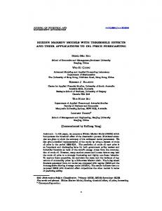
Figure 1: Different levels of the waste representation for the German text fragment “. . . 2,5 Mill. Eur. Durch die . . .” depicted as a tree. Nodes of depth 0, 1, and 2 correspond to the levels of sentences, tokens, and segments, respectively. The feature values used by the HMM boundary detector are given below the corresponding segments. Boldface values of “hidden” features on a green background indicate the correct assignment, while gray values on a white background indicate possible but incorrect assignments.

JLCL

68

Tokenization with HMMs function representing the conjunction over all individual features in F as an n-tuple:

^

F

:

S → rng(f1 ) × rng(f2 ) × . . . × rng(fn )

:

x 7→ hf1 (x), f2 (x), . . . , fn (x)i

(1)

Then, the boundary detection HMM can be defined in the usual way (Rabiner, 1989; Manning and Schütze, 1999) as the 5-tuple D = hQ, O, Π, A, Bi, where:




V

1. Q = rng (Fhide ∪ Fsurf \Fnoctx ) is a finite set of model states, where each state q ∈ Q is represented by a 7-tuple of values for the contextual features class, case, length, blanks, bow, bos, and eos;

V




2. O = rng Fsurf is a finite set of possible observations, where each observation is represented by a 5-tuple of values for the surface features class, case, length, blanks, and stop; 3. Π : Q → [0, 1] : q 7→ p(Q1 = q) is a probability distribution over Q representing the model’s initial state probabilities; 4. A : Qk → [0, 1] : hq1 , . . . , qk i 7→ p(Qi = qk |Qi−k+1 = q1 , . . . , Qi−1 = qk−1 ) is a conditional probability distribution over state k-grams representing the model’s state transition probabilities; and 5. B : Q × O → [0, 1] : hq, oi 7→ p(O = o|Q = q) is a probability distribution over observations conditioned on states representing the model’s emission probabilities. i+j Using the shorthand notation V wi  for the string wi wi+1 . . . wi+j , and writing fO (w) for the observable features Fsurf (w) of a given segment w, the model D computes the probability of a segment sequence w1n as the sum of path probabilities over all possible generating state sequences:

p(W = w1n )

=

X

p(W = w1n , Q = q1n )

(2)

n ∈Qn q1

Assuming suitable boundary handling for negative indices, joint path probabilities themselves are computed as: p(W = w1n , Q = q1n )

=

n Y

i−1 p(qi |qi−k+1 )p(wi |qi )

(3)

i=1

Underlying these equations are the following assumptions: p(qi |q1i−1 , w1i−1 )

=

i−1 p(qi |qi−k+1 )

(4)

p(wi |q1i , w1i−1 )

=

p(wi |qi ) = p(Oi = fO (wi )|Qi = qi )

(5)

Equation (4) asserts that state transition probabilities depend on at most the preceding k − 1 states and thus on the contextual features of at most the preceding k − 1 segments.

JLCL 2013 – Band 28 (2)

69

Jurish, Würzner Equation (5) asserts the independence of a segment’s surface features from all but the model’s current state, formally expressing the context-independence of Fnoctx . In the experiments described below, we used scan-segment trigrams (k = 3) extracted from a training corpus to define language-specific boundary detection models in a supervised manner. To account for unseen trigrams, the empirical distributions were smoothed by linear interpolation of uni-, bi-, and trigrams (Jelinek and Mercer, 1980), using the method described by Brants (2000) to estimate the interpolation coefficients. 2.2.3 Runtime Boundary Placement Having defined the disambiguator model D, it can be used to predict the “best” possible boundary placement for an input sequence of scanner segments W by application of the well-known Viterbi algorithm (Viterbi, 1967). Formally, the Viterbi algorithm computes the state path with maximal probability for the observed input sequence: Viterbi(W, D) =

arg max

p(q1 , . . . , qn , W |D)

(6)

hq1 ,...,qn i∈Qn

If hq1 , . . . , qn i = Viterbi(W, D) is the optimal state sequence returned by the Viterbi algorithm for the input sequence W , the final segmentation into word-like tokens is defined by placing a word boundary immediately preceding all and only those segments wi with i = 1 or qi [bow] = +. Similarly, sentence boundaries are placed before all and only those segments wi with i = 1 or qi [bow] = qi [bos] = qi−1 [eos] = +. Informally, this means that every input sequence will begin a new word and a new sentence, every sentence boundary must also be a word boundary, and a high-level agreement heuristic is enforced between adjacent eos and bos features.6 Since all surface feature values are uniquely determined by observed segment and only the hidden segment features bow, bos, and eos are ambiguous, only those states qi need to be considered for a segment wi which agree with respect to surface features, which represents a considerable efficiency gain, since the Viterbi algorithm’s running time grows exponentially with the number of states considered per observation. 3 Experiments In this section, we present four experiments designed to test the efficacy of the waste boundary detection framework described above. After describing the corpora and software used for the experiments in Section 3.1 and formally defining our evaluation criteria in Section 3.2, we first compare the performance of our approach to that of the Punkt system introduced by Kiss and Strunk (2006) on corpora from five different European languages in Section 3.3. In Section 3.4 we investigate the effect of training corpus size on HMM-based boundary detection, while Section 3.5 deals with the effect 6

Although either of the eos or bos features on its own is sufficient to define a boundary placement model, preliminary experiments showed substantially improved precision for the model presented above using both eos and bos features together with an externally enforced agreement heuristic.

70

JLCL

Tokenization with HMMs Corpus cz de en fr it chat

Sentences 21,656 50,468 49,208 21,562 2,860 11,416

Words 487,767 887,369 1,173,766 629,810 75,329 95,102

Segments 495,832 936,785 1,294,344 679,375 77,687 105,297

Table 3: Corpora used for tokenizer training and evaluation.

of some common typographical conventions. Finally, Section 3.6 describes some variants of the basic waste model and their respective performance with respect to a small corpus of computer-mediated communication. 3.1 Materials Corpora We used several freely available corpora from different languages for training and testing. Since they were used to provide ground-truth boundary placements for evaluation purposes, we required that all corpora provide both word- and sentencelevel segmentation. For English (en), we used the Wall Street Journal texts from the Penn Treebank (Marcus et al., 1993) as distributed with the Prague Czech-English Dependency Treebank (Cuřín et al., 2004), while the corresponding Czech translations served as the test corpus for Czech (cz). The TIGER treebank (de; Brants et al., 2002) was used for our experiments on German.7 French data were taken from the ‘French Treebank’ (fr) described by Abeillé et al. (2003), which also contains annotations for multi-word expressions which we split into their components.8 For Italian, we chose the Turin University Treebank (it; Bosco et al., 2000). To evaluate the performance of our approach on non-standard orthography, we used a subset of the Dortmund Chat Corpus (chat; Beißwenger and Storrer, 2008). Since pre-segmented data are not available for this corpus, we extracted a sample of the corpus containing chat logs from different scenarios (media, university context, casual chats) and manually inserted token and sentence boundaries. To support the detection of (self-)interrupted sentences, we grouped each user’s posts and ordered them according to their respective timestamps. Table 3 summarizes some basic properties of the corpora used for training and evaluation.

7

Unfortunately, corresponding (non-tokenized) raw text is not included in the TIGER distribution. We therefore semi-automatically de-tokenized the sentences in this corpus: token boundaries were replaced by whitespace except for punctuation-specific heuristics, e.g. no space was inserted before commas or dots, or after opening brackets. Contentious cases such as date expressions, truncations or hyphenated compounds were manually checked and corrected if necessary. 8 Multi-word tokens consisting only of numeric and punctuation subsegments (e.g. “16/9 ” or “3,2 ”) and hyphenated compounds (“Dassault-électronique”) were not split into their component segments, but rather treated as single tokens.

JLCL 2013 – Band 28 (2)

71

Jurish, Würzner Software The waste text segmentation system described in Sec. 2 was implemented in C++ and Perl. The initial prolix segmentation of the input stream into candidate segments was performed by a traditional lex-like scanner generated from a set of 49 hand-written regular expressions by the scanner-generator RE2C (Bumbulis and Cowan, 1993).9 HMM training, smoothing, and runtime Viterbi decoding were performed by the moot part-of-speech tagging suite (Jurish, 2003). Viterbi decoding was executed using the default beam pruning coefficient of one thousand in moot’s “streaming mode,” flushing the accumulated hypothesis space whenever an unambiguous token was encountered in order to minimize memory requirements without unduly endangering the algorithm’s correctness (Lowerre, 1976; Kempe, 1997). To provide a direct comparison with the Punkt system beyond that given by Kiss and Strunk (2006), we used the nltk.tokenize.punkt module distributed with the Python NLTK package. Boundary placements were evaluated with the help of GNU diff (Hunt and McIlroy, 1976; MacKenzie et al., 2002) operating on one-word-per-line “vertical” files. Cross-Validation Except where otherwise noted, waste HMM tokenizers were tested by 10-fold cross-validation to protect against model over-fitting: each test corpus C was partitioned on true sentence boundaries into 10 strictly disjoint subcorpora {ci }1≤i≤10 of approximately equal size, S and for each evaluation subcorpus ci , an HMM trained on the remaining subcorpora j6=i cj was used to predict boundary placements in ci . Finally, the automatically annotated evaluation subcorpora were concatenated and evaluated with respect to the original test corpus C. Since the Punkt system was designed to be trained in an unsupervised fashion from raw untokenized text, no cross-validation was used in the evaluation of Punkt tokenizers. 3.2 Evaluation Measures The tokenization method described above was evaluated with respect to the groundtruth test corpora in terms of precision, recall, and the harmonic precision-recall average F, as well as an intuitive scalar error rate. Formally, for a given corpus and a set Brelevant of boundaries (e.g. token- or sentence-boundaries) within that corpus, let Bretrieved be the set of boundaries of the same type predicted by the tokenization procedure to be evaluated. Tokenizer precision (pr) and recall (rc) can then be defined as: pr

=

rc

=

|Brelevant ∩ Bretrieved | tp = tp + fp |Bretrieved | |Brelevant ∩ Bretrieved | tp = tp + fn |Brelevant |

(7) (8)

where following the usual conventions tp = |Brelevant ∩Bretrieved | represents the number of true positive boundaries predicted by the tokenizer, fp = |Bretrieved \Brelevant | represents 9

Of these, 31 were dedicated to the recognition of special complex token types such as URLs and e-mail addresses.

72

JLCL

Tokenization with HMMs the number of false positives, and fn = |Brelevant \Bretrieved | represents the number of false negatives. Precision thus reflects the likelihood of a true boundary given its prediction by the tokenizer, while recall reflects the likelihood that that a boundary will in fact be predicted given its presence in the corpus. In addition to these measures, it is often useful to refer to a single scalar value on the basis of which to compare tokenization quality. The unweighted harmonic precision-recall average F (van Rijsbergen, 1979) is often used for this purpose: F

=

2 × pr × rc pr + rc

(9)

In the sequel, we will also report tokenization error rates (Err) as the ratio of errors to all predicted or true boundaries:10 Err

=

|Brelevant 4Bretrieved | fp + fn = tp + fp + fn |Brelevant ∪ Bretrieved |

(10)

To allow direct comparison with the results reported for the Punkt system by Kiss and Strunk (2006), we will also employ the scalar measure used there, which we refer to here as the “Kiss-Strunk error rate” (ErrKS ): ErrKS

=

fp + fn number of all candidates

(11)

Since the Kiss-Strunk error rate only applies to sentence boundaries indicated by a preceding full stop, we assume that the “number of candidates” referred to in the denominator is simply the number of dot-final tokens in the corpus. 3.3 Experiment 1: WASTE versus Punkt We compared the performance of the HMM-based waste tokenization architecture described in Sec. 2 to that of the Punkt tokenizer described by Kiss and Strunk (2006) on each of the five conventional corpora from Table 3, evaluating the tokenizers with respect to both sentence- and word-boundary prediction. 3.3.1 Sentence Boundaries Since Punkt is first and foremost a disambiguator for sentence boundaries indicated by a preceding full stop, we will first consider the models’ performance on these, as given in Table 4. For all tested languages, the Punkt system achieved a higher recall on dot-terminated sentence boundaries, representing an average relative recall error reduction rate of 54.3% with respect to the waste tokenizer. Waste exhibited greater precision however, providing an average relative precision error reduction rate of 73.9% with respect to Punkt. The HMM-based waste technique incurred the fewest errors 10

A4B represents the symmetric difference between sets A and B: A4B = (A\B) ∪ (B\A).

JLCL 2013 – Band 28 (2)

73

Jurish, Würzner Corpus cz de en fr it

Method waste punkt waste punkt waste punkt waste punkt waste punkt

tp 20,808 19,892 40,887 41,068 47,309 46,942 19,944 19,984 2,437 2,595

fp 158 1,019 128 399 151 632 66 128 15 233

fn 143 46 420 292 109 77 203 112 169 0

pr% 99.25 95.13 99.69 99.04 99.68 98.67 99.67 99.36 99.39 91.76

rc% 99.32 99.77 98.98 99.29 99.77 99.84 98.99 99.44 93.51 100.00

F% 99.28 97.39 99.33 99.17 99.73 99.25 99.33 99.40 96.36 95.70

ErrKS % 1.20 4.52 1.23 1.56 0.40 1.09 1.24 1.10 6.02 7.64

Table 4: Performance on dot-terminated sentences, evaluation following Kiss and Strunk (2006). Corpus cz de en fr it

Method waste punkt waste punkt waste punkt waste punkt waste punkt

tp 21,230 20,126 47,453 41,907 48,162 47,431 20,965 20,744 2,658 2,635

fp 242 1,100 965 497 452 724 143 230 16 240

fn 425 1,529 3,014 8,560 1,045 1,776 596 817 201 223

pr% 98.87 94.82 98.01 98.83 99.07 98.50 99.32 98.90 99.40 91.65

rc% 98.04 92.94 94.03 83.04 97.88 96.39 97.24 96.21 92.97 92.20

F% 98.45 93.87 95.98 90.25 98.47 97.43 98.27 97.54 96.08 91.92

Err% 3.05 11.55 7.74 17.77 3.01 5.01 3.40 4.80 7.55 14.95

Table 5: Overall performance on sentence boundary detection.

overall, and those errors which it did make were more uniformly distributed between false positives and false negatives, leading to higher F values and lower Kiss-Strunk error rates for all tested corpora except French. It is worth noting that the error rates we observed for the Punkt system as reported in Table 4 differ from those reported in Kiss and Strunk (2006). In most cases, these differences can be attributed to the use of different corpora. The most directly comparable values are assumedly those for English, which in both cases were computed based on samples from the Wall Street Journal corpus: here, we observed a similar error rate (1.10%) to that reported by Kiss and Strunk (1.65%), although Kiss and Strunk observed fewer false positives than we did. These differences may stem in part from incompatible criteria regarding precisely which dots can legitimately be regarded as sentence-terminal, since Kiss and Strunk provide no formal definition of what exactly constitutes a “candidate” for the computation of Eq. (11). In particular, it is unclear how sentence-terminating full stops which are not themselves in sentence-final position – as often occurring in direct quotations (e.g. “He said ‘stop.’”) – are to be treated. Despite its excellent recall for dot-terminated sentences, the Punkt system’s performance dropped dramatically when considering all sentence boundaries (Table 5), including those terminated e.g. by question marks, exclamation points, colons, semi-

74

JLCL

Tokenization with HMMs Corpus cz de en fr it

Method waste punkt waste punkt waste punkt waste punkt waste punkt

tp 487,560 463,774 886,937 882,161 1,164,020 1,154,485 625,554 589,988 74,532 71,028

fp 94 10,445 533 9,082 9,228 22,311 2,587 61,236 132 3,514

fn 206 23,993 431 5,208 9,745 19,281 4,255 39,822 796 4,302

pr% 99.98 97.80 99.94 98.98 99.21 98.10 99.59 90.60 99.82 95.29

rc% 99.96 95.08 99.95 99.41 99.17 98.36 99.32 93.68 98.94 94.29

F% 99.97 96.42 99.95 99.20 99.19 98.23 99.46 92.11 99.38 94.78

Err% 0.06 6.91 0.11 1.59 1.60 3.48 1.08 14.62 1.23 9.91

Table 6: Overall performance on word-boundary detection.

colons, or non-punctuation characters. Our approach outperformed Punkt on global sentence boundary detection for all languages and evaluation modes except precision on the German TIGER corpus (98.01% for the waste tokenizer vs. 98.83% for Punkt). Overall, waste incurred only about half as many sentence boundary detection errors as Punkt (µ = 49.3%, σ = 15.3%). This is relatively unsurprising, since Punkt’s rule-based scanner stage is responsible for detecting any sentence boundary not introduced by a full stop, while waste can make use of token context even in the absence of a dot character. 3.3.2 Word Boundaries The differences between our approach and that of Kiss and Strunk become even more apparent for word boundaries. As the data from Table 6 show, waste substantially outperformed Punkt on word boundary detection for all languages and all evaluation modes, reducing the number of word-boundary errors by over 85% on average (µ = 85.6%, σ = 16.0%). Once again, this behavior can be explained by Punkt’s reliance on strict rule-based heuristics to predict all token boundaries except those involving a dot on the one hand, and waste’s deferral of all final decisions to the model-dependent runtime decoding stage on the other. In this manner, our approach is able to adequately account for both “prolix” target tokenizations such as that given by the Czech corpus – which represents e.g. adjacent single quote characters (“) as separate tokens – as well as “terse” tokenizations such as that of the English corpus, which conflates e.g. genitive apostrophe-s markers (’s) into single tokens. While it is almost certainly true that better results for Punkt than those presented in Table 6 could be attained by using additional language-specific heuristics for tokenization, we consider it to be a major advantage of our approach that it does not require such fine-tuning, but rather is able to learn the “correct” word-level tokenization from appropriate training data. Although the Punkt system was not intended to be an all-purpose word-boundary detector, it was specifically designed to make reliable decisions regarding the status of word boundaries involving the dot character, in particular abbreviations (e.g. “etc.”,

JLCL 2013 – Band 28 (2)

75

Jurish, Würzner Corpus cz de en fr it

Method waste punkt waste punkt waste punkt waste punkt waste punkt

tp 0 0 3,048 2,737 16,552 15,819 1,344 1,315 182 153

fp 0 2,658 58 23 521 1,142 30 60 11 76

fn 0 0 101 412 145 878 68 97 12 41

pr% – 0.00 98.13 99.17 96.95 93.27 97.82 95.64 94.30 66.81

rc% – – 96.79 86.92 99.13 94.74 95.18 93.13 93.81 78.87

F% – – 97.46 92.64 98.03 94.00 96.48 94.37 94.06 72.34

Err% – 100.00 4.96 13.71 3.87 11.32 6.80 10.67 11.22 43.33

Table 7: Performance on word boundary detection for dot-final words.

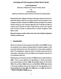
“Inc.”) and ordinals (“24.”). Restricting the evaluation to dot-terminated words containing at least one non-punctuation character produces the data in Table 7. Here again, waste substantially outperformed Punkt for all languages11 and all evaluation modes except for precision on the German corpus (98.13% for waste vs. 99.17% for Punkt), incurring on average 62.1% fewer errors than Punkt (σ = 15.5%). 3.4 Experiment 2: Training Corpus Size It was mentioned above that our approach relies on supervised training from a presegmented corpus to estimate the model parameters used for runtime boundary placement prediction. Especially in light of the relatively high error-rates observed for the smallest test corpus (Italian), this requirement raises the question of how much training material is in fact necessary to ensure adequate runtime performance of our model. To address such concerns, we varied the amount of training data used to estimate the HMM’s parameters between 10,000 and 100,000 tokens,12 using cross-validation to compute averages for each training-size condition. Results for this experiment are given in Figure 2. All tested languages showed a typical logarithmic learning curve for both sentenceand word-boundary detection, and word-boundaries were learned more quickly than sentence boundaries in all cases. This should come as no surprise, since any nontrivial corpus will contain more word boundaries than sentence boundaries, and thus provide more training data for detection of the former. Sentence boundaries were hardest to detect in the German corpus, which is assumedly due to the relatively high frequency of punctuation-free sentence boundaries in the TIGER corpus, in which over 10% of the sentence boundaries were not immediately preceded by a punctuation 11

We ignore the Czech data for the analysis of dot-final word boundaries, since the source corpus included token boundaries before every word-terminating dot character, even for “obvious” abbreviations like “Ms.” and “Inc.” or initials such as in “[John] D. [Rockefeller]”. 12 Training sizes for Italian varied between 7,000 and 70,000 due to the limited number of tokens available in that corpus as a whole.

76

JLCL

Tokenization with HMMs Case + + − −

Punct + − + −

tp 47,453 33,597 44,205 4,814

fp 965 1,749 1,185 3,277

fn 3,014 16,862 6,262 45,645

pr% 98.01 95.05 97.39 59.50

rc% 94.03 66.58 87.59 9.54

F% 95.98 78.31 92.23 16.44

Err% 7.74 35.65 14.42 91.04

Table 8: Effect of typographical conventions on sentence detection for the TIGER corpus (de).

character,13 vs. only 1% on average for the other corpora (σ = 0.78%). English and French were the most difficult corpora in terms of word boundary detection, most likely due to apostrophe-related phenomena including the English genitive marker ’s and the contracted French article l’.

3.5 Experiment 3: Typographical Conventions Despite the lack of typographical clues, the waste tokenizer was able to successfully detect over 3300 of the unpunctuated sentence boundaries in the German TIGER corpus (pr = 94.1%, rc = 60.8%). While there is certainly room for improvement, the fact that such a simple model can perform so well in the absence of explicit sentence boundary markers is encouraging, especially in light of our intent to detect sentence boundaries in non-standard computer-mediated communication text, in which typographical markers are also frequently omitted. In order to get a clearer idea of the effect of typographical conventions on sentence boundary detection, we compared the waste tokenizer’s performance on the German TIGER corpus with and without both punctuation (±Punct) and letter-case (±Case), using cross-validation to train and test on appropriate data, with the results given in Table 8. As hypothesized, both letter-case and punctuation provide useful information for sentence boundary detection: the model performed best for the original corpus retaining all punctuation and letter-case distinctions. Also unsurprisingly, punctuation was a more useful feature than letter-case for German sentence boundary detection,14 the [−Case, +Punct] variant achieving a harmonic precision-recall average of F = 92.23%. Even letter-case distinctions with no punctuation at all sufficed to identify about two thirds of the sentence boundaries with over 95% precision, however: this modest success is attributable primarily to the observations’ stop features, since upper-cased sentenceinitial stopwords are quite frequent and almost always indicate a preceding sentence boundary. 13 14

Most of these boundaries appear to have been placed between article headlines and body text for the underlying newspaper data. In German, not only sentence-initial words and proper names, but also all common nouns are capitalized, so letter-case is not as reliable a clue to sentence boundary placement as it might be for English, which does not capitalize common nouns.

JLCL 2013 – Band 28 (2)

77

Jurish, Würzner

0.18

cz de en fr it

0.16

Error Rate (s)

0.14

0.12

0.1

0.08

0.06

0.04 10000

20000

30000

40000 50000 60000 70000 Number of Training Tokens

80000

0.03

90000

100000

cz de en fr it

0.025

Error Rate (w)

0.02

0.015

0.01

0.005

0 10000

20000

30000

40000 50000 60000 70000 Number of Training Tokens

80000

90000

100000

Figure 2: Effect of training corpus size on sentence boundary detection (top) and word boundary detection (bottom).

78

JLCL

Tokenization with HMMs Model chat chat[+force] chat[+feat] tiger tiger[+force]

tp 7,052 11,088 10,524 2,537 10,396

fp 1,174 1,992 784 312 1,229

fn 4,363 327 891 8,878 1,019

pr% 85.73 84.77 93.07 89.05 89.43

rc% 61.78 97.14 92.19 22.23 91.07

F% 71.81 90.53 92.63 35.57 90.24

Err% 43.98 17.30 13.73 78.37 17.78

Table 9: Effect of training source on sentence boundary detection for the chat corpus.

3.6 Experiment 4: Chat Tokenization We now turn our attention to the task of segmenting a corpus of computer-mediated communication, namely the chat corpus subset described in Sec. 3.1. Unlike the newspaper corpora used in the previous experiments, chat data is characterized by non-standard use of letter-case and punctuation: almost 37% of the sentences in the chat corpus were not terminated by a punctuation character, and almost 70% were not introduced by an upper-case letter. The chat data were subdivided into 10, 289 distinct observable utterance-like units we refer to as posts; of these, 9479 (92.1%) coincided with sentence boundaries, accounting for 83% of the sentence boundaries in the whole chat corpus. We measured the performance of the following five distinct waste tokenizer models on sentence- and word-boundary detection for the chat corpus: • chat: the standard model as described in Section 2, trained on a disjoint subset of the chat corpus and evaluated by cross-validation; • chat[+force]: the standard model with a supplemental heuristic forcing insertion of a sentence boundary at every post boundary; • chat[+feat]: an extended model using all features described in Section 2.2.1 together with additional binary contextual surface features bou and eou encoding whether or not the corresponding segment occurs at the beginning or end of an individual post, respectively; • tiger: the standard model trained on the entire TIGER newspaper corpus; and • tiger[+force]: the standard tiger model with the supplemental [+force] heuristic for sentence boundary insertion at every post boundary. Results for chat corpus sentence boundary detection are given in Table 9 and for word boundaries in Table 10. From these data, it is immediately clear that the standard model trained on conventional newspaper text (tiger) does not provide a satisfactory segmentation of the chat data on its own, incurring almost twice as many errors as the standard model trained by cross-validation on chat data (chat). This supports our claim that chat data represent unconventional and non-standard uses of modelrelevant features, in particular punctuation and capitalization. Otherwise, differences between the various cross-validation conditions chat, chat[+force], and chat[+feat] with respect to word-boundary placement were minimal.

JLCL 2013 – Band 28 (2)

79

Jurish, Würzner Model chat chat[+force] chat[+feat] tiger tiger[+force]

tp 93,167 93,216 93,235 91,603 91,611

fp 1,656 1,612 1,595 5,889 5,971

fn 1,934 1,885 1,866 3,499 3,491

pr% 98.25 98.30 98.32 93.96 93.88

rc% 97.97 98.02 98.04 96.32 96.33

F% 98.11 98.16 98.18 95.13 95.09

Err% 3.71 3.62 3.58 9.30 9.36

Table 10: Effect of training source on word boundary detection for the chat corpus.

Sentence-boundary detection performance for the standard model (chat) was similar to that observed in Section 3.5 for newspaper text with letter-case but without punctuation, EOS recall in particular remaining unsatisfactory at under 62%. Use of the supplemental [+force] heuristic to predict sentence boundaries at all post boundaries raised recall for the newspaper model (tiger[+force]) to over 91%, and for the crossvalidation model (chat[+force]) to over 97%. The most balanced performance however was displayed by the extended model chat[+feat] using surface features to represent the presence of post boundaries: although its error rate was still quite high at almost 14%, the small size of the training subset compared to those used for the newspaper corpora in Section 3.3 leaves some hope for improvement as more training data become available, given the typical learning curves from Figure 2. 4 Conclusion We have presented a new method for estimating sentence and word token boundaries in running text by coupling a prolix rule-based scanner stage with a Hidden Markov Model over scan-segment feature bundles using hidden binary features bow, bos, and eos to represent the presence or absence of the corresponding boundaries. Language-specific features were limited to an optional set of user-specified stopwords, while the remaining observable surface features were used to represent basic typographical class, letter-case, word length, and leading whitespace. We compared our “waste” approach to the high-quality sentence boundary detector Punkt described by Kiss and Strunk (2006) on newspaper corpora from five different European languages, and found that the waste system not only substantially outperformed Punkt for all languages in detection of both sentence- and word-boundaries, but even outdid Punkt on its “home ground” of dot-terminated words and sentences, providing average relative error reduction rates of 62% and 33%, respectively. Our technique exhibited a typical logarithmic learning curve, and was shown to adapt fairly well to varying typographical conventions given appropriate training data. A small corpus of computer-mediated communication extracted from the Dortmund Chat Corpus (Beißwenger and Storrer, 2008) and manually segmented was introduced and shown to violate some typographical conventions commonly used for sentence boundary detection. Although the unmodified waste boundary detector did not perform as well as hoped on these data, the inclusion of additional surface features

80

JLCL

Tokenization with HMMs sensitive to observable post boundaries sufficed to achieve a harmonic precision-recall average F of over 92%, representing a relative error reduction rate of over 82% with respect to the standard model trained on newspaper text, and a relative error reduction rate of over 38% with respect to a naïve domain-specific splitting strategy. Acknowledgements Research was supported by the Deutsche Forschungsgemeinschaft grants KL 337/12-2 and KL 955/19-1. We are grateful to Sophie Arana, Maria Ermakova, and Gabriella Pein for their help in manual preparation of the chat corpus used in section 3.6. The waste system described above is included with the open-source moot package, and can be tested online at http://www.dwds.de/waste/. Finally, we would like to thank this article’s anonymous reviewers for their helpful comments. References Abeillé, A., Clément, L., and Toussenel, F. (2003). Building a treebank for French. In Abeillé, A., editor, Treebanks, volume 20 of Text, Speech and Language Technology, pages 165–187. Springer. Beißwenger, M. and Storrer, A. (2008). Corpora of Computer-Mediated Communication. In Lüdeling, A. and Kytö, M., editors, Corpus Linguistics. An International Handbook, pages 292–308. De Gruyter. Bird, S., Klein, E., and Loper, E. (2009). Natural Language Processing with Python. O’Reilly, Sebastopol, CA. Bosco, C., Lombardo, V., Vassallo, D., and Lesmo, L. (2000). Building a treebank for Italian: a data-driven annotation schema. In Proceedings LREC ’00, Athens, Greece. Brants, S., Dipper, S., Hansen, S., Lezius, W., and Smith, G. (2002). The TIGER treebank. In Proceedings of the Workshop on Treebanks and Linguistic Theories, Sozopol. Brants, T. (2000). TnT – a statistical part-of-speech tagger. In Proceedings of the Sixth Applied Natural Language Processing Conference ANLP-2000, Seattle, WA. Bumbulis, P. and Cowan, D. D. (1993). RE2C: a more versatile scanner generator. ACM Letters on Programming Languages and Systems, 2(1-4):70–84. Church, K. W. (1988). A stochastic parts program and noun phrase parser for unrestricted text. In Proceedings of the 2nd Conference on Applied Natural Language Processing (ANLP), pages 136–143. Cuřín, J., Čmejrek, M., Havelka, J., Hajič, J., Kuboň, V., and Žabokrtsk` y, Z. (2004). Prague Czech-English dependency treebank version 1.0. Linguistic Data Consortium, Catalog No.: LDC2004T25. Francis, W. N. and Kucera, H. (1982). Frequency analysis of English usage: Lexicon and Grammar. Houghton Mifflin.

JLCL 2013 – Band 28 (2)

81

Jurish, Würzner Grefenstette, G. and Tapanainen, P. (1994). What is a word, What is a sentence? Problems of Tokenization. In Proceedings of the 3rd Conference on Computational Lexicography and Text Research, COMPLEX ’94, pages 79–87. He, Y. and Kayaalp, M. (2006). A Comparison of 13 Tokenizers on MEDLINE. Technical Report LHNCBC-TR-2006-03, U.S. National Library of Medicine. Hunt, J. W. and McIlroy, M. D. (1976). An algorithm for differential file comparison. Computing Science Technical Report 41, Bell Laboratories. Jelinek, F. and Mercer, R. L. (1980). Interpolated estimation of Markov source parameters from sparse data. In Gelsema, E. S. and Kanal, L. N., editors, Pattern Recognition in Practice, pages 381–397. North-Holland Publishing Company, Amsterdam. Jurish, B. (2003). A hybrid approach to part-of-speech tagging. Technical report, Project “Kollokationen im Wörterbuch”, Berlin-Brandenburg Academy of Sciences, Berlin. Kempe, A. (1997). Finite state transducers approximating hidden markov models. In Proceedings of the 35th Annual Meeting of the Association for Computational Linguistics, pages 460–467. Kiss, T. and Strunk, J. (2006). Unsupervised multilingual sentence boundary detection. Computational Linguistics, 32(4):485–525. Lowerre, B. T. (1976). The HARPY speech recognition system. PhD thesis, Carnegie Mellon University. MacKenzie, D., Eggert, P., and Stallman, R. (2002). Comparing and Merging Files with GNU diff and patch. Network Theory Ltd., Bristol, UK. Manning, C. D. and Schütze, H. (1999). Foundations of Statistical Natural Language Processing. MIT Press, Cambridge, MA. Marcus, M. P., Santorini, B., Marcinkiewicz, M. A., and Taylor, A. (1993). Building a large annotated corpus of English: the Penn Treebank. Computational Linguistics, 19(2):313–330. Mikheev, A. (2000). Tagging Sentence Boundaries. In Proceedings of the 1st Meeting of the North American Chapter of the Association for Computational Linguistics, pages 264–271. Palmer, D. D. and Hearst, M. A. (1997). Adaptive multilingual sentence boundary disambiguation. Computational Linguistics, 23(2):241–267. Rabiner, L. R. (1989). A tutorial on Hidden Markov Models and selected applications in speech recognition. Proceedings of the IEEE, 77(2):257–286. Riley, M. D. (1989). Some applications of tree-based modelling to speech and language. In Proceedings of the DARPA Speech and Natural Language Workshop, Human Language Technology Workshops ’89, pages 339–352. Schmid, H. (2000). Unsupervised Learning of Period Disambiguation for Tokenisation. Internal report, Institut für Maschinelle Sprachverarbeitung, Universität Stuttgart. Skut, W. and Brants, T. (1998). Chunk tagger - statistical recognition of noun phrases. CoRR, cmp-lg/9807007.

82

JLCL

Tokenization with HMMs Tomanek, K., Wermter, J., and Hahn, U. (2007). Sentence and token splitting based on conditional random fields. In Proceedings of the 10th Conference of the Pacific Association for Computational Linguistics, pages 49–57. Unicode Consortium (2012). The Unicode Standard, Version 6.2.0. The Unicode Consortium, Mountain View, CA. van Rijsbergen, C. J. (1979). Information Retrieval. Butterworth-Heinemann, Newton, MA. Viterbi, A. J. (1967). Error bounds for convolutional codes and an asymptotically optimal decoding algorithm. IEEE Transications on Information Theory, pages 260–269.

JLCL 2013 – Band 28 (2)

83