Work-Conserving Distributed Schedulers for Terabit Routers Prashanth Pappu
Jonathan Turner
Ken Wong
Washington University Washington University Washington University Computer Science and Engineering Computer Science and Engineering Computer Science and Engineering St. Louis, MO 63130-4899 St. Louis, MO 63130-4899 St. Louis, MO 63130-4899 +1-314-935-4306 +1-314-935-8552 +1-314-935-7524
[email protected]
[email protected]
ABSTRACT − Buffered multistage interconnection networks offer one of the most scalable and cost-effective approaches to building high capacity routers. Unfortunately, the performance of such systems has been difficult to predict in the presence of the extreme traffic conditions that can arise in the Internet. Recent work introduced distributed scheduling, to regulate the flow of traffic in such systems. This work demonstrated, using simulation and experimental measurements, that distributed scheduling can deliver robust performance for extreme traffic. Here, we show that distributed schedulers can be provably work-conserving for speedups of 2 or more. Two of the three schedulers we describe were inspired by previously published crossbar schedulers. The third has no direct counterpart in crossbar scheduling. In our analysis, we show that distributed schedulers based on blocking flows in small-depth acyclic flow graphs can be work-conserving, just as certain crossbar schedulers based on maximal bipartite matchings have been shown to be work-conserving. We also study the performance of practical variants of these schedulers when the speedup is less than 2, using simulation. Categories and Subject Descriptors. C.2.1 [ComputerCommunications Networks]: Network Architecture and Design – network communications, packet-switching networks. General Terms. algorithms, performance Keywords. distributed scheduling, crossbar scheduling, performance routers, CIOQ switches
high
1. INTRODUCTION High performance routers must be scalable to hundreds or even thousands of ports. The most scalable router architectures include systems using multistage interconnection networks with internal buffers and a small speedup relative to the external links; that is, the internal data paths operate at speeds that are greater than the
This work supported by DARPA (contract #N660001-01-1-8930) and NSF (ANI-0325298). Permission to make digital or hard copies of all or part of this work for personal or classroom use is granted without fee provided that copies are not made or distributed for profit or commercial advantage and that copies bear this notice and the full citation on the first page. To copy otherwise, or republish, to post on servers or to redistribute to lists, requires prior specific permission and/or a fee. SIGCOMM’04, Aug. 30–Sept. 3, 2004, Portland, Oregon, USA. Copyright 2004 ACM 1-58113-862-8/04/0008...$5.00.
[email protected]
external links by a small constant factor (typically between 1 and 2). In the presence of a sustained overload at an output port, such systems can become congested with traffic attempting to reach the overloaded output, interfering with the flow of traffic to other outputs. The unregulated nature of traffic in IP networks makes such overloads a normal fact of life, which router designers must address, in order to make their systems robust. Reference [11] introduced distributed scheduling to manage the flow of traffic through a large router in order to mitigate the worst effects of extreme traffic. Distributed scheduling borrows ideas developed for scheduling packet transmissions through crossbar switches [2,5,7,8]. The core idea is to use Virtual Output Queues (VOQ) at each input. That is, each input maintains separate queues for each output. (Queues are implemented as linked lists, so the only per queue overhead is for the queues’ head and tail pointers.) Packets arriving at inputs are placed in queues corresponding to their outgoing links. In crossbar scheduling, a centralized scheduler selects packets to send through the crossbar, seeking to emulate as closely as possible, the queueing behavior of an ideal output queued switch. The centralized scheduler used in crossbar scheduling makes scheduling decisions every packet transmission interval. For routers with 10 Gb/s links, this typically means making scheduling decisions every 40 ns, a demanding requirement, even for routers with small numbers of links. For larger routers it makes centralized scheduling infeasible. Distributed scheduling, unlike crossbar scheduling, does not seek to schedule the transmission of individual packets. Instead, it regulates the number of packets forwarded during a period which we call the scheduling interval and denote by T. The scheduling interval is typically fairly long, on the order of tens of microseconds. The use of such coarse-grained scheduling means that a distributed scheduler can only approximate the queueing behavior of an ideal output-queued switch, but does allow systems to scale up to larger configurations than are practical with fine-grained scheduling. In a router that implements distributed scheduling, the Port Processors (the components that terminate the external links, make routing decisions and queue packets) periodically exchange information about the status of their VOQs. This information is then used to rate control the VOQs, with the objective of moving packets to the output side of the router as expeditiously as possible, while avoiding congestion within the interconnection network. So long as the scheduling interval is kept small relative to end-to-end delays (which are typically tens to hundreds of milli-
seconds in wide area networks) the impact of coarse scheduling on the delays experienced by packets can be acceptably small. While [11] demonstrated, using simulation and experimental measurement, that distributed scheduling can deliver excellent performance under extreme traffic conditions, it provided no analytical bounds on the performance of the proposed algorithms, nor a rigorous justification for the specific design choices. This paper corrects that deficiency, by showing that there are distributed schedulers that are provably work-conserving, for speedups of 2 or more. The analysis provides insight that motivates the design of more practical variants of these algorithms, which provide excellent performance (significantly better than reported in [11]). Where the algorithms described in [11] can fail to be workconserving, with speedups of more than 2, the algorithms reported here are demonstrably work-conserving for extreme traffic, even when speedups are less than 2. One interesting aspect of the analysis is the role played by network flows, which parallels the role played by bipartite matching in crossbar scheduling. Specifically, distributed schedulers that are based on finding blocking flows in small depth acyclic flow graphs and that favor outputs with short queues are work-conserving, much as crossbar schedulers based on finding maximal matchings in bipartite graphs that favor outputs with short queues are work-conserving. Before proceeding further, it’s important to define what we mean by work-conserving. A crossbar scheduler is workconserving if, in a system using that scheduler, an output link can be idle only if there is no packet in the system for that output. Work-conserving systems match the throughput of ideal output queueing switches, under all possible traffic conditions. In the context of distributed scheduling, the definition of workconservation must be relaxed to reflect the use of coarse-grained scheduling. In section 2, we adopt an idealized definition of workconservation for the purposes of analysis. We discuss the practical implications of this in section 6. It should be noted that while the practical distributed scheduling algorithms discussed here are not work-conserving, practical crossbar scheduling algorithms are also not work-conserving, even though it has been known for several years that there are work-conserving crossbar scheduling algorithms that are too complex to use in real systems. The contribution of this work is to show that distributed scheduling for buffered multistage networks can provide similar performance to what was previously known for crossbar schedulers. While distributed scheduling shares some features of crossbar scheduling, it differs in two important respects. First, the distributed nature of these methods rules out the use of the iterative matching methods that have proved effective in crossbar scheduling, since each iteration would require an exchange of information, causing the overhead of the algorithm to increase in proportion to the number of iterations. On the other hand, the coarsegrained nature of distributed scheduling provides some flexibility that is not present in crossbar scheduling, where it is necessary to match inputs and outputs in a one-to-one fashion during each scheduling operation. In distributed scheduling, we allocate the interface bandwidth at each input and output and may subdivide that bandwidth in whatever proportions produce the best result. Recently, there has been considerable interest in a switch architecture called the load balanced switch described in [4] and used in [6]. This architecture consists of a single stage of buffers
sandwiched between two identical stages of switching, each of which walks through a fixed sequence of configurations. The fixed sequence of switch configurations makes the switching components very simple and the system is capable of achieving 100% throughput for random traffic. Unfortunately, this architecture also has a significant drawback. To avoid resequencing errors, each output requires a resequencing buffer capable of holding about n2 packets. These buffers impose a delay that grows as the square of the switch size. For the 600 port switch described in [6], operated with a switching period of 100 ns, this translates to a delay of about 36 milliseconds, a penalty which applies to all packets, not just to an occasional packet. This appears to be an intrinsic characteristic of the load balancing architecture, and one that significantly limits its attractiveness. Section 2 introduces two scheduling methods, proves that schedulers based on these methods are work-conserving when the speedup is at least 2 and shows how they can be implemented. Section 3 shows how one can implement a practical distributed scheduler, based on one of these methods and evaluates its performance for speedups less than 2, using simulation. Section 4 introduces a more sophisticated, scheduling method, shows that it too is work-conserving when the speedup is at least 2 and shows how it can be implemented using minimum cost blocking flows in networks with convex cost functions. Section 5 describes a practical variant of this method and evaluates it using simulation, showing that it can out-perform the simpler schedulers studied earlier. Section 6 discusses several important practical considerations for distributed scheduling.
2. WORK-CONSERVING SCHEDULERS We describe a general scheduling strategy that can be used to obtain work-conserving schedulers for speedups of 2 or more. While these algorithms are not practical, they provide a conceptual foundation for other algorithms that are. For the purposes of analysis, we adopt an idealized view of the system operation. Specifically, we assume that the system operates in three discrete phases: an arrival phase, a transfer phase and a departure phase. During the arrival phase, each input receives up to T cells.1 During the transfer phase, cells are moved from inputs to outputs, with each input constrained to send at most ST cells (S being the speedup of the system) and each output constrained to receive at most ST. During the output phase, each output forwards up to T cells. A scheduler determines which cells are transferred during the transfer phase. We say that a scheduler is work-conserving if during every departure phase, all outputs for which some input has cells at the start of the departure phase, transmit T cells during the departure phase. The scheduling methods that we study in this section maintain an ordering of the non-empty VOQs at each input. The ordering of the VOQs can be extended to all the cells at an input. Two cells in the same VOQ are ordered according to their position in the VOQ. Cells in different VOQs are ordered according the VOQ ordering. We say that a cell b precedes a cell c at the same input, if b comes before c in this ordering. For any cell c at an input, we let p(c) be
1.
We assume throughout, that variable-length packets are segmented into fixed-length units for transmission through the interconnection network. We refer to these units as cells.
the number of cells at the same input as c that precede c and we let q(c) be the number of cells at the output that c is going to.
from one time step to the next, so slack(c) remains ≥−T at the end of each subsequent arrival phase, while c remains at the input.
We refer to a cell c as an ij-cell if it is at input i and is destined for output j. We say that a scheduling algorithm is maximal if during any transfer phase in which there is an ij-cell c that remains at input i, either input i transfers ST cells or output j receives ST cells. Given a method for ordering the cells at each input, we say that a scheduler is ordered, if in any transfer phase in which an ij-cell c remains at input i, either input i transfers ST cells that precede c or output j receives ST cells. Our scheduling methods produce schedules that are maximal and ordered. We can vary the method by using different VOQ orderings. We describe two ordering methods that lead to work-conserving schedulers.
If a cell c arrives during step t and its VOQ is empty when it arrives, then the rule used to order the VOQ relative to the others ensures that slack(c) ≥ 0 right after it arrives. Hence, slack(c) ≥ −T at the end of the arrival phase and this remains true at the end of each subsequent arrival phase, so long as c remains at the input.
For any cell c waiting at an input, we define the quantity slack(c) = q(c) − p(c). For each of the methods studied, we’ll show that slack(c) ≥ T at the start of each departure phase if S ≥ 2. This implies that for any output with fewer than T cells in its outgoing queue, there can be no cells waiting in any input-side VOQs. This implies that the scheduler is work-conserving.
2.1 Batch Critical Cells First Our first scheduling method is based on ideas first developed in the Critical Cells First scheduler of [5]. Hence, we refer to it as the Batch Critical Cells First (BCCF) method. In BCCF, the relative ordering of two VOQs remains the same so long as they remain non-empty, but when a new VOQ becomes non-empty, it must be ordered relative to the others. When a cell c arrives and the VOQ for c’s output is empty, we insert the VOQ into the existing ordering based on the magnitude of q(c). In particular, if the ordered list of VOQs is v1, v2, . . . , we place the VOQ immediately after the queue vj determined by the largest integer j for which the number of cells in the combined queues v1, . . . ,vj is no larger than q(c). This ensures that slack(c) is non-negative right after c arrives. A specific scheduler is an instance of the BCCF method if it produces schedules that are maximal and ordered with respect to this VOQ ordering method. To show that slack(c) ≥ T at the start of each departure phase, we need two lemmas. Lemma 1. For any BCCF scheduler, if c is any cell that remains at its input during a transfer phase, then slack(c) increases by at least ST during the transfer phase. proof. Since the VOQ ordering does not change during a transfer phase (more precisely, VOQs that remain non-empty retain the same relative order), any maximal, ordered scheduling algorithm either causes q(c) to increase by ST or causes p(c) to decrease by ST. In either case, slack(c) increases by ST. Note that as long as a cell c remains at an input, each arrival phase and departure phase cause slack(c) to decrease by at most T. So, if S ≥2, slack(c) cannot decrease over the course of a complete time step.
If a cell c arrives during step t and its VOQ is not empty, but was empty at the start of the arrival phase, then let b be the first arriving cell to be placed in c’s VOQ during this arrival phase. Then, slack(b) was at least 0 at the time it arrived and at most T−1 cells could have arrived after b did in this arrival phase. If exactly r of these precede b, then at the end of the arrival phase,
slack (c) ≥ slack (b) − ((T − 1) − r ) ≥ (− r ) − ((T − 1) − r ) ≥ −T If a cell c arrives during step t and its VOQ was not empty at the start of the arrival phase, then let b be the last cell in c’s VOQ at the start of the arrival phase. By the induction hypothesis, slack(b) ≥ −T at the end of the previous arrival phase. Since the subsequent transfer phase increases slack(b) by at least 2T and the departure phase decreases it by at most T, slack(b) ≥ 0 at the start of the arrival phase in step t. During this arrival phase, at most T new cells arrive at c’s input. Let r be the number of these arriving cells that precede b. Then at the end of the arrival phase
slack (c) ≥ slack (b) − ((T − 1) − r ) ≥ (− r ) − ((T − 1) − r ) ≥ −T Hence, slack(c) ≥ −T at the end of the arrival phase in all cases and this remains true at the end of each subsequent arrival phase, so long as c remains at the input. Lemma 2 leads directly to the following theorem. Theorem 1. For S ≥2, any BCCF scheduler is work-conserving.
2.2 Batch LOOFA Our second scheduling method is based on ideas first developed in the Least Occupied Output First method of [7], so we refer to it as the Batch Least Occupied Output First (BLOOFA) method. In BLOOFA, VOQs are ordered according to the number of cells in their output-side queues. VOQs going to outputs with fewer cells precede VOQs going to outputs with more cells. Outputs with equal numbers of cells are ordered by the numbering of the outputs. We define BLOOFA as the combination of this ordering method with any maximal, ordered scheduler. We show that slack(c) ≥ T at the start of each departure phase, using the same overall strategy used for BCCF. As before, we need two lemmas. The arguments are similar, but are complicated by the fact that the relative ordering of VOQs can change during a transfer phase.
Lemma 2. For any BCCF scheduler with S ≥2, if c is any cell at an input just before the start of a departure phase, slack(c) ≥ T.
Lemma 3. For any BLOOFA scheduler, during a transfer phase, the minimum slack at any input that does not transfer all of its cells during the transfer phase, increases by at least ST.
proof. We show that for any cell c present at the end of an arrival phase, slack(c) ≥ −T. The result then follows from Lemma 1 and the fact that S ≥2. The proof is by induction on the time step.
proof. Let c be any ij-cell at input i. Let minSlack be the smallest value of the slack among the cells at input i just before the transfer phase, and let slack(c) = minSlack + σ. We will show that slack(c) increases by at least ST − σ during the transfer phase. The lemma then follows directly. (Note that it is not sufficient to prove that the slack of a cell c that has minimum slack at the start
For any cell c that arrives during the first time step, p(c) ≤ T at the end of the arrival phase, so slack(c) ≥ −T at the end of the arrival phase. Since S ≥2, there can be no net decrease in slack(c)
of the transfer phase increases by ST, since c may not be a cell of minimum slack at the end of the transfer phase.) We say that a cell b at input i passes c, if before the transfer phase, c precedes b and after the transfer phase b precedes c. If no cells pass c during the transfer phase, then by the definition of maximal, ordered schedulers, either q(c) increases by ST or p(c) decreases by ST. Either way, slack(c) increases by at least ST − σ. Assume then, that there are r >0 cells that pass c and let b be the cell in the set of cells that pass c that comes latest in the cell ordering (before the transfer phase). For clarity, let q0(x) denote the value of q(x) before the transfer phase and let qF(x) denote the value of q(x) after the transfer phase. Similarly for p and slack. Let m be the number of cells received by output j during the transfer and let k be the number of cells that precede b before the transfer, but do not precede c. Then,
q0 (c) + m = q F (c) ≥ q F (b) ≥ q0 (b) and p0(b) = p0(c) + k. Now,
q0 (c) − p0 (c) = minSlack + σ ≤ q0 (b) − p0 (b) + σ ≤ ( q 0 (c ) + m ) − ( p 0 ( c ) + k ) + σ So (m− k) ≥ − σ. Since b passes c, its output must receive fewer than m cells during the transfer phase, so ST cells that precede it at the start of the transfer phase must be forwarded. Of these at least ST− (k−r) must also precede c at the start of the phase. So,
p F (c ) ≤ p 0 (c ) + r − ( ST − ( k − r )) ≤ p 0 (c ) − ST + k Combining this, with qF(c) = q0(c) + m gives,
slack F (c) = q F (c) − p F (c) ≥ (q0 (c) + m) − ( p0 (c) − ST + k ) ≥ slack 0 (c) + ST + (m − k ) ≥ slack 0 (c) + ST − σ That is, slack(c) increases by at least ST − σ. Note that each arrival phase causes slack(c) to decrease by at most T. However, it is not so easy to bound the decrease in slack(c) during a departure phase. The complicating factor is that cells at c’s input can pass it during a departure phase, making it hard to bound the overall change in slack(c). However, if slack(c) is at least T before the departure phase begins, then q(c) must also be at least T. This means that T cells will depart from c’s output, making it impossible for other cells at c’s input to pass c. Thus, if slack(c) is at least T before the departure phase, then slack(c) is at least 0 after the departure phase. It turns out that this is sufficient to establish that BLOOFA is work-conserving when S ≥ 2. Lemma 4. For any BLOOFA scheduler with S ≥ 2, if c is a cell at an input before the start of a departure phase, then slack(c) ≥ T. proof. We show that for any cell c present at the end of the arrival phase, slack(c) ≥ −T. The result then follows from Lemma 3 and the fact that S ≥2. The proof is by induction on the time step. For any cell c that arrives during the first time step, p(c) ≤ T at the end of the arrival phase, so slack(c) ≥ −T at the end of the arrival phase. Since S ≥2, Lemma 3 implies that slack(c) ≥ T at the end of the transfer phase, if it is still present at the input. By the
discussion just before the statement of Lemma 4, this means that slack(c) ≥ 0 following the departure phase, which in turn means that slack(c) ≥ −T at the end of the next arrival phase. This remains true at the end of every subsequent arrival phase until c is transferred to the output. Suppose then, that c arrives during step t. If, at the end of the arrival phase, the only cells that precede c also arrived during step t, then slack(c) ≥ −T at the end of the arrival phase. By the argument at the end of the last paragraph, this remains true at the end of every subsequent arrival phase until c is transferred. If at the end of the arrival phase in step t, there are cells that precede c that were present at the start of the arrival phase, then let b be the cell in this set of cells that does not precede any of the others in the set. Because b arrived before step t, slack(b) ≥ −T at the end of the previous arrival phase, by the induction hypothesis. This implies that slack(b) ≥ 0 at the start of the arrival phase in step t. Let k be the number of cells that arrive during the arrival phase of step t that precede b at the end of the arrival phase. Let m be the number of cells that arrive during the arrival phase that precede c but not b at the end of the arrival phase. Since k + m ≤ T and slack(b) ≥ −k,
slack (c) = q(c) − p(c) ≥ q(b) − ( p(b) + m) = slack (b) − m ≥ −(m + k ) ≥ −T This remains true at the end of each subsequent arrival phase, so long as c remains at the input. Lemma 4 leads directly to the following theorem. Theorem 2. For S ≥2, any BLOOFA scheduler is work-conserving.
2.3 Implementation issues We have shown that the combination of two different VOQ ordering strategies with a maximal, ordered scheduler ensures workconserving operation when the speedup is at least 2. We now need to show how to realize a maximal, ordered scheduler. We start with a centralized algorithm and then show how it can be converted into an iterative, distributed algorithm. While the overhead of such iterative algorithms makes them impractical, they provide the basis for non-iterative algorithms that are practical. The key observation is that the scheduling problem can be reduced to finding a blocking flow in an acyclic flow network [13]. A flow network is a directed graph with a distinguished source vertex s, a distinguished sink vertex t and a non-negative capacity for each edge. A flow, in such a network, is a non-negative function defined on the edges. The flow on an edge must not exceed its capacity and for every vertex but s and t, the sum of the flows on the incoming edges must equal the sum of the flows on the outgoing edges. An edge in the network is called saturated, if its flow is equal to its capacity. A blocking flow is one for which every path from s to t contains at least one saturated edge. (Note that a blocking flow is not necessarily a maximum flow.) To convert the scheduling problem to the problem of finding a blocking flow, we first need to construct a flow network. Our network has a source s, a sink t, n vertices referred to as inputs and another n vertices referred to as outputs. There is an edge with capacity ST from s to each input. Similarly, there is an edge with capacity ST from each output to t. For each non-empty VOQ at input i of the router with cells for output j, there is an edge in the flow network from input i to output j with capacity equal to
inputs
VOQ levels
0
outputs 1
2
3
0
6
0 12 0
1
4
5
2
0
6 14 5
3
5
0
output queue levels
2
0
0 0 3
Blocking Flow Problem with Solution capacity,flow 12,12
6 s
4 5
S = 1.5 T=8
12,12 12,12 12,6
a0 a1 a2
6,6 12,6
b0
4,4
5,5
b1
6,6 5,2
a3
14,6 5,0 4,4
Scheduling Solution
6,3
b2
0
outputs 1
2
3
12,12
0
6
0
6
0
12,11
1
4
5
0
3
2
0
6
6
0
3
2
0
0
4
12,12 12,7
t
inputs
Scheduling Problem
b3
Fig. 1. Example showing a maximal ordered schedule constructed from a blocking flow. the number of cells in the VOQ. (An example of a flow network constructed to solve a particular scheduling problem together with the corresponding solution is shown in Fig. 1.) For any integer-valued flow, we can construct a schedule that transfers cells from input i to output j based on the flow on the edge from input i to output j. Such a schedule does not violate any of the constraints on the number of cells that can be sent from any input or to any output. Also, any blocking flow corresponds to a maximal schedule, since any blocking flow corresponding to a schedule that fails to transfer a cell c from input i to output j cannot saturate the edge from input i to output j; hence it must saturate the edge from s to i or the edge from j to t. Such a flow corresponds to a schedule in which either input i sends ST cells or output j receives ST. Dinic’s algorithm [13] for the maximum flow problem constructs blocking flows in acyclic flow networks as one step in its execution. There are several variants of Dinic’s algorithm, that use different methods of constructing blocking flows. The most straightforward method is to repeatedly search for st-paths with no saturated edges and add as much flow as possible along such paths. We can obtain a maximal, ordered scheduler by modifying Dinic’s algorithm so that it preferentially selects edges between input vertices and output vertices, according to the VOQ ordering at the input. The blocking flow shown in Fig. 1 was constructed in this way, based on the BLOOFA ordering. If paths are found using depth-first search and edges leading to dead-ends are removed, Dinic’s algorithm finds a blocking flow in O(mn) time where m is the number of edges and n is the number of vertices. Because the flow graphs used here have bounded depth and because the number of inputs, outputs and edges are all bounded by the number of non-empty VOQs, the algorithm finds a blocking flow in O(v) time where v is the number of non-empty VOQs. This yields an optimal centralized scheduler. However, since v can be as large as n2 (where n is the number of router ports), this is not altogether practical. We can obtain a distributed, iterative scheduling algorithm based on similar ideas. Rather than state this in the language of blocking flows, we describe it directly as a scheduling algorithm. In the distributed scheduler, we first have an exchange of messages in which each output announces the number of cells in its outgoing queue. The inputs use this information to maintain their VOQ order. Note that this requires that each output send n messages and each input receive n messages. Next, the inputs and outputs proceed through a series of rounds.
In each round, inputs that have uncommitted cells to send and have not yet committed to sending ST cells, send bid messages to those outputs that are still prepared to accept more cells. The inputs construct their bids in accordance with the VOQ ordering. In particular, an input commits all the cells it has for the first output in the ordering and makes similar maximal bids for subsequent outputs until it has placed as many bids as it can. Inputs may not overbid, as they are obliged to send cells to any output that accepts a bid. Note that at most one of the bid messages an input sends during a round does not commit all the cells that it has for the target output. During each round, outputs receive bids from inputs and accept as many as possible. If an output does not receive bids for at least ST cells, it does nothing during this round. That is, it sends no message back to the inputs. Such a “response” is treated by the inputs as an implicit accept and is taken into account in subsequent bids. Once an output has received bids for a total ST cells, it sends an accept message to all the inputs (not just those that sent it bids). An accept message contains a pair of values (i,x) and it means that the output accepts all bids received from inputs with index less than i, rejects all bids from inputs with index greater than i and accepts exactly x cells from input i. Once an output sends an accept message, its role in the scheduling is complete. This procedure has some attractive properties. First, each output sends n messages in the bidding process, so each input receives no more than n messages. Also, an input sends at most two bids to any particular output, so an input sends at most 2n bids and an output receives at most 2n bids. Thus, the number of cells that must be handled at any input or output during the scheduling is O(n). Unfortunately, this does not imply that the algorithm runs in O(n) time, since it can require up to n rounds and in each round, there may be some outputs that handle close to n messages. It is possible to reduce the time for each round by having the switch elements that make up the interconnection network participate in the handling of bids and responses. However, in the next section we turn our attention instead, to algorithms that are simpler to implement and which, while not provably workconserving, are able to match the performance of the workconserving algorithms, even under extreme traffic conditions.
3. DISTRIBUTED BLOOFA The work-conserving algorithms discussed above can be implemented using iterative algorithms that require a potentially large number of message exchanges. In this section, we formulate a distributed algorithm that approximates the behavior of BLOOFA
phase 1
phase 2
phase 3
phase 4
Fig. 2. Typical stress test while requiring just one exchange of messages. Our Distributed BLOOFA (DBL) scheduler avoids the need for many message exchanges by having the inputs structure their bids to avoid the situation swamping some outputs with more bids than they can accept, while leaving others with no bids. Specifically, the inputs use a technique introduced in [11] called backlog-proportional allocation to limit the number of bids that are made to any output. DBL starts with each input i sending a message to each output j, telling it how many cells B(i,j) it has in its VOQ for output j. Each output j then sends a message to all inputs containing the number of cells in its output queue (B(j)) and the total number of cells that inputs have to send it (B(+, j)2). Note that each input and output sends and receives n messages. Once this exchange of messages has been made, each input independently decides how many cells to send to each output. To prevent too many cells from being sent to any output, input i is allowed to send at most ST ×B(i, j)/B(+, j) cells to output j. Each input then orders the outputs according to the length of their output queues and goes through this list, assigning as many cells as it is permitted for each output, before going to the next output in the list. The scheduling is complete when the input has assigned a total of ST cells or has assigned all the cells permitted by the bound.
We studied the performance of DBL using simulation for speedups between 1 and 2. We start with an extreme traffic pattern, we call a stress test, that is designed to probe the performance limits of the distributed scheduling algorithms. While the stress test is not a provably worst-case traffic pattern for any particular scheduler, it does create conditions that make it difficult for schedulers to maintain ideal throughput. The stress test consists of a series of phases, as illustrated in Fig. 2. In the first phase, the arriving traffic at each of several inputs is directed to a single output. This causes each of the inputs to build up a backlog for the target output. The arriving traffic at all the inputs is then re-directed to a second output, causing the accumulation of a backlog for the second output. Successive phases proceed similarly, creating backlogs at each input for each of several outputs. During the last phase, the arriving traffic at all inputs is re-directed to a distinct new output for each input. Since each of the target outputs of the last phase has only a single input directing traffic to it, that input must send cells to it as quickly as they come in, while simultaneously clearing the accumulated backlogs for the other outputs, in time to prevent underflow at those other outputs. This creates an extreme condition that can lead to underflow. The timing of the transitions between phases is chosen so that the total number of cells in the system directed to each output is approximately the same at the time the transition
2.
We use the addition symbol (‘+’) as a function argument to denote the summation of the function over all values of that argument.
takes place. The stress test can be varied by changing the number of participating inputs and the number of phases. Fig. 3 shows results from a sample stress test. The top chart shows the VOQ lengths at input 0 and the output queue lengths at outputs 0 to 4 (by symmetry, the VOQ lengths at other inputs will be approximately the same as those at input 0). The time unit is the update interval, T. The unit of storage is the number of cells that can be sent on an external link during the update interval. Note that during the last phase, B(0,4) rises, indicating that input 0 is unable to transfer cells to output 4 as quickly as they come in. This results in loss of link capacity at output 4. The second chart shows the miss fraction at output 4 during the last phase. The term “miss” refers to a missed opportunity to send a cell. The miss fraction measures the fraction of the link capacity that is effectively lost during the last phase due to such misses and is a measure of how far the system deviates from being work-conserving. The curve labeled simply, “miss fraction” measures the average miss fraction during successive measurement intervals (the measurement intervals are 25 time units long). The curve labeled “average miss fraction” is the fraction of the link capacity lost from the start of the last phase to the time plotted. We observe that almost 30% of the link’s capacity is effectively lost between the start of the last phase and the end of the period shown. The first chart in Fig. 4 shows how DBL performs on a series of stress tests with speedups varying between 1 and 1.5. (In these tests, the length of the stress test was set to 1.2 times the length of time that would be required to forward all the cells received during the first phase in an ideal output-queued switch.) We see here that the average miss fraction (for the output targeted by input 0 in the last phase) drops steadily with increasing speedup, dropping to zero before the speedup reaches 1.5. We performed 90 sets of stress tests, using different numbers of inputs and phases (up to 15 inputs and 15 phases). The results plotted in the figure are the worst-cases for 2, 3, 4 and 5 inputs. In all cases, the average miss fraction for the last phase target output dropped to zero for speedups greater than 1.5. To compare DBL to BLOOFA, we performed the same series of 90 stress tests on BLOOFA. For speedups below 2, the method used to select which inputs send traffic to a given output can have a significant effect on the performance of BLOOFA. For the results given here, we went through the outputs in order (from smallest output-side backlog to largest) and for each output j, we assigned traffic from different inputs to output j in proportion to the fraction that each could supply of the total that all inputs could send to j in this update interval. The second chart in Fig. 4 shows the results of these stress tests on BLOOFA. Although close examination reveals small differences between the distributed and centralized versions of BLOOFA, the results are virtually indistinguishable. We conclude that the approximation introduced by using the backlog-proportional allocation method to enable efficient distributed scheduling, has a negligible effect on the quality of the scheduling results, even though the distributed version is not known to be provably work-conserving for any speedup. We have also studied the performance of DBL for less extreme (although, still very demanding) traffic. In particular, we have studied bursty traffic situations in which there is one output (referred to as the subject output), for which traffic is arriving continuously at a specified fraction of the link rate. The input at which the subject’s traffic arrives changes randomly as the simu-
3500
DBL
3000
speedup =1.2, 3 inputs, 5 phases
B (+,0)
2500
B (+,1)
2000
B (+,2)
1500
B (+,3)
1000 500
B (0)
B (+,4)
B (1)
B (4)
0 0
1000
2000
3000
4000
5000
6000
Time 0.7 0.6
DBL
miss fraction
speedup =1.2, 3 inputs, 5 phases
0.5 0.4 0.3
average miss fraction
0.2 0.1 0 4000
4250
4500
4750
5000
5250
5500
5750
6000
6250
6500
Time
Fig. 3. Results from sample stress test for distributed BLOOFA - buffer levels (top) and miss fraction (bottom). lation progresses (it remains with a given input for an exponentially distributed time interval). Each of the inputs that is not currently providing traffic for the subject has its own target output (not equal to the subject) to which it sends traffic, changing targets randomly and independently of all other inputs (an input retains its current target for an exponentially distributed time interval). With this traffic pattern, roughly one fourth of the outputs that are not the subject are overloaded at any one time (they are targets of two or more inputs). An ideal scheduler will forward cells to the subject output as fast as they come in, preventing any input-side queueing of cells for the subject. However, the other outputs can build up significant input side backlogs (due to the transient overloads they experience), leading to contention that can affect the subject output. Fig. 5 shows an example of what can happen in a system subjected to this type of traffic. The top chart shows the amount of data buffered for the subject output (which is output 0) at all inputs (B(+,0)), the amount of data buffered at the input that is currently receiving traffic for the subject (B(i,0)) and the amount of data buffered at the subject (B(0)). The unit of storage is the amount of data received on an external link during an update interval and the time unit is the update interval. The discontinuities in the curve for B(i,0) occur when the input that is currently receiving traffic for the subject changes (i.e., the value of i changes). The bottom chart shows the instantaneous value of the miss fraction. Fig. 6 shows the average miss fraction from a large number of bursty traffic simulations with varying input load and speedup. Note that the miss fraction reaches its peak when the input load is between 0.8 and 0.9. Larger input loads lead to a sharp drop in the miss fraction. The explanation for this behavior is that when the input load approaches 1, output-side backlogs tend to persist for a
long period of time and it is only when the output-side backlogs are close to zero that misses can occur. As one would expect, the miss fraction drops quickly as the speedup increases. Note that for speedup 1.15 the miss fraction never exceeds 2%, meaning that only a small fraction of the link capacity is lost. It should be noted that the bursty traffic model used in these studies represents a very extreme situation. A more realistic bursty traffic model would have a large number of bursty sources (at least a few tens) with more limited peak rates sharing each input link (at least a few tens of sources per link). Such a model is far less challenging than the one used here.
4. OUTPUT QUEUE LEVELING The intuition behind BLOOFA is that by favoring outputs with smaller queues, we can delay the possibility of underflow and potentially avoid it altogether. Theorem 2 tells us that for a speedup of 2 or more, we can avoid underflow, but it does not say anything about what happens with smaller speedups. When there are several output queues of nearly the same length, BLOOFA transfers as many cells as possible to the shortest queues, potentially preventing any cells from reaching slightly longer queues. It seems likely that we could get better performance by balancing the transfers so that the resulting output queue lengths are as close to equal as possible. This is the intuition behind the Output Leveling Algorithm (OLA). In this section we show that OLA, like BCCF and BLOOFA is work-conserving for speedups of 2 or more. Subsequently, we study the performance of OLA and a practical variant of OLA and show that these algorithms can out-perform BLOOFA and DBL. OLA orders cells at an input in the same way that BLOOFA does. Let B(i,j) and B(j) be the lengths of the VOQs and output
avg. miss fraction
1 0.8 0.6
distributed BLOOFA 5,11 4,9
0.4 0.2 0
2 inputs , 5 phases
Given a schedule constructed by an OLA scheduler, we construct sub-phases iteratively. To construct sub-phase k, repeat the following step until no outputs are eligible for selection.
3,7
1.05 1.1 1.15 1.2 1.25 1.3 1.35 1.4 1.45 1.5 speedup
avg. miss fraction
1 0.8 0.6
BLOOFA 5,11 4,9
0.4 0.2 0
2 inputs , 5 phases
cell ordering. We define qk(c)=B( j) + xk(+, j) and we define pk(c) to be the number of cells at c’s input that precede it in the ordering at the end of sub-phase k. We also define slackk(c) = qk(c) − pk(c). Let slack0(c) be the value of slack(c) before the transfer phase begins and note that if k is the last sub-phase, then slackk(c) is equal to the value of slack(c) following the transfer phase.
3,7
1.05 1.1 1.15 1.2 1.25 1.3 1.35 1.4 1.45 1.5 speedup
Fig. 4. Miss fraction for DBL and BLOOFA on a variety of stress tests queues respectively, immediately before a transfer phase and let x(i,j) be the number of cells transferred from input i to output j during the transfer. We say that the transfer is level if for any pair of outputs j1 and j2, B( j1) + x(+, j1) < B( j2) + x(+, j2) − 1 implies that x(+, j1) = min{ST, B(+, j1)}. That is, whenever the output queue level at some output j1 is more than one less than that of another (following a transfer phase), it’s implies there is no way to increase the level at j1. We define OLA as any scheduling algorithm that produces schedules that are maximal and level.
4.1 Work Conservation We use essentially the same strategy to show that OLA is workconserving when the speedup is at least 2. However, to show that the minimum slack increases by ST at each input during a transfer phase, we first need to show how a transfer phase scheduled by OLA can be decomposed into a sequence of sub-phases. Note that this decomposition is needed only for the work-conservation proof. It plays no role in the implementation of the algorithm. Let B(i,j) and B( j) be the lengths of the VOQs and output queues respectively, immediately before a transfer phase and let x(i,j) be the number of cells transferred from input i to output j during the transfer. Each of the sub-phases corresponds to the transfer of up to one cell from each input and up to one cell to each output. We let xk(i,j) denote the number of cells transferred from input i to output j by the first k sub-phases. At the end of sub-phase k, the outputs are ordered in increasing order of B( j) + xk(+, j) with ties broken according to the output numbers. The ordering of the outputs is used to order the VOQs at each input and this ordering is extended to all the cells at each input. We say that a cell b precedes a cell c following sub-phase k if b comes before c in this
Select an output j that has not yet been selected in this subphase for which xk−1(+, j)