Worker/Wrapper/Makes it/Faster - School of Computer Science

Worker/Wrapper/Makes it/Faster Jennifer Hackett

Graham Hutton

School of Computer Science, University of Nottingham {jph,gmh}@cs.nott.ac.uk

Abstract Much research in program optimization has focused on formal approaches to correctness: proving that the meaning of programs is preserved by the optimisation. Paradoxically, there has been comparatively little work on formal approaches to efficiency: proving that the performance of optimized programs is actually improved. This paper addresses this problem for a general-purpose optimization technique, the worker/wrapper transformation. In particular, we use the call-by-need variant of improvement theory to establish conditions under which the worker/wrapper transformation is formally guaranteed to preserve or improve the time performance of programs in lazy languages such as Haskell. Categories and Subject Descriptors D.1.1 [Programming Techniques]: Applicative (Functional) Programming Keywords general recursion; improvement

1.

Introduction

To misquote Oscar Wilde [31], “functional programmers know the value of everything and the cost of nothing”1 . More precisely, the functional approach to programming emphasises what programs mean in a denotational sense, rather than what programs do in terms of their operational behaviour. For many programming tasks this emphasis is entirely appropriate, allowing the programmer to focus on the high-level description of what is being computed rather than the low-level details of how this is realised. However, in the context of program optimisation both aspects play a central role, as the aim of optimisation is to improve the operational performance of programs while maintaining their denotational correctness. A research paper on program optimisation therefore should justify both the correctness and performance aspects of the optimisation described. There is a whole spectrum of possible approaches to this, ranging from informal tests and benchmarks [19], to tool-based methods such as property1 The

general form of this misquote is due to Alan Perlis, who originally said it of Lisp programmers. Permission to make digital or hard copies of all or part of this work for personal or classroom use is granted without fee provided that copies are not made or distributed for profit or commercial advantage and that copies bear this notice and the full citation on the first page. Copyrights for components of this work owned by others than the author(s) must be honored. Abstracting with credit is permitted. To copy otherwise, or republish, to post on servers or to redistribute to lists, requires prior specific permission and/or a fee. Request permissions from [email protected]. ICFP ’14, September 1–6, 2014, Gothenburg, Sweden. Copyright is held by the owner/author(s). Publication rights licensed to ACM. ACM 978-1-4503-2873-9 /14/09…$15.00. http://dx.doi.org/10.1145/2628136.2628142

based testing [3] and space/time profiling [24], all the way up to formal mathematical proofs [17]. For correctness, it is now becoming standard to formally prove that an optimisation preserves the meaning of programs. For performance, however, the standard approach is to provide some form of empirical evidence that an optimisation improves the efficiency of programs, and there is little published work on formal proofs of improvement. In this paper, we aim to go some way toward redressing this imbalance in the context of the worker/wrapper transformation [7], putting the denotational and operational aspects on an equally formal footing. The worker/wrapper transformation is a general purpose optimisation technique that has already been formally proved correct, as well as being realised in practice as an extension to the Glasgow Haskell Compiler [26]. In this paper we formally prove that this transformation is guaranteed to preserve or improve time performance with respect to an established operational theory. In other words, we show that the worker/wrapper transformation never makes programs slower. Specifically, the paper makes the following contributions:

• We show how Moran and Sands’ work on call-by-need im-

provement theory [15] can be applied to formally justify that the worker/wrapper transformation for least fixed points preserves or improves time performance; • We present preconditions that ensure the transformation

improves performance in this manner, which come naturally from the preconditions that ensure correctness; • We demonstrate the utility of the new theory by verify-

ing that examples from previous worker/wrapper papers indeed exhibit a time improvement.

The use of call-by-need improvement theory means that our work applies to lazy functional languages such as Haskell. Traditionally, the operational beheaviour of lazy evaluation has been seen as difficult to reason about, but we show that with the right tools this need not be the case. To the best of our knowledge, this paper is the first time that a general purpose optimisation method for lazy languages has been formally proved to improve time performance. Improvement theory does not seem to have attracted much attention in recent years, but we hope that this paper can help to generate more interest in this and other techniques for reasoning about lazy evaluation. Whereas in many papers calculations and proofs are often omitted or compressed for reasons of brevity, in this paper they are the central focus, so are presented in detail.

2.

Example: Fast Reverse

We shall begin with an example that motivates the rest of the paper: transforming the naïve list reverse function into the so-called “fast reverse” function. This transformation is an instance of the worker/wrapper transformation, and there is an intuitive, informal justification of why this is an optimisation. Here we give this non-rigorous explanation; the remainder of this paper will focus on building the tools to strengthen this to a rigorous argument. We start with a naïve definition of the reverse function, which takes quadratic time to run as each append + + takes time linear in the length of its left argument: reverse :: [a] → [a] reverse [ ] = [] reverse (x : xs) = reverse xs + + [x] We can write a more efficient version by using a worker function revcat with a wrapper around it that simply applies the worker function with [ ] as the second argument: reverse′ :: [a] → [a] reverse′ xs = revcat xs [ ] The specification for the worker revcat is as follows: revcat :: [a] → [a] → [a] revcat xs ys = reverse xs + + ys From this specification we can calculate a new definition that does not depend on reverse. Because reverse is defined by cases, we will have one calculation for each case. Case for [ ]: revcat [ ] ys = { specification of revcat } reverse [ ] + + ys = { definition of reverse } [] + + ys = { definition of + +} ys Case for (x : xs): revcat (x : xs) ys = { specification of revcat } reverse (x : xs) + + ys = { definition of reverse } (reverse xs + + [x]) + + ys = { associativity of + +} reverse xs + + ([x] + + ys) = { definition of + +} reverse xs + + (x : ys) = { specification of revcat } revcat xs (x : ys) Note the use of associativity of + + in the third step, which is the only step not simply by definition or specification. Left-associated appends such as (xs + + ys) + + zs are less time-efficient than the equivalent right-associated appends xs+ +(ys+ +zs), as the former traverses xs twice. The intuition here is that the efficiency gain from this step in the proof carries over in some way to the rest of the proof, so that overall our calculated definition of revcat is more efficient than its original specification. The calculation gives us the following definition, which runs in linear time:

reverse xs = revcat xs [ ] revcat [ ] ys = ys revcat (x : xs) ys = revcat xs (x : ys) Unfortunately, there are a number of problems with this approach. Firstly, we calculated revcat using the fold-unfold style of program calculation [2]. This is an informal calculation, which fails to guarantee total correctness. Thus the resulting reverse function may fail in some cases where the original succeeded. Secondly, while we are applying the common pattern of factorising a program into a worker and a wrapper, the reasoning we use is ad-hoc and does not take advantage of this. We would like to abstract out this pattern to make future applications of this technique more straightforward. Finally, while intuitively we can see an efficiency gain from the use of associativity of + +, this is not a rigorous argument. Put simply, we need rigorous proofs of both correctness and improvement for our transformation.

3.

Worker/Wrapper Transformation

The worker/wrapper transformation, as originally formulated by Gill and Hutton [7], allowed a function written using general recursion to be split into a recursive worker function and a wrapper function that allows the new definition to be used in the same contexts as the original. The usual application of this technique would be to write the worker to use a different type than the original program that supports more efficient operations, thus hopefully resulting in a more efficient program overall. Gill and Hutton gave conditions for the correctness of the transformation; here we present the more general theory and correctnesss conditions recently developed by Sculthorpe and Hutton [25]. 3.1

The Fix Theory

The idea of the worker/wrapper transformation for fixedpoints is as follows. Given a recursive program prog of some type A, we can write prog as some function f of itself: prog :: A prog = f prog We can rewrite this definition so that it is explicitly written using the well-known fixpoint operator fix: fix :: (a → a) → a fix f = f (fix f) resulting in the following definition: prog = fix f Next, we write functions abs :: B → A and rep :: A → B that allow us to convert from the original type A to some other type B that supports more efficient operations. We finish by constructing a new function g : B → B that allows us to rewrite our original definition of prog as follows: prog = abs (fix g) Here abs is the wrapper function, while fix g is the worker. The pattern of the worker/wrapper transformation can be captured by a theorem that expresses necessary and sufficient conditions for its correctness [25]. This theorem has assumptions that express the required relationship between the functions abs and rep, and conditions that provide a specification for the function g in terms of abs, rep and f:

Theorem 1 (Worker/Wrapper Factorisation). Given abs : B → A rep : A → B

f : A→A g : B→B

satisfying one of the assumptions (A) abs ◦ rep = idA (B) abs ◦ rep ◦ f =f (C) fix (abs ◦ rep ◦ f) = fix f and one of the conditions (1) g = rep ◦ f ◦ abs (2) g ◦ rep = rep ◦ f (3) f ◦ abs = abs ◦ g

rep :: ([a] → [a]) → ([a] → DiffList a) rep h = toDiff ◦ h abs :: ([a] → DiffList a) → ([a] → [a]) abs h = fromDiff ◦ h Assumption (A) holds trivially:

(1β) fix g = fix (rep ◦ f ◦ abs) (2β) fix g = rep (fix f)

we have the factorisation fix f = abs (fix g) The different assumptions and conditions allow one to choose which will be easiest to verify. 3.2

From these functions it is straightforward to create the actual abs and rep functions. These convert between the original function type [a] → [a] and a new function type [a] → DiffList a where the returned value is represented as a difference list, rather than a regular list:

Proving Fast Reverse Correct

Recall once again the naïve definition of reverse: reverse :: [a] → [a] reverse [ ] = [] reverse (x : xs) = reverse xs + + [x] As we mentioned before, this naïve implementation is inefficient due to the use of the append operation + +. We would like to use worker/wrapper factorisation to improve it. The first step is to rewrite the function using fix: reverse = fix rev rev :: ([a] → [a]) → ([a] → [a]) rev r [ ] = [] rev r (x : xs) = r xs + + [x] The next step in applying worker/wrapper is to select a new type to replace the original type [a] → [a], and to write abs and rep functions to perform the conversions. We can represent a list xs by its difference list λys → xs + + ys, as first demonstrated by Hughes [12]. Difference lists have the advantage that the usually costly operation of + + can be implemented with function composition, typically leading to an increase of efficiency. We write the following functions to convert between the two representations: type DiffList a = [a] → [a] toDiff :: [a] → DiffList a toDiff xs = λys → xs + + ys fromDiff :: DiffList a → [a] fromDiff h = h [] We have fromDiff ◦ toDiff = id: fromDiff (toDiff xs) = { definition of toDiff } fromDiff (λys → xs + + ys) = { definition of fromDiff } (λys → xs + + ys) [ ] = { β-reduction } xs + + [] = { [ ] is identity of + +} xs

abs (rep h) = { definitions of abs and rep } fromDiff ◦ toDiff ◦ h = { fromDiff ◦ toDiff = id } h Now we must verify that the definition of revcat that we calculated in the previous section revcat [ ] ys = ys revcat (x : xs) ys = revcat xs (x : ys) satisfies one of the worker/wrapper conditions. We first rewrite revcat as an explicit fixed point. revcat

= fix rev′

rev′ h [ ] ys = ys rev′ h (x : xs) ys = h xs (x : ys) We now verify condition (2), rev′ ◦ rep = rep ◦ rev, which expands to rev′ (rep r) xs = rep (rev r) xs. We calculate from the right-hand side, performing case analysis on xs. Firstly, we calculate for the case when xs is empty: rep (rev r) [ ] = { definition of rep } toDiff (rev r [ ]) = { definition of rev } toDiff [ ] = { definition of toDiff } λys → [ ] + + ys = { [ ] is identity of + +} λys → ys = { definiton of rev′ } rev′ (rep r) [ ] and then for the case where xs is non-empty: rep (rev r) (x : xs) = { definition of rep } toDiff (rev r (x : xs)) = { definition of rev } toDiff (r xs + + [x]) = { definition of toDiff } λys → (r xs + + [x]) + + ys = { associativity and definition of + +} λys → r xs + + (x : ys) = { definition of toDiff } λys → toDiff (r xs) (x : ys) = { definition of rep } λys → rep r xs (x : ys) = { definition of rev′ } rev′ (rep r) (x : xs) For total correctness on infinite lists we must also verify the condition holds for the undefined value ⊥:

rep (rev r) ⊥ = { definition of rep } toDiff (rev r ⊥) = { rev pattern matches on second argument } toDiff ⊥ = { definition of toDiff } λys → ⊥ + + ys = {+ + strict in first argument } λys → ⊥ = { rev′ pattern matches on second argument } rev′ (rep r) ⊥ Now that we know our rev′ satisfies condition (2), we have a new definition of reverse reverse = abs revcat = fromDiff ◦ revcat which eta-expands as follows: reverse xs = revcat xs [ ] revcat [ ] ys = ys revcat (x : xs) ys = revcat xs (x : ys) The end result is the same improved definition of reverse we had before. Thus the worker/wrapper theory has allowed us to formally verify the correctness of our earlier transformation. Furthermore, the use of a general theory has allowed us to avoid the need for induction which would usually be needed to reason about recursive definitions.

4.

Improvement Theory

Thus far we have only reasoned about correctness. In order to develop a worker/wrapper theory that can prove efficiency properties, we need an operational theory of program improvement. More than just expressing extensional information, this should be based on intensional properties of resources that a program requires. For the purpose of this paper, the resource we shall consider is execution time. We have two main design goals for our operational theory. Firstly, it ought to be based on the operational semantics of a realistic programming language, so that conclusions we draw from it are as applicable as possible. Secondly, it should be amenable to techniques such as (in)equational reasoning, as these are the techniques we used to apply the worker/wrapper correctness theory. For the first goal, we use a language with similar syntax and semantics to GHC Core, except that arguments to functions are required to be atomic, as was the case in earlier versions of the language [20]. (Normalisation of the current version of GHC Core into this form is straightforward.) The language is call-by-need, reflecting the use of lazy evaluation in Haskell. The efficiency behaviour of call-by-need programs is notoriously counterintuitive. Our hope is that providing formal techniques for reasoning about call-by-need efficiency we will go some way toward easing this problem. For the second goal, our theory must be based around relation R that is a preorder, as transitivity and reflexivity are necessary for inequational reasoning to be valid. Furthermore, to support reasoning in a compositional manner, it is essential to allow substitution. That is, given terms M and N , if M R N then C[M ] R C[N ] should also hold for any context C. A relation R that satisfies both of these properties is called a precongruence. A naïve approach to measuring execution time would be to simply count the number of steps taken to evaluate a term to some normal form, and consider that a term M

is more efficient than a term N if its evaluation finishes in fewer steps. The resulting relation is clearly a preorder; however it is not a precongruence in a call-by-need setting, because meaningful computations can be done with terms that are not fully normalised. For example, just because M normalises and N does not, it does not follow that M is necessarily more efficient in all contexts. The approach we use is due to Moran and Sands [15]. Rather than counting the steps taken to normalise a term, we compare the steps taken in all contexts, and only say that M is improved by N if for any context C, the term C[M ] requires no more evaluation steps than the term C[N ]. The result is a relation that is trivially a precongruence: it inherits transitivity and reflexivity from the numerical ordering ⩽, and is substitutive by definition. Improvement theory [23] was originally developed for call-by-name languages by Sands [21]. The remainder of this section presents the call-by-need time improvement theory due to Moran and Sands [15], which will provide the setting for our operational worker/wrapper theory. The essential difference between call-by-name and call-by-need is that the latter implements a sharing strategy, avoiding the repeated evaluation of terms that are used more than once. 4.1

Operational Semantics of the Core Language

We shall begin by presenting the operational model that forms the basis of this improvement theory. The semantics presented here are originally due to Sestoft [27]. We start from a set of variables Var and a set of constructors Con. We assume all constructors have a fixed arity. The grammar of terms is as follows: x, y, z ∈ Var c ∈ Con M, N ::= x | λx → M | Mx ⃗ } in N | let {⃗x = M | c ⃗x | case M of {ci x⃗i → Ni } ⃗ as a shorthand for a list of bindings of the We use ⃗ x=M form x = M . Similarly, we use ci x⃗i → Ni as a shorthand for a list of cases of the form c ⃗ x → N . All constructors are assumed to be saturated, that is, we assume that any ⃗ x that is the operand of a constructor c has length equal to the arity of c. Literals are represented by constructors of arity 0. We treat α-equivalent terms as identical. A term is a value if it is of the form c ⃗ x or λx → M . In Haskell this is referred to as a weak head normal form. We shall use letters such as V, W to denote value terms. Term contexts take the following form, with substitution defined in the obvious way. C, D ::= [−] | x | λx → C | Cx ⃗ in D | let {⃗ x = C} | c ⃗x | case C of {ci x⃗i → Di } A value context is a context that is either a lambda abstraction or a constructor applied to variables. The restriction that the arguments of functions and constructors always be variables has the effect that all bindings

⟨Γ {x = M }, x, S⟩ → ⟨Γ, M, #x : S⟩ ⟨Γ, V, #x : S⟩ → ⟨Γ {x = V}, V, S⟩ ⟨Γ, M x, S⟩ → ⟨Γ, M, x : S⟩ ⟨Γ, λx → M, y : S⟩ → ⟨Γ, M [y / x], S⟩ ⟨Γ, case M of alts, S⟩ → ⟨Γ, M, alts : S⟩ ⟨Γ, cj ⃗ y , {ci x⃗i → Ni } : S⟩ → ⟨Γ, Nj [⃗ y / x⃗j ], S⟩ ⃗ } in N, S⟩ → ⟨Γ {⃗ ⃗ }, N, S⟩ ⟨Γ, let {⃗x = M x=M

{ { { { { { {

Lookup } Update } Unwind } Subst } Case } Branch } Letrec }

Figure 1. The call-by-need abstract machine made during evaluation must have been created by a let. Sometimes we will use M N (where N is not a variable) as a shorthand for let {x = N } in M x, where x is fresh. We use this shorthand for both terms and contexts. An abstract machine for executing terms in the language maintains a state ⟨Γ, M, S⟩ consisting of: a heap Γ, given by a set of bindings from variables to terms; the term M currently being evaluated; the evaluation stack S, given by a list of tokens used by the abstract machine. The machine works by evaluating the current term to a value, and then decides what to do with the value based on the top of the stack. Bindings generated by let constructs are put on the heap, and only taken off when performing a Lookup. A Lookup executes by putting a token on the stack representing where the term was looked up, and then evaluating that term to value form before replacing it on the heap. In this way, each binding is only ever evaluated at most once. The semantics of the machine is given in Figure 1. Note that the Letrec rule assumes that ⃗ x is disjoint from the domain of Γ; if not, we need only α-rename so that this is the case. 4.2

The Cost Model and Improvement Relations

Now that we have a semantics for our model, we must devise a cost model for this semantics. The natural way to do this for an operational semantics is to count steps taken to evaluate a given term. We use the notation M↓n to mean the abstract machine progresses from the initial state ⟨∅, M, ϵ⟩ to some final state ⟨Γ, V, ϵ⟩ with n occurences of the Lookup step. It is sufficient to count Lookup steps because the total number of steps is bounded by a linear function of the number of Lookup steps [15]. Furthermore, we use the notation M↓⩽n to mean that M↓m for some m ⩽ n. From this, we can define our improvement relation. We say that “M is improved by N ”, written M ∼ ▷ N , if the following statement holds for all contexts C: C[M ]↓m =⇒ C[N ]↓⩽m In other words, a term M is improved by a term N if N takes no more steps to evaluate than M in all contexts. That this relation is a congruence follows immediately from the definition, and that it is a preorder follows from the fact that ⩽ is itself a preorder. We sometimes write M ∼ ◁ N for N ∼ ▷ M . If both M ∼ ▷ N and M ∼ ◁ N , we write M ◁▷ N and ∼ say that M and N are cost-equivalent. For convenience, we define a “tick” operation on terms that adds exactly one unit of cost to a term: ✓M ≡ let {x = M } in x { where x is free in M } This definition for ✓M takes exactly two steps to evaluate to M : one to add the binding to the heap, and the other to look it up. Only one of these steps is a Lookup step, so the result is that the cost of evaluating the term is increased by exactly one. Using ticks allows us to annotate terms with in-

dividual units of cost, allowing us to use rules to “push” cost around a term, making the calculations more convenient. We could also define the tick operation by adding it to the grammar of terms and modifying the abstract machine and cost model accordingly, but this definition is equivalent. We have the following law: ✓M ∼ ▷ M. The improvement relation ∼ ▷ covers when one term is at least as efficient as another in all contexts, but this is a very strong statement. We use the notion of “weak improvement” when one term is at least as efficient as another within a constant factor. Specifically, we say M is weakly improved by N , written M ≈ ▷ N , if there exists a linear function f (x) = kx + c (where k, c ⩾ 0) such that the following statement holds for all contexts C: C[M ]↓m =⇒ C[N ]↓⩽f (m) This can be read as “replacing M with N may make programs worse, but cannot make them asymptotically worse”. We use symbols ≈ ◁ and ◁▷ for inverse and equivalence anal≈ ogously as for standard improvement. Because weak improvement ignores constant factors, we have the following tick introduction/elimination law: M ◁▷ ✓M ≈

It follows from this that any improvement M ∼ ▷ N can be weakened to a weak improvement M′ ≈ ▷ N′ where M ′ and N ′ denote the terms M and N with all the ticks removed. The last notation we define is entailment, which is used when we have a chain of improvements that all apply with respect to a particular set of definitions. Specifically, where ⃗ } is a list of bindings, we write: Γ = {⃗x = V Γ ⊢ M1 ∼ ▷ M2 ∼ ▷ ... ∼ ▷ Mn to mean: let Γ in M1 ∼ ▷ let Γ in M2 ∼ ▷ ... ∼ ▷ let Γ in Mn 4.3

Selected Laws

We finish this section with a selection of laws taken from [15]. The first two are β-reduction rules. The following cost equivalence holds for function application: (λx → M ) y ◁▷ M [y / x] ∼ This holds because the abstract machine evaluates the lefthand-side to the right-hand-side without performing any Lookups, resulting the same heap and stack as before. Note that the substitution is variable-for-variable, as the grammar for our language requires that the argument to function application always be a variable. In general, where a term M can be evaluated to a term M ′ , we have the following relationships: M ∼ ▷ M′ M′ ◁▷ M ≈

The latter fact may be non-obvious, but it holds because evaluating a term will produce a constant number of ticks, and tick-elimination is a weak cost-equivalence. In this manner we can see that partial evaluation by itself will never save more than a constant-factor of time. The following cost equivalence allows us to substitute a variable for its binding. However, note that this is only valid for values, as bindings to other terms will be modified in the course of execution. We thus call this rule value-β. ⃗ let {x = V, ⃗ y = C[x]} in D[x] ◁▷ ∼ ⃗ let {x = V, ⃗ y = C[✓V]} in D[✓V] The following law allows us to move let bindings in and out of a context when the binding is to a value. Note that we assume that x does not appear free in C, which can be ensured by α-renaming, and that no free variables in V are captured in C. We call this rule value let-floating. C[let {x = V} in M ] ◁▷ let {x = V} in C[M ] ∼ We also have a garbage collection law allowing us to ⃗ remove unused bindings. Assuming that x is not free in N or L, we have the following cost equivalence: ⃗ } in L ◁▷ let {⃗ ⃗ } in L let {x = M ; ⃗ y=N y=N ∼

The final law we present here is the rule of improvement induction. The version that we present is stronger than the version in [15], but can be obtained by a simple modification of the proof given there. For any set of value bindings Γ and context C, we have the following rule: Γ⊢M ∼ ▷ ✓C[M ] Γ ⊢ ✓C[N ] ∼ ▷N Γ⊢M ∼ ▷N This allows us to prove an M ∼ ▷ N simply by finding a context C where we can “unfold” M to ✓C[M ] and “fold” ✓C[N ] to N . In other words, the following proof is valid: Γ⊢M ▷ ∼ ✓C[M ] ▷ { hypothesis } ∼ ✓C[N ] ▷ ∼ N In this way the technique is similar to proof principles such as guarded coinduction [4, 28]. As a corollary to this law, we have the following law for cost-equivalence improvement induction. For any set of value bindings Γ and context C, we have: Γ ⊢ M ◁▷ ✓C[M ] Γ ⊢ ✓C[N ] ◁▷ N ∼ ∼ Γ ⊢ M ◁▷ N ∼ The proof is simply to start from the assumptions and make two applications of improvement induction: first to prove M∼ ▷ N , and second to prove N ∼ ▷ M.

5.

Worker/Wrapper and Improvement

In this section, we prove a factorisation theorem for improvement theory analogous to the worker/wrapper factorisation theorem given in section 3.1. Before we do this, however, we must prove two preliminary results: a rolling rule and a fusion rule. Rolling and fusion are central to the worker/wrapper transformation [7, 13], so it is only natural that we would need versions of these to apply worker/wrapper transformation in this context.

5.1

Preliminary Results

The first rule we prove is the rolling rule, so named because of its similarity to the rolling rule for least-fixed points. In particular, for any pair of value contexts F, G, we have the following weak cost equivalence: let {x = F[G[x]]} in G[x] ◁▷ let {x = G[F[x]]} in x ≈

The proof begins with an application of cost-equivalence improvement induction. We let Γ = {x = F[✓G[x]], y = G[✓F[y]]}, M = ✓G[x], N = y, C = G[✓F[−]]. The premises of induction are proved as follows: Γ⊢M ≡ { definitions } ✓G[x] ◁▷ { value-β } ∼ ✓G[✓F[✓G[x]]] ≡ { definitions } ✓C[M ] and Γ ⊢ ✓C[N ] ≡ { definitions } ✓G[✓F[y]] ◁▷ { value-β } ∼ y ≡ { definitions } N Thus we can conclude Γ ⊢ M ◁▷ N , or equivalently ∼ let Γ in M ◁▷ let Γ in N . We expand this out and ap∼ ply garbage collection to remove the unused bindings: let {x = F[✓G[x]]} in✓G[x] ◁▷ let {y = G[✓F[y]]} in y ∼ By applying α-renaming and weakening we obtain the desired result. The second rule we prove is letrec-fusion, analogous to fixed-point fusion. For any value contexts F, G, we have the following implication: H[✓F[x]] ∼ ▷ G[✓H[x]] ⇒ let {x = F[x]} in H[x] ≈ ▷ let {x = G[x]} in x For the proof, we assume the premise and proceed by improvement induction. Let Γ = {x = F[x], y = G[y]}, M = ✓H[x], N = y, C = G. The premises are proved by: Γ⊢M ≡ { by definitions } ✓H[x] ◁▷ { value beta } ∼ ✓H[✓F[x]] ▷ { by assumption } ∼ ✓G[✓H[x]] ≡ { definition } ✓C[M ] and Γ ⊢ ✓C[N ] ≡ { by definitions } ✓G[y] ◁▷ { value beta } ∼ y ≡ { definition } N

Thus we conclude that Γ ⊢ M ∼ ▷ N . Expanding and applying garbage collection, we obtain the following: let {x = F[x]} in✓H[x] ∼ ▷ let y = G[y] in y Again we obtain the desired result via weakening and αrenaming. As improvement induction is symmetrical, we can also prove the following dual fusion law, in which the improvement relations are reversed: H[✓F[x]] ∼ ◁ G[✓H[x]] ⇒ let {x = F[x]} in H[x] ≈ ◁ let {x = G[x]} in x For both the rolling and fusion rules, we first proved a version of the conclusion with normal improvement, and then weakened to weak improvement. We do this to avoid having to deal with ticks, and because the weaker version is strong enough for our purposes. Moran and Sands also prove their own fusion law. This law requires that the context H satisfy a form of strictness. Specifically, For any value contexts F, G and fresh variable x, we have the following implication: H[F[x]] ∼ ▷ G[H[x]] ∧ strict (H) ⇒ let {x = F[x]} in C[H[x]] ∼ ▷ let {x = G[x]} in C[x] This version of fusion has the advantage of having a stronger conclusion, but its strictness side-condition and lack of symmetry make it unsuitable for our purposes. 5.2

The Worker/Wrapper Improvement Theorem

Using the above set of rules, we can prove the following worker/wrapper improvement theorem, giving conditions under which a program factorisation is a time improvement: Theorem 2 (Worker/Wrapper Improvement). Given value contexts Abs, Rep, F, G for which x is free satisfying one of the assumptions (A) Abs[Rep[x]] ◁▷ x ≈ (B) Abs[Rep[F[x]]] ◁▷ F[x] ≈ (C) let x = Abs[Rep[F[x]]] in x ◁▷ let x = F[x] in x ≈

and one of the conditions (1) G[x] ◁ Rep[F[Abs[x]]] ≈ (2) G[✓Rep[x]] ∼ ◁ Rep[✓F[x]] (3) Abs[✓G[x]] ∼ ◁ F[✓Abs[x]] (1β) let x = G[x] in x ≈ ◁ let x = Rep[F[Abs[x]]] in x (2β) let x = G[x] in x ≈ ◁ let x = F[x] in Rep[x] we have the improvement let x = F[x] in x ≈ ▷ let x = G[x] in Abs[x] Given a recursive program let x = F[x] in x and abstraction and representation contexts Abs and Rep, this theorem gives us conditions we can use to derive a factorised program let x = G[x] in Abs[x]. This factorised program will be at worst a constant factor slower than the original program, but can potentially be asymptotically faster. In other words, we have conditions that guarantee that such an optimisation is “safe” with respect to time performance. The proof given in [25] for the original factorisation theorem centers on the use of the rolling and fusion rules. Because we have proven analogous rules in our setting, the proofs can be adapted fairly straightforwardly, simply by keeping the general form of the proofs and using the rules

of improvement theory as structural rules that fit between the original steps. The details are as follows. We begin by noting that (A) ⇒ (B) ⇒ (C), as in the original case. The first implication (A) ⇒ (B) no longer follows immediately, but the proof is simple. Leting y be a fresh variable, we reason as follows: Abs[Rep[F[y]]] ◁▷ { garbage collection, value-β } ≈ let x = F[y] in Abs[Rep[x]] ◁▷ { (A) } ≈ let x = F[y] in x ◁▷ { value-β, garbage collection } ≈ F[y] The final step is to observe that as both x and y are fresh, we can substitute one for the other and the relationship between the terms will remain the same. Hence, we can conclude (B). As in the original theorem, we have that (1) implies (1β) by simple application of substitution, (2) implies (2β) by fusion and (3) implies the conclusion also by fusion. Under assumption (C), we have that (1β) and (2β) are equivalent. We show this by proving their right hand sides cost-equivalent, after which we can simply apply transitivity. let x = F[x] in Rep[x] ◁▷ { value-β } ≈ let x = F[x] in Rep[F[x]] ◁▷ { value let-floating } ≈ Rep[F[let x = F[x] in x]] ◁▷ { (C) } ≈ Rep[F[let x = Abs[Rep[F[x]]] in x]] ◁▷ { value let-floating } ≈ let x = Abs[Rep[F[x]]] in Rep[F[x]] ◁▷ { rolling } ≈ let x = Rep[F[Abs[x]]] in x Finally, we must show that condition (1β) and assumption (C) together imply the conclusion. This follows exactly the same pattern of reasoning as the original proof, with the addition of two applications of value-let floating: let x = F[x] in x ◁▷ { (C) } ≈ let x = Abs[Rep[F[x]]] in x ◁▷ { rolling } ≈ let x = Rep[F[Abs[x]]] in Abs[x] ◁▷ { value let-floating } ≈ Abs[let x = Rep[F[Abs[x]]] in x] ▷ { (1β) } ≈ Abs[let x = G[x] in x] ◁▷ { value let-floating } ≈ let x = G[x] in Abs[x] We conclude this section by discussing a few important points about the worker/wrapper improvement theorem and its applications. Firstly, we note that the condition (A) will never actually hold. To see this, we let Ω be a divergent term; that is, one that the abstract machine will never finish evaluating. By substituting into the context let x = Ω in [−], we obtain the following cost-equivalence: let x = Ω in Abs[Rep[x]] ◁▷ let x = Ω in x ≈

This is clearly false, as the left-hand side will terminate almost immediately (as Abs is a value context), while the right-hand side will diverge. Thus we see that assumption (A) is impossible to satisfy. We leave it in the theorem

for completeness of the analogy with the earlier theorem from section 3.1. In situations where (A) would have been used with the earlier theory, the weaker assumption (B) can always be used instead. As we will see later with the examples, frequently only very few properties of the context F will be used in the proof of (B). A typed improvement theory might allow these properties to be assumed of x instead, thus making (A) useful again. Secondly, we note the restriction to value contexts. This is not actually a particularly severe restriction: for the common application of recursively-defined functions, it is fairly straightforward to ensure that all contexts be of the form λx → C. For other applications it may be more difficult to find Abs and Rep contexts with the required relationship. Finally, we note that only conditions (2) and (3) use normal improvement, with all other assumptions and conditions using the weaker version. This is because weak improvement is not strong enough to permit the use of fusion, which these conditions rely on. This makes these conditions harder to prove. However, when these conditions are used, their strength allows us to narrow down the source of any constant-factor slowdown that may take place.

6.

Examples

6.1

Reversing a List

In this section we shall demonstrate the utility of our theory with two practical examples. We begin by revisiting the earlier example of reversing a list. In order to apply our theory, we must first write reverse as a recursive let: reverse = let {f = Revbody [f]} in f Revbody[M ] = λxs → case xs of [] → [] (y : ys) → M ys + + [y] The abs and rep functions from before give rise to to the following contexts: Abs[M ] = λxs → M xs [ ] Rep[M ] = λxs → λys → M xs + + ys We also require some extra theoretical machinery that we have yet to introduce. To start with, we must assume some rules about the append operation + +. The following associativity rules were proved by Moran and Sands [15]. (xs + + ys) + + zs ∼ ▷ xs + + (ys + + zs) xs + + (ys + + zs) ≈ ▷ (xs + + ys) + + zs We assume the following identity improvement as well, which follows from theorems also proved in [15]: [] + + xs ∼ ▷ xs We also require the notion of an evaluation context. An evaluation context is a context where evaluation is impossible unless the hole is filled, and have the following form: E ::= A ⃗ } in A | let {⃗ x=M ⃗; | let {⃗ y=M x0 = A0 [x1 ]; x1 = A1 [x2 ]; ... x n = An } in A[x0 ]

A ::= [−] | Ax | case A of {ci x⃗i → Mi } Note that a context of this form must have exactly one hole. The usefulness of evaluation contexts is that they satisfy some special laws. We use the following in this example: E[✓M ] ◁▷ { tick floating } ∼ ✓E[M ] E[case M of {ci x⃗i → Ni }] ◁▷ { case floating } ∼ case M of {ci x⃗i → E[Ni ]} ⃗ } in N ] E[let {⃗x = M ◁▷ { let floating } ∼ ⃗ } in E[N ] let {⃗x = M We conclude by noting that while the context [−]+ +ys is not strictly speaking an evaluation context (as the hole is in the wrong place), it is cost-equivalent to an evaluation context and so also satisfies these laws. The proof is as follows: [−] + + ys ≡ { desugaring } (let {xs = [−]} in (+ +) xs) ys ◁▷ { let floating [−] ys } ∼ let {xs = [−]} in (+ +) xs ys ◁▷ { unfolding + +} ∼ let {xs = [−]} in ✓case xs of [ ] → ys (z : zs) → let {rs = (+ +) zs ys} in z : rs ◁▷ { desugaring tick and collecting lets } ∼ let {xs = [−]; r = case xs of [ ] → ys (z : zs) → let {rs = (+ +) zs ys} in z : rs } in r Now we can begin the example proper. We start by verifying that Abs and Rep satisfy one of the worker/wrapper assumptions. While earlier we used (A) for this example, the corresponding assumption for worker/wrapper improvement is unsatisfiable. Thus we instead verify assumption (B). The proof is fairly straightforward: Abs[Rep[Revbody[f]]] ≡ { definitions } λxs → (λxs → λys → Revbody[f] xs + + ys) xs [ ] ◁▷ { β-reduction } ∼ λxs → Revbody[f] xs + + [] ≡ { definition of Revbody } λxs → (λxs → case xs of [] → [] (y : ys) → f ys + + [y]) xs + + [] ◁▷ { β-reduction } ∼ λxs → (case xs of [] → [] (y : ys) → f ys + + [y]) + + [] ◁▷ { case floating [−] + + [] } ∼ λxs → case xs of [] → [] + + [] (y : ys) → (f ys + + [y]) + + []

λxs → λys → case xs of [ ] → ys (z : zs) → let ws = (z : ys) in (✓λas → λbs → f as + + bs) zs ws ≡ { definition of Rep } λxs → λys → case xs of [ ] → ys (z : zs) → let ws = (z : ys) in (✓Rep[f]) zs ws ≡ { taking this as our definition of G } G[✓Rep[f]]

◁▷ { associativity is weak cost equivalence } ≈ λxs → case xs of [] → [] + + [] (y : ys) → f ys + + ([y] + + [ ]) ◁▷ { evaluating [ ] + + [ ], [y] + + [] } ≈ λxs → case xs of [] → [] (y : ys) → f ys + + [y] ≡ { definition of revbody } Revbody [f] As before, we use condition (2) to derive our G. The derivation is somewhat more involved than before, requiring some care with the manipulation of ticks. Rep[✓Revbody[f]] ≡ { definitions } λxs → λys → (✓λxs → case xs of [] → [] (z : zs) → f zs + + [z]) xs + + ys ◁▷ { float tick out of [−] xs + + ys } ∼ λxs → λys → ✓((λxs → case xs of [] → [] (z : zs) → f zs + + [z]) xs + + ys) ◁▷ { β-reduction } ∼ λxs → λys → ✓((case xs of [] → [] (z : zs) → f zs + + [z]) + + ys) ◁▷ { case floating [−] + + ys } ∼ λxs → λys → ✓(case xs of [] → [] + + ys (z : zs) → (f zs + + [z]) + + ys) ▷ { associativity and identity of + +} ∼ λxs → λys → ✓(case xs of [ ] → ys (z : zs) → f zs + + ([z] + + ys)) ▷ { evaluating [y] + + ys } ∼ λxs → λys → ✓(case xs of [ ] → ys (z : zs) → f zs + + (z : ys)) ◁▷ { case floating tick (⋆) } ∼ λxs → λys → case xs of [ ] → ✓ys (z : zs) → ✓(f zs + + (z : ys)) ▷ { removing a tick } ∼ λxs → λys → case xs of [ ] → ys (z : zs) → ✓(f zs + + (z : ys)) ◁▷ { desugaring } ∼ λxs → λys → case xs of [ ] → ys (z : zs) → ✓(let ws = (z : ys) in f zs + + ws) ◁▷ { β-expansion } ∼ λxs → λys → case xs of [ ] → ys (z : zs) → ✓let ws = (z : ys) in (λas → λbs → f as + + bs) zs ws ◁▷ { tick floating [−] zs ws } ∼

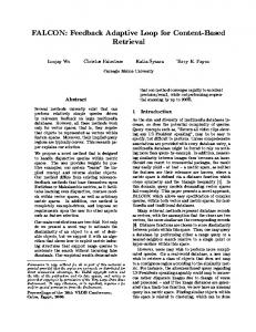
The step marked ⋆ is valid because ✓[−] is itself an evaluation context, being syntactic sugar for let x = [−] in x. Thus we have derived a definition of G, from which we create the following factorised program: reverse = let {rec = G[rec]} in Abs[rec] G[rec] = λxs → λys → case xs of [ ] → ys (z : zs) → let ws = (z : ys) in rec zs ws Expanding this out, we obtain: reverse = let {rec = λxs → λys → case xs of [ ] → ys (z : zs) → let ws = (z : ys) in rec zs ws} in λxs → rec xs [ ] The result is an implementation of fast reverse as a recursive let. The calculations here have essentially the same structure as the correctness proofs, with the addition of some administrative steps to do with the manipulation of ticks. To illustrate the performance gain, we have graphed the performance of the original reverse function against the optimised version in Figure 2. We used the Criterion benchmarking library [18] with a range of list lengths to compare the performance of the two functions The resulting graph shows a clear improvement from quadratic time to linear. We chose to use relatively small list lengths for our graphs, but the trend continues for larger values. 6.2

Tabulating a Function

Our second example is that of tabulating a function by producing a stream (infinite list) of results. Given a function f that takes a natural number as its argument, the tabulate function should produce the following result: [f 0, f 1, f 2, f 3, . . . This function can be implemented in Haskell as follows: tabulate f = f 0 : tabulate (f ◦ (+1)) This definition is inefficient, as it requires that the argument to f be recalculated for each element of the result stream. Essentially, this definition corresponds to the following calculation, involving a significant amount of repeated work: [f 0, f (0 + 1), f ((0 + 1) + 1), f (((0 + 1) + 1) + 1), . . . We wish to apply the worker/wrapper technique to improve the time performance of this program. The first step is to write it as a recursive let in our language:

Figure 2. Performance comparisons of reverse and tabulate tabulate = let {h = F[h]} in h F[M ]

= λf → let {f′ = λx → let {x′ = x + 1} in f x′ } in f 0 : M f′

Next, we must devise Abs and Rep contexts. In order to avoid the repeated work, we hope to derive a version of the tabulate function that takes an additional number argument telling it where to “start” from. The following Abs and Rep contexts convert between these two versions: Abs[M ] = λf → M 0 f Rep[M ] = λn → λf → let {f′ = λx → let {x′ = x + n} in f x′ } ′ in M f Once again, we must introduce some new rules before we can derive the factorised program. Firstly, we require the following two variable substitution rules from [15]: let {x = y} in C [x] ∼ ▷ let {x = y} in C [y] let {x = y} in C [y] ◁▷ let {x = y} in C [x] ≈

Next, we must use some properties of addition. Firstly, we have the following identity properties: x + 0 ◁▷ x ∼ 0 + x ◁▷ x ∼ We also use the following property, combining associativity and commutativity. We shall refer to this as associativity of +. Where t is not free in C, we have: let {t = x + y} in let {r = t + z} in C [r] ◁▷ ∼ let {t = z + y} in let {r = x + t} in C [r] Finally, we use the fact that sums may be floated out of arbitrary contexts. Where z does not occur in C, we have: C [let {z = y + x} in M ] ◁▷ let {z = y + x} in C [M ] ∼

Now we can begin to apply worker/wrapper. Firstly, we verify that Abs and Rep satisfy assumption (B). Again, this is relatively straightforward: Abs[Rep[F[h]]] ≡ { definitions } λf → (λn → λf → let {f′ = λx → let {x′ = x + n} in f x′ } in F[h] f) 0 f′ ◁▷ { β-reduction } ∼ λf → let {f′ = λx → let {x′ = x + 0} in f x′ } ′ in F[h] f ◁▷ { x + 0 ◁▷ x } ≈ ≈ λf → let {f′ = λx → let {x′ = x} in f x′ } ′ in F[h] f ◁▷ { variable substitution, garbage collection } ≈ λf → let {f′ = λx → f x} in F[h] f′ ≡ { defintion of F } λf → let {f′ = λx → f x} in (λf → let {f′′ = λx → let {x′ = x + 1} in f x} ′′ in f 0 : h f ) f′ ◁▷ { β-reduction } ∼ λf → let {f′ = λx → f x} in let {f′′ = λx → let {x′ = x + 1} in f′ x′ } in f′ 0 : h f′′ ◁▷ { value-β on f′ } ≈ λf → let {f′′ = λx → let {x′ = x + 1} in (λx → f x) x′ } in (λx → f x) 0 : h f′′ ◁▷ { β-reduction } ∼ λf → let {f′′ = λx → let {x′ = x + 1} in f x′ } in f 0 : h f′′

in h f′′ ◁▷ { sums float } ∼ λn → λf → f n : let {n′ = n + 1} in ✓let {f′′ = λx → let {x′′ = x + n′ } in f x′′ } in h f′′ ◁▷ { β-expansion, tick floating } ∼ λn → λf → f n : let {n′ = n + 1} in (✓λn → λf → let {f′′ = λx → let {x′ = x + n} in f x′ } in h f′′ ) n′ f ≡ { definition of Rep } λn → λf → f n : let {n′ = n + 1} in (✓Rep[h]) n′ f ≡ { taking this as our definition of G } G[✓Rep[h]]

≡ { definition of F } F[h] Now we use condition (2) to derive the new definition of tabulate. This requires the use of a number of the properties that we presented earlier: Rep[✓F[h]] ≡ { definitions } λn → λf → let {f′ = λx → let {x′ = x + n} in f x′ } ′′ in (^\f → let {f = λx → let {x′′ = x + 1} in f x′′ } in f 0 : h f′′ ) f′ ◁▷ { tick floating [−] f′ } ∼ λn → λf → let {f′ = λx → let {x′ = x + n} in f x′ } ′′ in✓(λf → let {f = λx → let {x′′ = x + 1} in f x′′ } ′′ ′ in f 0 : h f ) f ◁▷ { β-reduction } ∼ λn → λf → let {f′ = λx → let {x′ = x + n} in f x′ } ′′ in✓let {f = λx → let {x′′ = x + 1} in f′ x′′ } in f′ 0 : h f′′ ◁▷ { value-β on f′ , garbage collection } ∼ λn → λf → ✓let {f′′ = λx → let {x′ = x + 1} in (✓λx → let {x′′ = x + n} in f x′′ ) x′ } in (✓λx → let {x′′ = x + n} in f x′′ ) 0 : h f′′ ▷ { removing ticks, β-reduction } ∼ λn → λf → ✓let {f′′ = λx → let {x′ = x + 1} in let {x′′ = x′ + n} in f x′′ } in (let {x′′ = 0 + n} in f x′′ ) : h f′′ ◁▷ { associativity and identity of + } ∼ λn → λf → ✓let {f′′ = λx → let {n′ = n + 1} in let {x′′ = x + n′ } in f x′′ } in (let {x′′ = n} in f x′′ ) : h f′′ ▷ { variable substitution, garbage collection } ∼ λn → λf → ✓let {f′′ = λx → let {n′ = n + 1} in let {x′′ = x + n′ } in f x′′ } in f n : h f′′ ◁▷ { value let-floating } ∼ λn → λf → f n : ✓let {f′′ = λx → let {n′ = n + 1} in let {x′′ = x + n′ } in f x′′ }

Thus we have derived a definition of G, from which we create the following factorised program: tabulate = let {h = G[h]} in Abs[h] G[M ]

= λn → λf → f n : let {n′ = n + 1} in M n′ f

This is the same optimised tabulate function that was proved correct in [10], and the proofs here have a similar structure to the correctness proofs from that paper, except that we have now formalised that the new version of the tabulate function is indeed a time improvement of the original version. We note that the proof of (B) is complicated by the fact that η-reduction is not valid in this setting. In fact, if we assumed η-reduction then our proof of (B) here could be adapted into a proof of (A). We demonstrate the performance gain in Figure 2, again based on Criterion benchmarks. This time, we keep the same input (in this case the function λn → n ∗ n), but vary how many elements of the result stream we evaluate. Once again, we have an improvement from quadratic to linear performance, and the trend continues for larger values.

7.

Related Work

We divide the related work into three sections. Firstly, we discuss various approaches to the operational semantics of lazy languages. Secondly, we discuss the history of improvement theory. Finally, we discuss other approaches that have been used to formally reason about efficiency. 7.1

Lazy Operational Semantics

The notion of call-by-need evaluation was first introduced in 1971 by Wadsworth [30]. However, the semantics most widely regarded as the definition of call-by-need is the natural semantics due to Launchbury [14], which was later used by Sestoft to derive the virtual machine semantics we use in this paper [27]. Ariola, Felleisen, Maraist, Odersky and Wadler presented a call-by-need lambda calculus [1], with operational semantics based on reductions between terms in the source language. This calculus supports an equational theory. However, Moran and Sands showed that this equational theory is subsumed by weak cost-equivalence [15].

7.2

Improvement Theory

Improvement theory was originally developed in 1991 by Sands [21], and applied in a call-by-name setting. In 1997 this was generalised to a wide class of call-by-name and callby-value languages, also by Sands [22]. This theory was also applicable to a general class of resources, rather than just space and time. The theory for lazy languages was developed by Moran and Sands for time efficiency [15] and Gustavsson and Sands for space efficiency [8, 9]. Since the last of these papers was published in 2001, there does not seem to have been much work on improvement theory. We hope that this paper can help to regenerate interest in this topic. 7.3

Formal Reasoning About Efficiency

Okasaki [17] uses techniques of amortised cost analysis to reason about the asymptotic time complexity of lazy functional data structures. This is achieved by modifying analysis techniques such as the Banker’s Method, where the notion of credit is used to spread out the notional cost of an expensive but infrequent operations over more frequent and cheaper operations. The key idea in Okasaki’s work is to invert such techniques to use the notion of debt. This allows the analyses to deal with the persistence of data structures, where the same structure may exist in multiple versions at once. While credit may only be spent once, a single debt may be paid off multiple times (in different versions of the same structure) without risking bankruptcy. These techniques have been used to analyse the asymptotic performance of a number of functional data structures. Sansom and Peyton Jones [24] give a presentation of the GHC profiler, which can be used to measure time as well as space usage of Haskell programs. In doing so, they give a formal cost semantics for GHC Core programs based around the notion of cost centres. Cost centres are a way of annotating expressions, so that the profiler can indicate which parts of the source program cost the most to execute. The cost semantics is used as a specification to develop a precise profiling framework, as well as to prove various properties about cost attribution and verify that certain program transformations do not affect the attribution of costs, though they may of course reduce cost overall. Cost centres are now widely-used in profiling Haskell programs. Hope [11] applies a technique based on instrumenting an abstract machine with cost information to derive a cost semantics for call-by-value functional programs. More specifically, starting from a denotational semantics for the source language, one derives an abstract machine for this language using standard program transformation techniques, instruments this machine with cost information, and then reverses the derivation to arrive at an instrumented denotational semantics. This semantics can then be used to reason about the cost of programs in the high-level source language without reference to the details of the abstract machine. This approach was used to calculate the space and time cost of a range of programming examples, as well as to derive a new deforestation theorem for hylomorphisms.

8.

Conclusion

In this paper, we have shown how improvement theory can be used to justify the worker/wrapper transformation as a program optimisation, by formally proving that, under certain natural conditions, the transformation is guaranteed to preserve or improve time performance. This guarantee is with respect to an established operational semantics for

call-by-need evaluation. We then verified that two examples from previous worker/wrapper papers met the preconditions for this performance guarantee, demonstrating the use of our theory while also verifying the validity of the examples. This work appears to be the first time that rigorous performance guarantees have been given for a general purpose optimisation technique in a call-by-need setting. 8.1

Further Work

As well as for fixed points, worker/wrapper theories also exist for more structured recursion operators such as folds [13] and unfolds [10]. Though the theory we present here can be specialised to such operators, it may be beneficial to investigate this more closely, as doing so may reveal more interesting and subtle details yet to be uncovered. As we mentioned earlier in this paper, a typed theory would be more useful, allowing more power when reasoning about programs. This would also match more closely with the original worker/wrapper theories, which were typed. The key barrier to this is that there is currently no typed improvement theory, so such a theory would have to be developed before the theory here could be made typed. The theory we present here only applies to time efficiency. Gustavsson and Sands have developed an improvement theory for space [8, 9], so this would be an obvious next step for developing our theory. More generally, we could apply a technique such as that used by Sands [22] to develop a theory that applies to a large class of resources, and examine which assumptions must be made about the resources we consider for our theory to apply. Assumptions (A), (B) and (C) are written as weak costequivalences, which limits the scope of our theory to cases where Abs and Rep are fairly simple. We would like to also be able to cover cases where the Abs and Rep contexts correspond to expensive operations, but the extra cost is made up for by the overall efficiency gain of the transformation. To cover such cases, we would require a richer version of improvement theory that is able to quantify how much better one program is than another. As our examples show, the calculations required to derive an improved program can often be quite involved. The HERMIT system, devised by a team at the University of Kansas [6, 26], facilitates program transformations by providing an interactive interface for program transformation that verifies correctness. If improvement theory could be integrated into such a system, it would be significantly easier to apply our worker/wrapper improvement theory. Finally, we are working on a general worker/wrapper theory that will apply to any operator with the property of dinaturality [5]. It is also interesting to consider whether such a general categorical approach can be applied to an operational theory. If this is the case, dinaturality may also provide the necessary machinery to unify the denotational (correctness) and operational (efficiency) theories, which as we have already observed in this paper are very similar in terms of their formulations and proofs. Voigtländer and Johann used parametricity to justify program transformations from a perspective of observational approximation [29]. It may be productive to investigate whether their techniques can be applied to a notion of improvement.

Acknowledgments The authors would like to thank the reviewers as well as Neil Sculthorpe, for their helpful comments on this paper.

References [1] Z. M. Ariola, M. Felleisen, J. Maraist, M. Odersky, and P. Wadler. The Call-by-Need Lambda Calculus. In POPL ’95, pages 233–246. ACM, 1995. [2] R. M. Burstall and J. Darlington. A Transformation System for Developing Recursive Programs. Journal of the ACM, 24 (1):44–67, 1977. [3] K. Claessen and J. Hughes. QuickCheck: A Lightweight Tool for Random Testing of Haskell Programs. In ICFP. ACM, 2000. [4] T. Coquand. Infinite Objects in Type Theory. In TYPES ’93, volume 806 of Lecture Notes in Computer Science. Springer, 1993. [5] E. Dubuc and R. Street. Dinatural Transformations. In Lecture Notes in Mathematics, volume 137 of Lecture Notes in Mathematics, pages 126–137. Springer Berlin Heidelberg, 1970. [6] A. Farmer, A. Gill, E. Komp, and N. Sculthorpe. The HERMIT in the Machine: A Plugin for the Interactive Transformation of GHC Core Language Programs. In Haskell Symposium (Haskell ’12), pages 1–12. ACM, 2012. [7] A. Gill and G. Hutton. The Worker/Wrapper Transformation. Journal of Functional Programming, 19(2), 2009. [8] J. Gustavsson and D. Sands. A Foundation for Space-Safe Transformations of Call-by-Need Programs. Electronic Notes on Theoretical Computer Science, 26:69–86, 1999. [9] J. Gustavsson and D. Sands. Possibilities and Limitations of Call-by-Need Space Improvement. In ICFP, pages 265–276. ACM, 2001. [10] J. Hackett, G. Hutton, and M. Jaskelioff. The Under Performing Unfold: A New Approach to Optimising Corecursive Programs. 2013. To appear in the volume of selected papers from the 25th International Symposium on Implementation and Application of Functional Languages, Nijmegen, The Netherlands, August 2013. [11] C. Hope. A Functional Semantics for Space and Time. PhD thesis, School of Computer Science, University of Nottingham, 2008. [12] J. Hughes. A Novel Representation of Lists and its Application to the Function “reverse”. Information Processing Letters, 22(3):141–144, 1986. [13] G. Hutton, M. Jaskelioff, and A. Gill. Factorising Folds for Faster Functions. Journal of Functional Programming Special Issue on Generic Programming, 20(3&4), June 2010. [14] J. Launchbury. A Natural Semantics for Lazy Evaluation. In POPL ’93, pages 144–154. ACM, 1993. [15] A. Moran and D. Sands. Improvement in a Lazy Context: An Operational Theory for Call-by-Need. Extended version of [16], available at http://citeseerx.ist.psu.edu/viewdoc/ download?doi=10.1.1.37.144&rep=rep1&type=pdf.

[16] A. Moran and D. Sands. Improvement in a Lazy Context: An Operational Theory for Call-by-Need. In POPL ’99, pages 43–56. ACM, 1999. [17] C. Okasaki. Purely Functional Data Structures. Cambridge University Press, 1999. [18] B. O’Sullivan. Criterion, A New Benchmarking Library for Haskell, 2009. URL http://www.serpentine.com/blog/ 2009/09/29/criterion-a-new-benchmarking-libraryfor-haskell/. [19] W. Partain. The nofib Benchmark Suite of Haskell Programs. In Glasgow Workshop on Functional Programming, pages 195–202. Springer, 1992. [20] S. L. Peyton Jones. Compiling Haskell by Program Transformation: A Report from the Trenches. In ESOP, pages 18–44. Springer, 1996. [21] D. Sands. Operational Theories of Improvement in Functional Languages (Extended Abstract). In Glasgow Workshop on Functional Programming, 1991. [22] D. Sands. From SOS Rules to Proof Principles: An Operational Metatheory for Functional Languages. In POPL ’97, pages 428–441. ACM Press, 1997. [23] D. Sands. Improvement Theory and its Applications. In Higher Order Operational Techniques in Semantics, Publications of the Newton Institute. Cambridge University Press, 1997. [24] P. M. Sansom and S. L. Peyton Jones. Formally Based Profiling for Higher-Order Functional Languages. ACM Transactions on Programming Languages and Systems, 19(2), 1997. [25] N. Sculthorpe and G. Hutton. Work It, Wrap It, Fix It, Fold It. Journal of Functional Programming, 2014. [26] N. Sculthorpe, A. Farmer, and A. Gill. The HERMIT in the Tree: Mechanizing Program Transformations in the GHC Core Language. In Proceedings of Implementation and Application of Functional Languages (IFL ’12), volume 8241 of Lecture Notes in Computer Science, pages 86–103, 2013. [27] P. Sestoft. Deriving a Lazy Abstract Machine. Journal of Functional Programming, 7(3):231–264, 1997. [28] D. A. Turner. Elementary Strong Functional Programming. In FPLE ’95, volume 1022 of Lecture Notes in Computer Science. Springer, 1995. [29] J. Voigtländer and P. Johann. Selective Strictness and Parametricity in Structural Operational Semantics, Inequationally. Theor. Comput. Sci., 388(1-3):290–318, 2007. [30] C. P. Wadsworth. Semantics and Pragmatics of the Lambda Calculus. PhD thesis, Computing Laboratory, University of Oxford, 1971. [31] O. Wilde. Lady Windermere’s Fan, A Play About a Good Woman. First performed in 1892.