Working with Time Series Data

Chapter 2

Working with Time Series Data

Chapter Table of Contents TIME SERIES AND SAS DATA SETS . . . . . . . . . . . . . . . . . . . . . 41 Introduction . . . . . . . . . . . . . . . . . . . . . . . . . . . . . . . . . . . 41 Reading a Simple Time Series . . . . . . . . . . . . . . . . . . . . . . . . . 42 DATING OBSERVATIONS . . . . . . . . . . . . . SAS Date, Datetime, and Time Values . . . . . . . Reading Date and Datetime Values with Informats . Formatting Date and Datetime Values . . . . . . . The Variables DATE and DATETIME . . . . . . . Sorting by Time . . . . . . . . . . . . . . . . . . .

. . . . . .

. . . . . .

. . . . . .

. . . . . .

. . . . . .

. . . . . .

. . . . . .

. . . . . .

. . . . . .

43 44 45 46 47 48

SUBSETTING DATA AND SELECTING OBSERVATIONS Subsetting SAS Data Sets . . . . . . . . . . . . . . . . . . . . Using the WHERE Statement with SAS Procedures . . . . . . Using SAS Data Set Options . . . . . . . . . . . . . . . . . .

. . . .

. . . .

. . . .

. . . .

. . . .

. . . .

. . . .

. . . .

48 49 50 50

STORING TIME SERIES IN A SAS DATA SET Standard Form of a Time Series Data Set . . . . Several Series with Different Ranges . . . . . . . Missing Values and Omitted Observations . . . . Cross-sectional Dimensions and BY Groups . . . Interleaved Time Series . . . . . . . . . . . . . . Output Data Sets of SAS/ETS Procedures . . . .

. . . . . . .

. . . . . . .

. . . . . . .

. . . . . . .

. . . . . . .

. . . . . . .

. . . . . . .

. . . . . . .

51 52 53 53 54 56 58

TIME SERIES PERIODICITY AND TIME INTERVALS . . . . . . . . . . Specifying Time Intervals . . . . . . . . . . . . . . . . . . . . . . . . . . . . Using Time Intervals with SAS/ETS Procedures . . . . . . . . . . . . . . . . Time Intervals, the Time Series Forecasting System and the Time Series Viewer

60 61 61 62

PLOTTING TIME SERIES . . Using the Time Series Viewer Using PROC GPLOT . . . . . Using PROC PLOT . . . . . . Using PROC TIMEPLOT . . .

63 63 63 69 76

. . . . .

. . . . .

. . . . .

. . . . .

. . . . .

. . . . .

. . . . .

. . . . .

. . . . .

. . . . .

. . . . . . .

. . . . .

. . . . . .

. . . . . . .

. . . . .

. . . . . .

. . . . . . .

. . . . .

. . . . . .

. . . . . . .

. . . . .

. . . . . .

. . . . . . .

. . . . .

. . . . . .

. . . . . . .

. . . . .

. . . . . . .

. . . . .

. . . . .

. . . . .

. . . . .

. . . . .

. . . . .

. . . . .

. . . . .

. . . . .

CALENDAR AND TIME FUNCTIONS . . . . . . . . . . . . . . . . . . . . 77 Computing Dates from Calendar Variables . . . . . . . . . . . . . . . . . . . 77 39

Part 1. General Information Computing Calendar Variables from Dates . . . . . . Converting between Date, Datetime, and Time Values Computing Datetime Values . . . . . . . . . . . . . Computing Calendar and Time Variables . . . . . . .

. . . .

. . . .

. . . .

. . . .

. . . .

. . . .

. . . .

. . . .

. . . .

. . . .

. . . .

. . . .

78 79 79 79

INTERVAL FUNCTIONS INTNX AND INTCK . . . . Incrementing Dates by Intervals . . . . . . . . . . . . . Alignment of SAS Dates . . . . . . . . . . . . . . . . . Computing the Width of a Time Interval . . . . . . . . . Computing the Ceiling of an Interval . . . . . . . . . . . Counting Time Intervals . . . . . . . . . . . . . . . . . Checking Data Periodicity . . . . . . . . . . . . . . . . Filling in Omitted Observations in a Time Series Data Set Using Interval Functions for Calendar Calculations . . .

. . . . . . . . .

. . . . . . . . .

. . . . . . . . .

. . . . . . . . .

. . . . . . . . .

. . . . . . . . .

. . . . . . . . .

. . . . . . . . .

. . . . . . . . .

. . . . . . . . .

. . . . . . . . .

80 81 83 84 85 85 86 86 87

LAGS, LEADS, DIFFERENCES, AND SUMMATIONS The LAG and DIF Functions . . . . . . . . . . . . . . . Multiperiod Lags and Higher-Order Differencing . . . . Percent Change Calculations . . . . . . . . . . . . . . . Leading Series . . . . . . . . . . . . . . . . . . . . . . Summing Series . . . . . . . . . . . . . . . . . . . . . .

. . . . . .

. . . . . .

. . . . . .

. . . . . .

. . . . . .

. . . . . .

. . . . . .

. . . . . .

. . . . . .

. . . . . .

. . . . . .

88 88 92 92 94 95

TRANSFORMING TIME SERIES . . . . . . . . . Log Transformation . . . . . . . . . . . . . . . . . Other Transformations . . . . . . . . . . . . . . . The EXPAND Procedure and Data Transformations

. . . .

. . . .

. . . .

. . . .

. . . .

. . . .

. . . .

. . . .

. . . .

. . . .

. . . .

97 98 99 100

. . . .

. . . .

. . . .

. . . .

MANIPULATING TIME SERIES DATA SETS . . . . . . . . . . . . . . . . 100 Splitting and Merging Data Sets . . . . . . . . . . . . . . . . . . . . . . . . 100 Transposing Data Sets . . . . . . . . . . . . . . . . . . . . . . . . . . . . . 101 TIME SERIES INTERPOLATION . . . . . . . . . . . . . Interpolating Missing Values . . . . . . . . . . . . . . . . Interpolating to a Higher or Lower Frequency . . . . . . . Interpolating between Stocks and Flows, Levels and Rates

. . . .

. . . .

. . . .

. . . .

. . . .

. . . .

. . . .

. . . .

. . . .

. . . .

105 105 106 106

READING TIME SERIES DATA . . . . . . . . . . . . . . . . . . . . . . . . 107 Reading a Simple List of Values . . . . . . . . . . . . . . . . . . . . . . . . 107 Reading Fully Described Time Series in Transposed Form . . . . . . . . . . 107

SAS OnlineDoc: Version 8

40

Chapter 2

Working with Time Series Data This chapter discusses working with time series data in the SAS System. The following topics are included: dating time series and working with SAS date and datetime values subsetting data and selecting observations storing time series data in SAS data sets specifying time series periodicity and time intervals plotting time series using calendar and time interval functions computing lags and other functions across time transforming time series transposing time series data sets interpolating time series reading time series data recorded in different ways

In general, this chapter focuses on using features of the SAS programming language and not on features of SAS/ETS software. However, since SAS/ETS procedures are used to analyze time series, understanding how to use the SAS programming language to work with time series data is important for the effective use of SAS/ETS software. You do not need to read this chapter to use SAS/ETS procedures. If you are already familiar with SAS programming you may want to skip this chapter, or you may refer to sections of this chapter for help on specific time series data processing questions.

Time Series and SAS Data Sets Introduction To analyze data with the SAS System, data values must be stored in a SAS data set. A SAS data set is a matrix or table of data values organized into variables and observations. The variables in a SAS data set label the columns of the data matrix and the observations in a SAS data set are the rows of the data matrix. You can also think of a SAS data set as a kind of file, with the observations representing records in the file and the variables representing fields in the records. (Refer to SAS Language: Reference, Version 6 for more information about SAS data sets.) 41

Part 1. General Information Usually, each observation represents the measurement of one or more variables for the individual subject or item observed. Often, the values of some of the variables in the data set are used to identify the individual subjects or items that the observations measure. These identifying variables are referred to as ID variables. For many kinds of statistical analysis, only relationships among the variables are of interest, and the identity of the observations does not matter. ID variables may not be relevant in such a case. However, for time series data the identity and order of the observations are crucial. A time series is a set of observations made at a succession of equally spaced points in time. For example, if the data are monthly sales of a company’s product, the variable measured is sales of the product and the thing observed is the operation of the company during each month. These observations can be identified by year and month. If the data are quarterly gross national product, the variable measured is final goods production and the thing observed is the economy during each quarter. These observations can be identified by year and quarter. For time series data, the observations are identified and related to each other by their position in time. Since the SAS system does not assume any particular structure to the observations in a SAS data set, there are some special considerations needed when storing time series in a SAS data set. The main considerations are how to associate dates with the observations and how to structure the data set so that SAS/ETS procedures and other SAS procedures will recognize the observations of the data set as constituting time series. These issues are discussed in following sections.

Reading a Simple Time Series Time series data can be recorded in many different ways. The section "Reading Time Series Data" later in this chapter discusses some of the possibilities. The example below shows a simple case. The following SAS statements read monthly values of the U.S. Consumer Price Index for June 1990 through July 1991. The data set USCPI is shown in Figure 2.1. data uscpi; input year month cpi; datalines; 1990 6 129.9 1990 7 130.4 1990 8 131.6 1990 9 132.7 1990 10 133.5 1990 11 133.8 1990 12 133.8 1991 1 134.6 1991 2 134.8 1991 3 135.0


42

Chapter 2. Dating Observations 1991 1991 1991 1991 ;

4 5 6 7

135.2 135.6 136.0 136.2

proc print data=uscpi; run;

Figure 2.1.

Obs

year

1 2 3 4 5 6 7 8 9 10 11 12 13 14

1990 1990 1990 1990 1990 1990 1990 1991 1991 1991 1991 1991 1991 1991

month 6 7 8 9 10 11 12 1 2 3 4 5 6 7

cpi 129.9 130.4 131.6 132.7 133.5 133.8 133.8 134.6 134.8 135.0 135.2 135.6 136.0 136.2

Time Series Data

When a time series is stored in the manner shown by this example, the terms series and variable can be used interchangeably. There is one observation per row, and one series/variable per column.

Dating Observations The SAS System supports special date, datetime, and time values, which make it easy to represent dates, perform calendar calculations, and identify the time period of observations in a data set. The preceding example used the ID variables YEAR and MONTH to identify the time periods of the observations. For a quarterly data set, you might use YEAR and QTR as ID variables. A daily data set might have the ID variables YEAR, MONTH, and DAY. Clearly, it would be more convenient to have a single ID variable that could be used to identify the time period of observations, regardless of their frequency. The following section, "SAS Date, Datetime, and Time Values," discusses how the SAS System represents dates and times internally and how to specify date, datetime, and time values in a SAS program. The section "Reading Date and Datetime Values with Informats" discusses how to control the display of date and datetime values in SAS output and how to read in date and time values from data records. Later sections discuss other issues concerning date and datetime values, specifying time intervals, data periodicity, and calendar calculations.

43


Part 1. General Information SAS date and datetime values and the other features discussed in the following sections are also described in SAS Language: Reference. Reference documentation on these features is also provided in Chapter 3, “Date Intervals, Formats, and Functions,”.

SAS Date, Datetime, and Time Values Year 2000 Compliance SAS software correctly represents dates from 1582 AD to the year 20,000 AD. If dates in an external data source are represented with four-digit-year values SAS can read, write and compute these dates. If the dates in an external data source are twodigit years, SAS software provides informats, functions, and formats to read, manipulate, and output dates that are Year 2000 compliant. The YEARCUTOFF= system option can also be used to interpret dates with two-digit years by specifying the first year of a 100-year span that will be used in informats and functions. The default value for the YEARCUTOFF= option is 1920. SAS Date Values The SAS System represents dates as the number of days since a reference date. The reference date, or date zero, used for SAS date values is 1 January 1960. Thus, for example, 3 February 1960 is represented by the SAS System as 33. The SAS date for 17 October 1991 is 11612. Dates represented in this way are called SAS date values. Any numeric variable in a SAS data set whose values represent dates in this way is called a SAS date variable. Representing dates as the number of days from a reference date makes it easy for the computer to store them and perform calendar calculations, but these numbers are not meaningful to users. However, you never have to use SAS date values directly, since SAS automatically converts between this internal representation and ordinary ways of expressing dates, provided that you indicate the format with which you want the date values to be displayed. (Formatting of date values is explained in a following section.)

SAS Date Constants SAS date values are written in a SAS program by placing the dates in single quotes followed by a D. The date is represented by the day of the month, the three letter abbreviation of the month name, and the year. For example, SAS reads the value ’17OCT1991’D the same as 11612, the SAS date value for 17 October 1991. Thus, the following SAS statements print DATE=11612. data _null_; date = ’17oct1991’d; put date=; run;

The year value can be given with two or four digits, so ’17OCT91’D is the same as ’17OCT1991’D. (The century assumed for a two-digit year value can be controlled with the YEARCUTOFF= option in the OPTIONS statement. Refer to the SAS Language: Reference for information on YEARCUTOFF=.) SAS OnlineDoc: Version 8

44

Chapter 2. Dating Observations SAS Datetime Values and Datetime Constants To represent both the time of day and the date, the SAS System uses datetime values. SAS datetime values represent the date and time as the number of seconds the time is from a reference time. The reference time, or time zero, used for SAS datetime values is midnight, 1 January 1960. Thus, for example, the SAS datetime value for 17 October 1991 at 2:45 in the afternoon is 1003329900. To specify datetime constants in a SAS program, write the date and time in single quotes followed by DT. To write the date and time in a SAS datetime constant, write the date part using the same syntax as for date constants, and follow the date part with the hours, the minutes, and the seconds, separating the parts with colons. The seconds are optional. For example, in a SAS program you would write 17 October 1991 at 2:45 in the afternoon as ’17OCT91:14:45’DT. SAS reads this as 1003329900. Table 2.1 shows some other examples of datetime constants. Table 2.1.

Examples of Datetime Constants

Datetime Constant ’17OCT1991:14:45:32’DT ’17OCT1991:12:5’DT ’17OCT1991:2:0’DT ’17OCT1991:0:0’DT

Time 32 seconds past 2:45 p.m., 17 October 1991 12:05 p.m., 17 October 1991 2 AM, 17 October 1991 midnight, 17 October 1991

SAS Time Values The SAS System also supports time values. SAS time values are just like datetime values, except that the date part is not given. To write a time value in a SAS program, write the time the same as for a datetime constant but use T instead of DT. For example, 2:45:32 p.m. is written ’14:45:32’T. Time values are represented by a number of seconds since midnight, so SAS reads ’14:45:32’T as 53132. SAS time values are not very useful for identifying time series, since usually both the date and the time of day are needed. Time values are not discussed further in this book.

Reading Date and Datetime Values with Informats The SAS System provides a selection of informats for reading SAS date and datetime values from date and time values recorded in ordinary notations. A SAS informat is an instruction that converts the values from a character string representation into the internal numerical value of a SAS variable. Date informats convert dates from ordinary notations used to enter them to SAS date values; datetime informats convert date and time from ordinary notation to SAS datetime values. For example, the following SAS statements read monthly values of the U.S. Consumer Price Index. Since the data are monthly, you could identify the date with the variables YEAR and MONTH, as in the previous example. Instead, in this example the time periods are coded as a three-letter month abbreviation followed by the year. The informat MONYY. is used to read month-year dates coded this way and to express them as SAS date values for the first day of the month, as follows.

45


Part 1. General Information data uscpi; input date: monyy7. cpi; datalines; jun1990 129.9 jul1990 130.4 aug1990 131.6 sep1990 132.7 oct1990 133.5 nov1990 133.8 dec1990 133.8 jan1991 134.6 feb1991 134.8 mar1991 135.0 apr1991 135.2 may1991 135.6 jun1991 136.0 jul1991 136.2 ;

The SAS System provides informats for most common notations for dates and times. See Chapter 3 for more information on the date and datetime informats available.

Formatting Date and Datetime Values The SAS System provides formats to convert the internal representation of date and datetime values used by SAS to ordinary notations for dates and times. Several different formats are available for displaying dates and datetime values in most of the commonly used notations. A SAS format is aan instruction that converts the internal numerical value of a SAS variable to a character string that can be printed or displayed. Date formats convert SAS date values to a readable form; datetime formats convert SAS datetime values to a readable form. In the preceding example, the variable DATE was set to the SAS date value for the first day of the month for each observation. If the data set USCPI were printed or otherwise displayed, the values shown for DATE would be the number of days since 1 January 1960. (See the "DATE with no format" column in Figure 2.2.) To display date values appropriately, use the FORMAT statement. The following example processes the data set USCPI to make several copies of the variable DATE and uses a FORMAT statement to give different formats to these copies. The format cases shown are the MONYY7. format (for the DATE variable), the DATE9. format (for the DATE1 variable), and no format (for the DATE0 variable). The PROC PRINT output in Figure 2.2 shows the effect of the different formats on how the date values are printed. data fmttest; set uscpi; date0 = date; date1 = date;


46

Chapter 2. Dating Observations label date date1 date0 format date run;

= "DATE = "DATE = "DATE monyy7.

with MONYY7. format" with DATE9. format" with no format"; date1 date9.;

proc print data=fmttest label; run;

Obs 1 2 3 4 5 6 7 8 9 10

Figure 2.2.

DATE with MONYY. format JUN1990 JUL1990 AUG1990 SEP1990 OCT1990 NOV1990 DEC1990 JAN1991 FEB1991 MAR1991

cpi

DATE with no format

DATE with DATE. format

129.9 130.4 131.6 132.7 133.5 133.8 133.8 134.6 134.8 135.0

11109 11139 11170 11201 11231 11262 11292 11323 11354 11382

01JUN1990 01JUL1990 01AUG1990 01SEP1990 01OCT1990 01NOV1990 01DEC1990 01JAN1991 01FEB1991 01MAR1991

SAS Date Values Printed with Different Formats

The appropriate format to use for SAS date or datetime valued ID variables depends on the sampling frequency or periodicity of the time series. Table 2.2 shows recommended formats for common data sampling frequencies and shows how the date ’17OCT1991’D or the datetime value ’17OCT1991:14:45:32’DT is displayed by these formats. Table 2.2.

Formats for Different Sampling Frequencies

ID values SAS Date

SAS Datetime

Periodicity Annual Quarterly Monthly Weekly Daily Hourly Minutes Seconds

FORMAT YEAR4. YYQC6. MONYY7. WEEKDATX23. DATE9. DATE9. DATETIME10. DATETIME13. DATETIME16.

Example 1991 1991:4 OCT1991 Thursday, 17 Oct 1991 17OCT1991 17OCT1991 17OCT91:14 17OCT91:14:45 17OCT91:14:45:32

See Chapter 3 for more information on the date and datetime formats available.

The Variables DATE and DATETIME SAS/ETS procedures enable you to identify time series observations in many different ways to suit your needs. As discussed in preceding sections, you can use a combination of several ID variables, such as YEAR and MONTH for monthly data. However, using a single SAS date or datetime ID variable is more convenient and enables you to take advantage of some features SAS/ETS procedures provide for pro-

47


Part 1. General Information cessing ID variables. One such feature is automatic extrapolation of the ID variable to identify forecast observations. These features are discussed in following sections. Thus, it is a good practice to include a SAS date or datetime ID variable in all the time series SAS data sets you create. It is also a good practice to always give the date or datetime ID variable a format appropriate for the data periodicity. You can name a SAS date or datetime valued ID variable any name conforming to SAS variable name requirements. However, you may find working with time series data in SAS easier and less confusing if you adopt the practice of always using the same name for the SAS date or datetime ID variable. This book always names the dating ID variable "DATE" if it contains SAS date values or "DATETIME" if it contains SAS datetime values. This makes it easy to recognize the ID variable and also makes it easy to recognize whether this ID variable uses SAS date or datetime values.

Sorting by Time Many SAS/ETS procedures assume the data are in chronological order. If the data are not in time order, you can use the SORT procedure to sort the data set. For example proc sort data=a; by date; run;

There are many ways of coding the time ID variable or variables, and some ways do not sort correctly. If you use SAS date or datetime ID values as suggested in the preceding section, you do not need to be concerned with this issue. But if you encode date values in nonstandard ways, you need to consider whether your ID variables will sort. SAS date and datetime values always sort correctly, as do combinations of numeric variables like YEAR, MONTH, and DAY used together. Julian dates also sort correctly. (Julian dates are numbers of the form yyddd, where yy is the year and ddd is the day of the year. For example 17 October 1991 has the Julian date value 91290.) Calendar dates such as numeric values coded as mmddyy or ddmmyy do not sort correctly. Character variables containing display values of dates, such as dates in the notation produced by SAS date formats, generally do not sort correctly.

Subsetting Data and Selecting Observations It is often necessary to subset data for analysis. You may need to subset data to restrict the time range. For example, you want to perform a time series analysis using only recent data and ignoring observations from the distant past. select cross sections of the data. (See the section "Cross-sectional Dimensions and BY Groups" later in this chapter.) For example, you have a data set with SAS OnlineDoc: Version 8

48

Chapter 2. Subsetting Data and Selecting Observations observations over time for each of several states, and you want to analyze the data for a single state. select particular kinds of time series from an interleaved form data set. (See the section "Interleaved Time Series and the – TYPE– Variable" later in this chapter.) For example, you have an output data set produced by the FORECAST procedure that contains both forecast and confidence limits observations, and you want to extract only the forecast observations. exclude particular observations. For example, you have an outlier in your time series, and you want to exclude this observation from the analysis.

You can subset data either by using the DATA step to create a subset data set or by using a WHERE statement with the SAS procedure that analyzes the data. A typical WHERE statement used in a procedure has the form proc arima data=full; where ’31dec1993’d < day < ’26mar1994’d; identify var=close; run;

For complete reference documentation on the WHERE statement refer to SAS Language: Reference.

Subsetting SAS Data Sets To create a subset data set, specify the name of the subset data set on the DATA statement, bring in the full data set with a SET statement, and specify the subsetting criteria with either subsetting IF statements or WHERE statements. For example, suppose you have a data set containing time series observations for each of several states. The following DATA step uses a WHERE statement to exclude observations with dates before 1970 and uses a subsetting IF statement to select observations for the state NC: data subset; set full; where date >= ’1jan1970’d; if state = ’NC’; run;

In this case, it makes no difference logically whether the WHERE statement or the IF statement is used, and you can combine several conditions on one subsetting statement. The following statements produce the same results as the previous example: data subset; set full; if date >= ’1jan1970’d & state = ’NC’; run;

49


Part 1. General Information The WHERE statement acts on the input data sets specified in the SET statement before observations are processed by the DATA step program, whereas the IF statement is executed as part of the DATA step program. If the input data set is indexed, using the WHERE statement can be more efficient than using the IF statement. However, the WHERE statement can only refer to variables in the input data set, not to variables computed by the DATA step program. To subset the variables of a data set, use KEEP or DROP statements or use KEEP= or DROP= data set options. Refer to SAS Language: Reference for information on KEEP and DROP statements and SAS data set options. For example, suppose you want to subset the data set as in the preceding example, but you want to include in the subset data set only the variables DATE, X, and Y. You could use the following statements: data subset; set full; if date >= ’1jan1970’d & state = ’NC’; keep date x y; run;

Using the WHERE Statement with SAS Procedures Use the WHERE statement with SAS procedures to process only a subset of the input data set. For example, suppose you have a data set containing monthly observations for each of several states, and you want to use the AUTOREG procedure to analyze data since 1970 for the state NC. You could use the following: proc autoreg data=full; where date >= ’1jan1970’d & state = ’NC’; ... additional statements ... run;

You can specify any number of conditions on the WHERE statement. For example, suppose that a strike created an outlier in May 1975, and you want to exclude that observation. You could use the following: proc autoreg data=full; where date >= ’1jan1970’d & state = ’NC’ & date ^= ’1may1975’d; ... additional statements ... run;

Using SAS Data Set Options You can use the OBS= and FIRSTOBS= data set options to subset the input data set. (These options cannot be used in conjunction with the WHERE statement.) For example, the following statements print observations 20 through 25 of the data set FULL. SAS OnlineDoc: Version 8

50

Chapter 2. Storing Time Series in a SAS Data Set proc print data=full(firstobs=20 obs=25); run;

You can use KEEP= and DROP= data set options to exclude variables from the input data set. Refer to SAS Language: Reference for information on SAS data set options.

Storing Time Series in a SAS Data Set This section discusses aspects of storing time series in SAS data sets. The topics discussed are the standard form of a time series data set, storing several series with different time ranges in the same data set, omitted observations, cross-sectional dimensions and BY groups, and interleaved time series. Any number of time series can be stored in a SAS data set. Normally, each time series is stored in a separate variable. For example, the following statements augment the USCPI data set read in the previous example with values for the producer price index. data usprice; input date monyy7. cpi ppi; format date monyy7.; label cpi = "Consumer Price Index" ppi = "Producer Price Index"; datalines; jun1990 129.9 114.3 jul1990 130.4 114.5 aug1990 131.6 116.5 sep1990 132.7 118.4 oct1990 133.5 120.8 nov1990 133.8 120.1 dec1990 133.8 118.7 jan1991 134.6 119.0 feb1991 134.8 117.2 mar1991 135.0 116.2 apr1991 135.2 116.0 may1991 135.6 116.5 jun1991 136.0 116.3 jul1991 136.2 116.0 ; proc print data=usprice; run;

51


Part 1. General Information

Figure 2.3.

Obs

date

1 2 3 4 5 6 7 8 9 10 11 12 13 14

JUN1990 JUL1990 AUG1990 SEP1990 OCT1990 NOV1990 DEC1990 JAN1991 FEB1991 MAR1991 APR1991 MAY1991 JUN1991 JUL1991

cpi

ppi

129.9 130.4 131.6 132.7 133.5 133.8 133.8 134.6 134.8 135.0 135.2 135.6 136.0 136.2

114.3 114.5 116.5 118.4 120.8 120.1 118.7 119.0 117.2 116.2 116.0 116.5 116.3 116.0

Time Series Data Set Containing Two Series

Standard Form of a Time Series Data Set The simple way the CPI and PPI time series are stored in the USPRICE data set in the preceding example is termed the standard form of a time series data set. A time series data set in standard form has the following characteristics: The data set contains one variable for each time series. The data set contains exactly one observation for each time period. The data set contains an ID variable or variables that identify the time period of each observation. The data set is sorted by the ID variables associated with date time values, so the observations are in time sequence. The data are equally spaced in time. That is, successive observations are a fixed time interval apart, so the data set can be described by a single sampling interval such as hourly, daily, monthly, quarterly, yearly, and so forth. This means that time series with different sampling frequencies are not mixed in the same SAS data set.

Most SAS/ETS procedures that process time series expect the input data set to contain time series in this standard form, and this is the simplest way to store time series in SAS data sets. There are more complex ways to represent time series in SAS data sets. You can incorporate cross-sectional dimensions with BY groups, so that each BY group is like a standard form time series data set. This method is discussed in the section "Cross-sectional Dimensions and BY Groups." You can interleave time series, with several observations for each time period identified by another ID variable. Interleaved time series data sets are used to store several series in the same SAS variable. Interleaved time series data sets are often used to store series of actual values, predicted values, and residuals, or series of forecast values and confidence limits for the forecasts. This is discussed in the section "Interleaved Time Series and the – TYPE– Variable" later in this chapter. SAS OnlineDoc: Version 8

52

Chapter 2. Storing Time Series in a SAS Data Set

Several Series with Different Ranges Different time series can have values recorded over different time ranges. Since a SAS data set must have the same observations for all variables, when time series with different ranges are stored in the same data set, missing values must be used for the periods in which a series is not available. Suppose that in the previous example you did not record values for CPI before August 1990 and did not record values for PPI after June 1991. The USPRICE data set could be read with the following statements: data usprice; input date monyy7. cpi ppi; format date monyy7.; datalines; jun1990 . 114.3 jul1990 . 114.5 aug1990 131.6 116.5 sep1990 132.7 118.4 oct1990 133.5 120.8 nov1990 133.8 120.1 dec1990 133.8 118.7 jan1991 134.6 119.0 feb1991 134.8 117.2 mar1991 135.0 116.2 apr1991 135.2 116.0 may1991 135.6 116.5 jun1991 136.0 116.3 jul1991 136.2 . ;

The decimal points with no digits in the data records represent missing data and are read by the SAS System as missing value codes. In this example, the time range of the USPRICE data set is June 1990 through July 1991, but the time range of the CPI variable is August 1990 through July 1991, and the time range of the PPI variable is June 1990 through June 1991. SAS/ETS procedures ignore missing values at the beginning or end of a series. That is, the series is considered to begin with the first nonmissing value and end with the last nonmissing value.

Missing Values and Omitted Observations Missing data can also occur within a series. Missing values that appear after the beginning of a time series and before the end of the time series are called embedded missing values. Suppose that in the preceding example you did not record values for CPI for November 1990 and did not record values for PPI for both November 1990 and March 1991. The USPRICE data set could be read with the following statements.

53


Part 1. General Information data usprice; input date monyy. cpi ppi; format date monyy.; datalines; jun1990 . 114.3 jul1990 . 114.5 aug1990 131.6 116.5 sep1990 132.7 118.4 oct1990 133.5 120.8 nov1990 . . dec1990 133.8 118.7 jan1991 134.6 119.0 feb1991 134.8 117.2 mar1991 135.0 . apr1991 135.2 116.0 may1991 135.6 116.5 jun1991 136.0 116.3 jul1991 136.2 . ;

In this example, the series CPI has one embedded missing value, and the series PPI has two embedded missing values. The ranges of the two series are the same as before. Note that the observation for November 1990 has missing values for both CPI and PPI; there is no data for this period. This is an example of a missing observation. You might ask why the data record for this period is included in the example at all, since the data record contains no data. However, if the data record for November 1990 were deleted from the example, this would cause an omitted observation in the USPRICE data set. SAS/ETS procedures expect input data sets to contain observations for a contiguous time sequence. If you omit observations from a time series data set and then try to analyze the data set with SAS/ETS procedures, the omitted observations will cause errors. When all data are missing for a period, a missing observation should be included in the data set to preserve the time sequence of the series.

Cross-sectional Dimensions and BY Groups Often, a collection of time series are related by a cross-sectional dimension. For example, the national average U.S. consumer price index data shown in the previous example can be disaggregated to show price indexes for major cities. In this case there are several related time series: CPI for New York, CPI for Chicago, CPI for Los Angeles, and so forth. When these time series are considered one data set, the city whose price level is measured is a cross-sectional dimension of the data. There are two basic ways to store such related time series in a SAS data set. The first way is to use a standard form time series data set with a different variable for each series.


54

Chapter 2. Storing Time Series in a SAS Data Set For example, the following statements read CPI series for three major U.S. cities: data citycpi; input date monyy7. cpiny cpichi cpila; format date monyy7.; datalines; nov1989 133.200 126.700 130.000 dec1989 133.300 126.500 130.600 jan1990 135.100 128.100 132.100 feb1990 135.300 129.200 133.600 mar1990 136.600 129.500 134.500 apr1990 137.300 130.400 134.200 may1990 137.200 130.400 134.600 jun1990 137.100 131.700 135.000 jul1990 138.400 132.000 135.600 ;

The second way is to store the data in a time series cross-sectional form. In this form, the series for all cross sections are stored in one variable and a cross-section ID variable is used to identify observations for the different series. The observations are sorted by the cross-section ID variable and by time within each cross section. The following statements indicate how to read the CPI series for U.S. cities in time series cross-sectional form: data cpicity; input city $11. date monyy7. cpi; format date monyy7.; datalines; Chicago nov1989 126.700 Chicago dec1989 126.500 Chicago jan1990 128.100 Chicago feb1990 129.200 Chicago mar1990 129.500 Chicago apr1990 130.400 Chicago may1990 130.400 Chicago jun1990 131.700 Chicago jul1990 132.000 Los Angeles nov1989 130.000 Los Angeles dec1989 130.600 Los Angeles jan1990 132.100 ... etc. ... New York may1990 137.200 New York jun1990 137.100 New York jul1990 138.400 ; proc sort data=cpicity; by city date; run;

55


Part 1. General Information When processing a time series cross-section-form data set with most SAS/ETS procedures, use the cross-section ID variable in a BY statement to process the time series separately. The data set must be sorted by the cross-section ID variable and sorted by date within each cross section. The PROC SORT step in the preceding example ensures that the CPICITY data set is correctly sorted. When the cross-section ID variable is used in a BY statement, each BY group in the data set is like a standard form time series data set. Thus, SAS/ETS procedures that expect a standard form time series data set can process time series cross-sectional data sets when a BY statement is used, producing an independent analysis for each cross section. It is also possible to analyze time series cross-sectional data jointly. The TSCSREG procedure expects the input data to be in the time series cross-sectional form described here. See Chapter 20 for more information.

Interleaved Time Series Normally, a time series data set has only one observation for each time period, or one observation for each time period within a cross section for a time series crosssectional form data set. However, it is sometimes useful to store several related time series in the same variable when the different series do not correspond to levels of a cross-sectional dimension of the data. In this case, the different time series can be interleaved. An interleaved time series data set is similar to a time series cross-sectional data set, except that the observations are sorted differently, and the ID variable that distinguishes the different time series does not represent a cross-sectional dimension. Some SAS/ETS procedures produce interleaved output data sets. The interleaved time series form is a convenient way to store procedure output when the results consist of several different kinds of series for each of several input series. (Interleaved time series are also easy to process with plotting procedures. See the section "Plotting Time Series" later in this chapter.) For example, the FORECAST procedure fits a model to each input time series and computes predicted values and residuals from the model. The FORECAST procedure then uses the model to compute forecast values beyond the range of the input data and also to compute upper and lower confidence limits for the forecast values. Thus, the output from PROC FORECAST consists of five related time series for each variable forecast. The five resulting time series for each input series are stored in a single output variable with the same name as the input series being forecast. The observations for the five resulting series are identified by values of the ID variable – TYPE– . These observations are interleaved in the output data set with observations for the same date grouped together. The following statements show the use of PROC FORECAST to forecast the variable CPI in the USCPI data set. Figure 2.4 shows part of the output data set produced by PROC FORECAST and illustrates the interleaved structure of this data set.


56

Chapter 2. Storing Time Series in a SAS Data Set proc forecast data=uscpi interval=month lead=12 out=foreout outfull outresid; var cpi; id date; run; proc print data=foreout; run;

Obs

date

37 38 39 40 41 42 43 44 45 46 47 48

JUN1991 JUN1991 JUN1991 JUL1991 JUL1991 JUL1991 AUG1991 AUG1991 AUG1991 SEP1991 SEP1991 SEP1991

Figure 2.4.

_TYPE_ ACTUAL FORECAST RESIDUAL ACTUAL FORECAST RESIDUAL FORECAST L95 U95 FORECAST L95 U95

_LEAD_ 0 0 0 0 0 0 1 1 1 2 2 2

cpi 136.000 136.146 -0.146 136.200 136.566 -0.366 136.856 135.723 137.990 137.443 136.126 138.761

Partial Listing of Output Data Set Produced by PROC FORECAST

Observations with – TYPE– =ACTUAL contain the values of CPI read from the input data set. Observations with – TYPE– =FORECAST contain one-step-ahead predicted values for observations with dates in the range of the input series, and contain forecast values for observations for dates beyond the range of the input series. Observations with – TYPE– =RESIDUAL contain the difference between the actual and one-stepahead predicted values. Observations with – TYPE– =U95 and – TYPE– =L95 contain the upper and lower bounds of the 95% confidence interval for the forecasts.

Using Interleaved Data Sets as Input to SAS/ETS Procedures Interleaved time series data sets are not directly accepted as input by SAS/ETS procedures. However, it is easy to use a WHERE statement with any procedure to subset the input data and select one of the interleaved time series as the input. For example, to analyze the residual series contained in the PROC FORECAST output data set with another SAS/ETS procedure, include a WHERE – TYPE– =’RESIDUAL’; statement. The following statements perform a spectral analysis of the residuals produced by PROC FORECAST in the preceding example: proc spectra data=foreout out=spectout; var cpi; where _type_=’RESIDUAL’; run;

Combined Cross Sections and Interleaved Time Series Data Sets Interleaved time series output data sets produced from BY-group processing of time series cross-sectional input data sets have a complex structure combining a crosssectional dimension, a time dimension, and the values of the – TYPE– variable. For example, consider the PROC FORECAST output data set produced by the following. 57


Part 1. General Information data cpicity; input city $11. date monyy7. cpi; format date monyy7.; datalines; Chicago nov1989 126.700 Chicago dec1989 126.500 Chicago jan1990 128.100 ... etc. ... New York may1990 137.200 New York jun1990 137.100 New York jul1990 138.400 ; proc sort data=cpicity; by city date; run; proc forecast data=cpicity interval=month lead=2 out=foreout outfull outresid; var cpi; id date; by city; run;

The output data set FOREOUT contains many different time series in the single variable CPI. BY groups identified by the variable CITY contain the result series for the different cities. Within each value of CITY, the actual, forecast, residual, and confidence limits series are stored in interleaved form, with the observations for the different series identified by the values of – TYPE– .

Output Data Sets of SAS/ETS Procedures Some SAS/ETS procedures produce interleaved output data sets (like PROC FORECAST), while other SAS/ETS procedures produce standard form time series data sets. The form a procedure uses depends on whether the procedure is normally used to produce multiple result series for each of many input series in one step (as PROC FORECAST does). The way different SAS/ETS procedures store result series in output data sets is summarized in Table 2.3.


58

Chapter 2. Storing Time Series in a SAS Data Set Table 2.3.

Form of Output Data Set for SAS/ETS Procedures

Procedures producing standard form output data sets with fixed names for result series: ARIMA SPECTRA STATESPACE Procedures producing standard form output data sets with result series named by an OUTPUT statement: AUTOREG PDLREG SIMLIN SYSLIN X11 Procedures producing interleaved form output data sets: FORECAST MODEL See the chapters for these procedures for details on the output data sets they create. For example, the ARIMA procedure can output actual series, forecast series, residual series, and confidence limit series just as the FORECAST procedure does. The PROC ARIMA output data set uses the standard form because PROC ARIMA is designed for the detailed analysis of one series at a time and so only forecasts one series at a time. The following statements show the use of the ARIMA procedure to produce a forecast of the USCPI data set. Figure 2.5 shows part of the output data set produced by the ARIMA procedure’s FORECAST statement. (The printed output from PROC ARIMA is not shown.) Compare the PROC ARIMA output data set shown in Figure 2.5 with the PROC FORECAST output data set shown in Figure 2.4. proc arima data=uscpi; identify var=cpi(1); estimate q=1; forecast id=date interval=month lead=12 out=arimaout; run; proc print data=arimaout; run; Obs

date

13 14 15 16

JUN1991 JUL1991 AUG1991 SEP1991

Figure 2.5.

cpi 136.0 136.2 . .

FORECAST 136.078 136.437 136.574 137.042

STD

L95

U95

RESIDUAL

0.36160 0.36160 0.36160 0.62138

135.369 135.729 135.865 135.824

136.787 137.146 137.283 138.260

-0.07816 -0.23725 . .

Partial Listing of Output Data Set Produced by PROC ARIMA

59


Part 1. General Information The output data set produced by the ARIMA procedure’s FORECAST statement stores the actual values in a variable with the same name as the input series, stores the forecast series in a variable named FORECAST, stores the residuals in a variable named RESIDUAL, stores the 95% confidence limits in variables named L95 and U95, and stores the standard error of the forecast in the variable STD. This method of storing several different result series as a standard form time series data set is simple and convenient. However, it only works well for a single input series. The forecast of a single series can be stored in the variable FORECAST, but if two series are forecast, two different FORECAST variables are needed. The STATESPACE procedure handles this problem by generating forecast variable names FOR1, FOR2, and so forth. The SPECTRA procedure uses a similar method. Names like FOR1, FOR2, RES1, RES2, and so forth require you to remember the order in which the input series are listed. This is why PROC FORECAST, which is designed to forecast a whole list of input series at once, stores its results in interleaved form. Other SAS/ETS procedures are often used for a single input series but can also be used to process several series in a single step. Thus, they are not clearly like PROC FORECAST nor clearly like PROC ARIMA in the number of input series they are designed to work with. These procedures use a third method for storing multiple result series in an output data set. These procedures store output time series in standard form (like PROC ARIMA does) but require an OUTPUT statement to give names to the result series.

Time Series Periodicity and Time Intervals A fundamental characteristic of time series data is how frequently the observations are spaced in time. How often the observations of a time series occur is called the sampling frequency or the periodicity of the series. For example, a time series with one observation each month has a monthly sampling frequency or monthly periodicity and so is called a monthly time series. In the SAS System, data periodicity is described by specifying periodic time intervals into which the dates of the observations fall. For example, the SAS time interval MONTH divides time into calendar months. Several SAS/ETS procedures enable you to specify the periodicity of the input data set with the INTERVAL= option. For example, specifying INTERVAL=MONTH indicates that the procedure should expect the ID variable to contain SAS date values, and that the date value for each observation should fall in a separate calendar month. The EXPAND procedure uses interval name values with the FROM= and TO= options to control the interpolation of time series from one periodicity to another. The SAS System also uses time intervals in several other ways. In addition to indicating the periodicity of time series data sets, time intervals are used with the interval functions INTNX and INTCK, and for controlling the plot axis and reference lines for plots of data over time.


60

Chapter 2. Time Series Periodicity and Time Intervals

Specifying Time Intervals Time intervals are specified in SAS Software using interval names like YEAR, QTR, MONTH, DAY, and so forth. Table 2.4 summarizes the basic types of intervals. Table 2.4.

Basic Interval Types

Name YEAR SEMIYEAR QTR MONTH SEMIMONTH TENDAY WEEK WEEKDAY DAY HOUR MINUTE SECOND

Periodicity Yearly Semiannual Quarterly Monthly 1st and 16th of each month 1st, 11th, and 21st of each month Weekly Daily ignoring weekend days Daily Hourly Every Minute Every Second

Interval names can be abbreviated in various ways. For example, you could specify monthly intervals as MONTH, MONTHS, MONTHLY, or just MON. The SAS System accepts all these forms as equivalent. Interval names can also be qualified with a multiplier to indicate multiperiod intervals. For example, biennial intervals are specified as YEAR2. Interval names can also be qualified with a shift index to indicate intervals with different starting points. For example, fiscal years starting in July are specified as YEAR.7. Time intervals are classified as either date intervals or datetime intervals. Date intervals are used with SAS date values, while datetime intervals are used with SAS datetime values. The interval types YEAR, SEMIYEAR, QTR, MONTH, SEMIMONTH, TENDAY, WEEK, WEEKDAY, and DAY are date intervals. HOUR, MINUTE, and SECOND are datetime intervals. Date intervals can be turned into datetime intervals for use with datetime values by prefixing the interval name with ’DT’. Thus DTMONTH intervals are like MONTH intervals but are used with datetime ID values instead of date ID values. See Chapter 3 for more information about specifying time intervals and for a detailed reference to the different kinds of intervals available.

Using Time Intervals with SAS/ETS Procedures The ARIMA, FORECAST, and STATESPACE procedures use time intervals with the INTERVAL= option to specify the periodicity of the input data set. The EXPAND procedure uses time intervals with the FROM= and TO= options to specify the periodicity of the input and the output data sets. The DATASOURCE and CITIBASE procedures use the INTERVAL= option to control the periodicity of time series extracted from time series databases.

61


Part 1. General Information The INTERVAL= option (FROM= option for PROC EXPAND) is used with the ID statement to fully describe the observations that make up the time series. SAS/ETS procedures use the time interval specified by the INTERVAL= option and the ID variable in the following ways: to validate the data periodicity. The ID variable is used to check the data and verify that successive observations have valid ID values corresponding to successive time intervals. to check for gaps in the input observations. For example, if INTERVAL=MONTH and an input observation for January 1990 is followed by an observation for April 1990, there is a gap in the input data with two omitted observations. to label forecast observations in the output data set. The values of the ID variable for the forecast observations after the end of the input data set are extrapolated according to the frequency specifications of the INTERVAL= option.

Time Intervals, the Time Series Forecasting System and the Time Series Viewer Time intervals are used in the Time Series Forecasting System and Time Series Viewer to identify the number of seasonal cycles or seasonality associated with a DATE, DATETIME or TIME ID variable. For example, monthly time series have a seasonality of 12 because there are 12 months in a year; quarterly time series have a seasonality of 4 because there are 4 quarters in a year. The seasonality is used to analyze seasonal properties of time series data and to estimate seasonal forecasting methods.


62

Chapter 2. Plotting Time Series

Plotting Time Series This section discusses SAS procedures available for plotting time series data. This section assumes you are generally familiar with SAS plotting procedures and only discusses certain aspects of the use of these procedures with time series data. The Time Series Viewers displays and analyzes time series plots for time series data sets which do not contain cross-sections. Refer to the Chapter 23, “Getting Started with Time Series Forecasting,” later in this book. The GPLOT procedure produces high resolution color graphics plots. Refer to SAS/GRAPH Software: Reference, Volume 1 and Volume 2 for information about the GPLOT procedure, SYMBOL statements, and other SAS/GRAPH features. The PLOT procedure and the TIMEPLOT procedure produce low resolution line printer type plots. Refer to the SAS Procedures Guide for information about these procedures.

Using the Time Series Viewer The following command starts the Time Series Viewer to display the plot of CPI in the USCPI data set against DATE. (The USCPI data set was shown in the previous example; the time series used in the following example contains more observations than previously shown.) tsview data=uscpi var=cpi timeid=date

The TSVIEW DATA=option specifies the data set to be viewed; the VAR=option specifies the variable which contains the time series observations; the TIMEID=option specifies the time series ID variable.

Using PROC GPLOT The following statements use the GPLOT procedure to plot CPI in the USCPI data set against DATE. (The USCPI data set was shown in a previous example; the data set plotted in the following example contains more observations than shown previously.) The SYMBOL statement is used to draw a smooth line between the plotted points and to specify the plotting character. proc gplot data=uscpi; symbol i=spline v=circle h=2; plot cpi * date; run;

The plot is shown in Figure 2.6.

63



Figure 2.6.

Plot of Monthly CPI Over Time

Controlling the Time Axis: Tick Marks and Reference Lines It is possible to control the spacing of the tick marks on the time axis. The following statements use the HAXIS= option to tell PROC GPLOT to mark the axis at the start of each quarter. (The GPLOT procedure prints a warning message indicating that the intervals on the axis are not evenly spaced. This message simply reflects the fact that there is a different number of days in each quarter. This warning message can be ignored.) proc gplot data=uscpi; symbol i=spline v=circle h=2; format date yyqc.; plot cpi * date / haxis= ’1jan89’d to ’1jul91’d by qtr; run;



64


Figure 2.7.


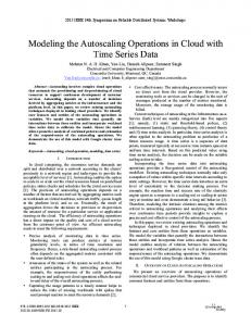
The following example changes the plot by using year and quarter value to label the tick marks. The FORMAT statement causes PROC GPLOT to use the YYQC format to print the date values. This example also shows how to place reference lines on the plot with the HREF= option. Reference lines are drawn to mark the boundary between years. proc gplot data=uscpi; symbol i=spline v=circle h=2; plot cpi * date / haxis= ’1jan89’d to ’1jul91’d by qtr href= ’1jan90’d to ’1jan91’d by year; format date yyqc6.; run;


65



Figure 2.8.


Overlay Plots of Different Variables You can plot two or more series on the same graph. Plot series stored in different variables by specifying multiple plot requests on one PLOT statement, and use the OVERLAY option. Specify a different SYMBOL statement for each plot. For example, the following statements plot the CPI, FORECAST, L95, and U95 variables produced by PROC ARIMA in a previous example. The SYMBOL1 statement is used for the actual series. Values of the actual series are labeled with a star, and the points are not connected. The SYMBOL2 statement is used for the forecast series. Values of the forecast series are labeled with an open circle, and the points are connected with a smooth curve. The SYMBOL3 statement is used for the upper and lower confidence limits series. Values of the upper and lower confidence limits points are not plotted, but a broken line is drawn between the points. A reference line is drawn to mark the start of the forecast period. Quarterly tick marks with YYQC format date values are used. proc arima data=uscpi; identify var=cpi(1); estimate q=1; forecast id=date interval=month lead=12 out=arimaout; run; proc gplot data=arimaout; symbol1 i=none v=star h=2; symbol2 i=spline v=circle h=2; symbol3 i=spline l=5; format date yyqc4.; plot cpi * date = 1 forecast * date = 2


66

Chapter 2. Plotting Time Series ( l95 u95 ) * date = 3 / overlay haxis= ’1jan89’d to ’1jul92’d by qtr href= ’15jul91’d ; run;


Figure 2.9.

Plot of ARIMA Forecast

Overlay Plots of Interleaved Series You can also plot several series on the same graph when the different series are stored in the same variable in interleaved form. Plot interleaved time series by using the values of the ID variable to distinguish the different series and by selecting different SYMBOL statements for each plot. The following example plots the output data set produced by PROC FORECAST in a previous example. Since the residual series has a different scale than the other series, it is excluded from the plot with a WHERE statement. The – TYPE– variable is used on the PLOT statement to identify the different series and to select the SYMBOL statements to use for each plot. The first SYMBOL statement is used for the first sorted value of – TYPE– , which is – TYPE– =ACTUAL. The second SYMBOL statement is used for the second sorted value of the – TYPE– variable (– TYPE– =FORECAST), and so forth. proc forecast data=uscpi interval=month lead=12 out=foreout outfull outresid; var cpi; id date;

67


Part 1. General Information run; proc gplot data=foreout; symbol1 i=none v=star h=2; symbol2 i=spline v=circle h=2; symbol3 i=spline l=20; symbol4 i=spline l=20; format date yyqc4.; plot cpi * date = _type_ / haxis= ’1jan89’d to ’1jul92’d by qtr href= ’15jul91’d ; where _type_ ^= ’RESIDUAL’; run;


Figure 2.10.

Plot of Forecast

Residual Plots The following example plots the residuals series that was excluded from the plot in the previous example. The SYMBOL statement specifies a needle plot, so that each residual point is plotted as a vertical line showing deviation from zero. proc gplot data=foreout; symbol1 i=needle v=circle width=6; format date yyqc4.; plot cpi * date / haxis= ’1jan89’d to ’1jul91’d by qtr ; where _type_ = ’RESIDUAL’; run;


68

Chapter 2. Plotting Time Series The plot is shown in Figure 2.11.

Figure 2.11.

Plot of Residuals

Using PROC PLOT The following statements use the PLOT procedure to plot CPI in the USCPI data set against DATE. (The data set plotted contains more observations than shown in the previous examples.) The plotting character used is a plus sign (+). proc plot data=uscpi; plot cpi * date = ’+’; run;


69



Plot of cpi*date.

Symbol used is ’+’.

cpi | 140 + | | | | | ++ + 135 + + + + + | + + | + | + | + | 130 + ++ | + + | + + | + | | + + + 125 + + + | + ++ | + | + | + | + 120 + | --+-----------+-----------+-----------+-----------+-----------+-----------+JUN1988 JAN1989 JUL1989 FEB1990 AUG1990 MAR1991 OCT1991 date

Figure 2.12.


Controlling the Time Axis: Tick Marks and Reference Lines In the preceding example, the spacing of values on the time axis looks a bit odd in that the dates do not match for each year. Because DATE is a SAS date variable, the PLOT procedure needs additional instruction on how to place the time axis tick marks. The following statements use the HAXIS= option to tell PROC PLOT to mark the axis at the start of each quarter. proc plot data=uscpi; plot cpi * date = ’+’ / haxis= ’1jan89’d to ’1jul91’d by qtr; run;



70


Plot of cpi*date.


140 + | | | | + + + 135 + + + + + | + + + cpi | + | + | 130 + + + | + + + | + | + | + + + 125 + + + | + + + | + | + + | + 120 + ---+------+------+------+------+------+------+------+------+------+------+-J A J O J A J O J A J A P U C A P U C A P U N R L T N R L T N R L 1 1 1 1 1 1 1 1 1 1 1 9 9 9 9 9 9 9 9 9 9 9 8 8 8 8 9 9 9 9 9 9 9 9 9 9 9 0 0 0 0 1 1 1 date

Figure 2.13.


The following example improves the plot by placing tick marks every year and adds quarterly reference lines to the plot using the HREF= option. The FORMAT statement tells PROC PLOT to print just the year part of the date values on the axis. The plot is shown in Figure 2.14. proc plot data=uscpi; plot cpi * date = ’+’ / haxis= ’1jan89’d to ’1jan92’d by year href= ’1apr89’d to ’1apr91’d by qtr ; format date year4.; run;

71



Plot of cpi*date.


cpi | | | | | | | | | | 140 + | | | | | | | | | | | | | | | | | | | | | | | | | | | | | | | | | | | | | | | | | | | | | | | | | | | | | | | | | | |+ ++ 135 + | | | | | | | + ++ + | | | | | | | | ++ | | | | | | | | | + | | | | | | | | | +| | | | | | | | | | + | | | | | | | | | | | | | 130 + | | | | | ++ | | | | | | | | ++ | | | | | | | | | ++ | | | | | | | | | + | | | | | | | | | | | | | | | | | | + ++ | | | | | | 125 + | | + +| | | | | | | | |+ ++ | | | | | | | | + | | | | | | | | | + | | | | | | | | | | + | | | | | | | | | | + | | | | | | | | | 120 + | | | | | | | | | | | | | | | | | | | ---+------------------+------------------+------------------+-1989 1990 1991 1992 date

Figure 2.14.


Marking the Subperiod of Points In the preceding example, it is a little hard to tell which month each point is, although the quarterly reference lines help some. The following example shows how to set the plotting symbol to the first letter of the month name. A DATA step first makes a copy of DATE and gives this variable PCHAR a MONNAME1. format. The variable PCHAR is used in the PLOT statement to supply the plotting character. This example also changes the plot by using quarterly tick marks and by using the YYQC format to print the date values. This example also changes the HREF= option to use annual reference lines. The plot is shown in Figure 2.15. data temp; set uscpi; pchar = date; format pchar monname1.; run; proc plot data=temp; plot cpi * date = pchar / haxis= ’1jan89’d to ’1jul91’d by qtr href= ’1jan90’d to ’1jan91’d by year; format date yyqc4.; run;


72


Plot of cpi*date.

Symbol is value of pchar.

cpi | | | 140 + | | | | | | | | | | | | | | | | | M J J 135 + | J F M A | | N D | | | O | | | S | | | A | | | | 130 + | J J | | | A M | | | F M | | J | | | | | O N D | | 125 + A S | | | M J J | | | A | | | M | | | F | | | J | | 120 + | | | | | ---+-----+-----+-----+-----+-----+-----+-----+-----+-----+-----+-89:1 89:2 89:3 89:4 90:1 90:2 90:3 90:4 91:1 91:2 91:3 date

Figure 2.15.


Overlay Plots of Different Variables Plot different series in different variables by specifying the different plot requests, each with its own plotting character, on the same PLOT statement, and use the OVERLAY option. For example, the following statements plot the CPI, FORECAST, L95, and U95 variables produced by PROC ARIMA in a previous example. The actual series CPI is labeled with the plot character plus (+). The forecast series is labeled with the plot character F. The upper and lower confidence limits are labeled with the plot character period (.). The plot is shown in Figure 2.16. proc arima data=uscpi; identify var=cpi(1); estimate q=1; forecast id=date interval=month lead=12 out=arimaout; run; proc plot data=arimaout; plot cpi * date = ’+’ forecast * date = ’F’ ( l95 u95 ) * date = ’.’ / overlay haxis= ’1jan89’d to ’1jul92’d by qtr href= ’1jan90’d to ’1jan92’d by year ; run;

73



Plot Plot Plot Plot

of of of of

cpi*date. FORECAST*date. L95*date. U95*date.

Symbol Symbol Symbol Symbol

used used used used

is is is is

’+’. ’F’. ’.’. ’.’.

cpi | | | | 150 + | | | | | | | | | | | | | | | . . . | | | | .. .F F F 140 + | | .. F FF F . . | | | . .F F FF . .. .. | | | F ++ + ++ F. . .. | | | + + ++ + .. | | | . + +. | | 130 + | .F + ++ F | | | + + ++ . | | | . .+ + + +F | | | ++ + + +. . | | | | ++ + F | | | 120 + . | | | | | | | ---+----+----+----+----+----+----+----+----+----+----+----+----+----+----+-J A J O J A J O J A J O J A J A P U C A P U C A P U C A P U N R L T N R L T N R L T N R L 1 1 1 1 1 1 1 1 1 1 1 1 1 1 1 9 9 9 9 9 9 9 9 9 9 9 9 9 9 9 8 8 8 8 9 9 9 9 9 9 9 9 9 9 9 9 9 9 9 0 0 0 0 1 1 1 1 2 2 2 date NOTE: 15 obs had missing values.

Figure 2.16.

77 obs hidden.

Plot of ARIMA Forecast

Overlay Plots of Interleaved Series Plot interleaved time series by using the first character of the ID variable to distinguish the different series as the plot character. The following example plots the output data set produced by PROC FORECAST in a previous example. The – TYPE– variable is used on the PLOT statement to supply plotting characters to label the different series. The actual series is plotted with A, the forecast series is plotted with F, the lower confidence limit is plotted with L, and the upper confidence limit is plotted with U. Since the residual series has a different scale than the other series, it is excluded from the plot with a WHERE statement. The plot is shown in Figure 2.17. proc forecast data=uscpi interval=month lead=12 out=foreout outfull outresid; var cpi; id date; run; proc plot data=foreout; plot cpi * date = _type_ / haxis= ’1jan89’d to ’1jul92’d by qtr


74

Chapter 2. Plotting Time Series href= ’1jan90’d to ’1jan92’d by year ; where _type_ ^= ’RESIDUAL’; run;

Plot of cpi*date.

Symbol is value of _TYPE_.

cpi | | | | 150 + | | | | | | | | | | | | | | | U | | | | UU F F | | | U UF FF L L 140 + | | U UF F FL L | | | UF F FL L | | | AA FL L | | | A A AA A | | | AA A A| | | | A F | | 130 + | F A AA | | | | A AA | | | A AA | | | F A AA A | | | | AA A | | | | AA A | | | 120 + | | | | | | | ---+----+----+----+----+----+----+----+----+----+----+----+----+----+----+-J A J O J A J O J A J O J A J A P U C A P U C A P U C A P U N R L T N R L T N R L T N R L 1 1 1 1 1 1 1 1 1 1 1 1 1 1 1 9 9 9 9 9 9 9 9 9 9 9 9 9 9 9 8 8 8 8 9 9 9 9 9 9 9 9 9 9 9 9 9 9 9 0 0 0 0 1 1 1 1 2 2 2 date NOTE: 36 obs hidden.

Figure 2.17.

Plot of Forecast

Residual Plots The following example plots the residual series that was excluded from the plot in the previous example. The VREF=0 option is used to draw a reference line at 0 on the vertical axis. The plot is shown in Figure 2.18. proc plot data=foreout; plot cpi * date = ’*’ / vref=0 haxis= ’1jan89’d to ’1jul91’d by qtr href= ’1jan90’d to ’1jan91’d by year ; where _type_ = ’RESIDUAL’; run;

75



Plot of cpi*date.

Symbol used is ’*’.

cpi | | | 1.0 + | | | | | | | | | | | | | * | | * * | 0.5 + | * | | | | | | * | * * | | | * | * | | | * * | 0.0 +-*--------------------*------+--*------------------------+---------------| * * | * | | * * | | * | | * | * * * | * * | * * | * | | | -0.5 + * | | * | | | --+------+------+------+------+------+------+------+------+------+------+-J A J O J A J O J A J A P U C A P U C A P U N R L T N R L T N R L 1 1 1 1 1 1 1 1 1 1 1 9 9 9 9 9 9 9 9 9 9 9 8 8 8 8 9 9 9 9 9 9 9 9 9 9 9 0 0 0 0 1 1 1 date

Figure 2.18.

Plot of Residuals

Using PROC TIMEPLOT The TIMEPLOT procedure plots time series data vertically on the page instead of horizontally across the page as the PLOT procedure does. PROC TIMEPLOT can also print the data values as well as plot them. The following statements use the TIMEPLOT procedure to plot CPI in the USCPI data set. Only the last 14 observations are included in this example. The plot is shown in Figure 2.19. proc timeplot data=uscpi; plot cpi; id date; where date >= ’1jun90’d; run;


76

Chapter 2. Calendar and Time Functions

date

cpi

JUN1990 JUL1990 AUG1990 SEP1990 OCT1990 NOV1990 DEC1990 JAN1991 FEB1991 MAR1991 APR1991 MAY1991 JUN1991 JUL1991

129.90 130.40 131.60 132.70 133.50 133.80 133.80 134.60 134.80 135.00 135.20 135.60 136.00 136.20

Figure 2.19.

min max 129.9 136.2 *-------------------------------------------------------* |c | | c | | c | | c | | c | | c | | c | | c | | c | | c | | c | | c | | c | | c| *-------------------------------------------------------*

Output Produced by PROC TIMEPLOT

The TIMEPLOT procedure has several interesting features not discussed here. Refer to "The TIMEPLOT Procedure" in the SAS Procedures Guide for more information.

Calendar and Time Functions Calendar and time functions convert calendar and time variables like YEAR, MONTH, DAY, and HOUR, MINUTE, SECOND into SAS date or datetime values, and vice versa. The SAS calendar and time functions are DATEJUL, DATEPART, DAY, DHMS, HMS, HOUR, JULDATE, MDY, MINUTE, MONTH, QTR, SECOND, TIMEPART, WEEKDAY, YEAR, and YYQ. Refer to SAS Language Reference for more details about these functions.

Computing Dates from Calendar Variables The MDY function converts MONTH, DAY, and YEAR values to a SAS date value. For example, MDY(10,17,91) returns the SAS date value ’17OCT91’D. The YYQ function computes the SAS date for the first day of a quarter. For example, YYQ(91,4) returns the SAS date value ’1OCT91’D. he DATEJUL function computes the SAS date for a Julian date. For example, DATEJUL(91290) returns the SAS date ’17OCT91’D. The YYQ and MDY functions are useful for creating SAS date variables when the ID values recorded in the data are year and quarter; year and month; or year, month, and day, instead of dates that can be read with a date informat. For example, the following statements read quarterly estimates of the gross national product of the U.S. from 1990:I to 1991:II from data records on which dates are coded as separate year and quarter values. The YYQ function is used to compute the variable DATE.

77


Part 1. General Information data usecon; input year qtr gnp; date = yyq( year, qtr ); format date yyqc.; datalines; 1990 1 5375.4 1990 2 5443.3 1990 3 5514.6 1990 4 5527.3 1991 1 5557.7 1991 2 5615.8 ;

The monthly USCPI data shown in a previous example contained time ID values represented in the MONYY format. If the data records instead contain separate year and month values, the data can be read in and the DATE variable computed with the following statements: data uscpi; input month year cpi; date = mdy( month, 1, year ); format date monyy.; datalines; 6 90 129.9 7 90 130.4 8 90 131.6 ... etc. ... ;

Computing Calendar Variables from Dates The functions YEAR, MONTH, DAY, WEEKDAY, and JULDATE compute calendar variables from SAS date values. Returning to the example of reading the USCPI data from records containing date values represented in the MONYY format, you can find the month and year of each observation from the SAS dates of the observations using the following statements. data uscpi; input date monyy7. cpi; format date monyy7.; year = year( date ); month = month( date ); datalines; jun1990 129.9 jul1990 130.4 aug1990 131.6 sep1990 132.7 ... etc. ... ;


78

Chapter 2. Calendar and Time Functions

Converting between Date, Datetime, and Time Values The DATEPART function computes the SAS date value for the date part of a SAS datetime value. The TIMEPART function computes the SAS time value for the time part of a SAS datetime value. The HMS function computes SAS time values from HOUR, MINUTE, and SECOND time variables. The DHMS function computes a SAS datetime value from a SAS date value and HOUR, MINUTE, and SECOND time variables. See the “Date, Time, and Datetime Functions” section on page 125 for more information on the sytax of these functions.

Computing Datetime Values To compute datetime ID values from calendar and time variables, first compute the date and then compute the datetime with DHMS. For example, suppose you read tri-hourly temperature data with time recorded as YEAR, MONTH, DAY, and HOUR. The following statements show how to compute the ID variable DATETIME: data weather; input year month day hour temp; datetime = dhms( mdy( month, day, year ), hour, 0, 0 ); format datetime datetime10.; datalines; 91 10 16 21 61 91 10 17 0 56 91 10 17 3 53 91 10 17 6 54 91 10 17 9 65 91 10 17 12 72 ... etc. ... ;

Computing Calendar and Time Variables The functions HOUR, MINUTE, and SECOND compute time variables from SAS datetime values. The DATEPART function and the date-to-calendar variables functions can be combined to compute calendar variables from datetime values. For example, suppose the date and time of the tri-hourly temperature data in the preceding example were recorded as datetime values in the datetime format. The following statements show how to compute the YEAR, MONTH, DAY, and HOUR of each observation and include these variables in the SAS data set: data weather; input datetime datetime13. temp; format datetime datetime10.; hour = hour( datetime );

79


Part 1. General Information date = datepart( datetime ); year = year( date ); month = month( date ); day = day( date ); datalines; 16oct91:21:00 61 17oct91:00:00 56 17oct91:03:00 53 17oct91:06:00 54 17oct91:09:00 65 17oct91:12:00 72 ... etc. ... ;

Interval Functions INTNX and INTCK The SAS interval functions INTNX and INTCK perform calculations with date, datetime values, and time intervals. They can be used for calendar calculations with SAS date values, to count time intervals between dates, and to increment dates or datetime values by intervals. The INTNX function increments dates by intervals. INTNX computes the date or datetime of the start of the interval a specified number of intervals from the interval containing a given date or datetime value.


80

Chapter 2. Interval Functions INTNX and INTCK The form of the INTNX function is INTNX( interval, from, n ) where: interval

is a character constant or variable containing an interval name.

from

is a SAS date value (for date intervals) or datetime value (for datetime intervals).

n

is the number of intervals to increment from the interval containing the from value.

alignment

controls the alignment of SAS dates, within the interval, used to identify output observations. Can take the values BEGINNING|B, MIDDLE|M, or END|E.

The number of intervals to increment, n, can be positive, negative, or zero. For example, the statement NEXTMON = INTNX(’MONTH’,DATE,1); assigns to the variable NEXTMON the date of the first day of the month following the month containing the value of DATE. The INTCK function counts the number of interval boundaries between two dates or between two datetime values. The form of the INTCK function is INTCK( interval, from, to ) where: interval

is a character constant or variable containing an interval name

from

is the starting date (for date intervals) or datetime value (for datetime intervals)

to

is the ending date (for date intervals) or datetime value (for datetime intervals).

For example, the statement NEWYEARS = INTCK(’YEAR’,DATE1,DATE2); assigns to the variable NEWYEARS the number of New Year’s Days between the two dates.

Incrementing Dates by Intervals Use the INTNX function to increment dates by intervals. For example, suppose you want to know the date of the start of the week that is six weeks from the week of 17 October 1991. The function INTNX(’WEEK’,’17OCT91’D,6) returns the SAS date value ’24NOV1991’D. One practical use of the INTNX function is to generate periodic date values. For example, suppose the monthly U.S. Consumer Price Index data in a previous example were recorded without any time identifier on the data records. Given that you

81


Part 1. General Information know the first observation is for June 1990, the following statements use the INTNX function to compute the ID variable DATE for each observation: data uscpi; input cpi; date = intnx( ’month’, ’1jun1990’d, _n_-1 ); format date monyy7.; datalines; 129.9 130.4 131.6 132.7 ... etc. ... ;

The automatic variable – N– counts the number of times the DATA step program has executed, and in this case – N– contains the observation number. Thus – N– -1 is the increment needed from the first observation date. Alternatively, we could increment from the month before the first observation, in which case the INTNX function in this example would be written INTNX(’MONTH’,’1MAY1990’D,– N– ).


82

Chapter 2. Interval Functions INTNX and INTCK

Alignment of SAS Dates Any date within the time interval corresponding to an observation of a periodic time series can serve as an ID value for the observation. For example, the USCPI data in a previous example might have been recorded with dates at the 15th of each month. The person recording the data might reason that since the CPI values are monthly averages, midpoints of the months might be the appropriate ID values. However, as far as SAS/ETS procedures are concerned, what is important about monthly data is the month of each observation, not the exact date of the ID value. If you indicate that the data are monthly (with an INTERVAL=MONTH) option, SAS/ETS procedures ignore the day of the month in processing the ID variable. The MONYY format also ignores the day of the month. Thus, you could read in the monthly USCPI data with midmonth DATE values using the following statements: data uscpi; input date date9. cpi; format date monyy7.; datalines; 15jun1990 129.9 15jul1990 130.4 15aug1990 131.6 15sep1990 132.7 ... etc. ... ;

The results of using this version of the USCPI data set for analysis with SAS/ETS procedures would be the same as with first-of-month values for DATE. Although you can use any date within the interval as an ID value for the interval, you may find working with time series in SAS less confusing if you always use date ID values normalized to the start of the interval. For some applications it may be preferable to use end of period dates, such as 31Jan1994, 28Feb1994, 31Mar1994, ..., 31Dec1994. For other applications, such as plotting time series, it may be more convenient to use interval midpoint dates to identify the observations. SAS/ETS procedures provide an ALIGN= option to control the alignment of dates for output time series observations. Procedures supporting the ALIGN= option are ARIMA, DATASOURCE, EXPAND, and FORECAST. In addition, the INTNX library function supports an optional argument to specify the alignment of the returned date value. To normalize date values to the start of intervals, use the INTNX function with a 0 increment. The INTNX function with an increment of 0 computes the date of the first day of the interval (or the first second of the interval for datetime values). For example, INTNX(’MONTH’,’17OCT1991’D,0, ’1OCT1991’D’.

83

BEG) returns the date


Part 1. General Information The following statements show how the preceding example can be changed to normalize the mid-month DATE values to first-of-month and end-of-month values. For exposition, the first-of-month value is transformed back into a middle-of-month value. data uscpi; input date date9. cpi; format date monyy7.; monthbeg = intnx( ’month’, date, 0, beg ); midmonth = intnx( ’month’, monthbeg, 0, mid ); monthend = intnx( ’month’, date, 0, end ); datalines; 15jun1990 129.9 15jul1990 130.4 15aug1990 131.6 15sep1990 132.7 ... etc. ... ;

If you want to compute the date of a particular day within an interval, you can use calendar functions, or you can increment the starting date of the interval by a number of days. The following example shows three ways to compute the 7th day of the month: data test; set uscpi; mon07_1 = mdy( month(date), 7, year(date) ); mon07_2 = intnx( ’month’, date, 0, beg ) + 6; mon07_3 = intnx( ’day’, date, 6 ); run;

Computing the Width of a Time Interval To compute the width of a time interval, subtract the ID value of the start of the next interval from the ID value of the start of the current interval. If the ID values are SAS dates, the width will be in days. If the ID values are SAS datetime values, the width will be in seconds. For example, the following statements show how to add a variable WIDTH to the USCPI data set that contains the number of days in the month for each observation: data uscpi; input date date9. cpi; format date monyy7.; width = intnx( ’month’, date, 1 ) - intnx( ’month’, date, 0 ); datalines; 15jun1990 129.9 15jul1990 130.4 15aug1990 131.6 15sep1990 132.7 ... etc. ... ;


84

Chapter 2. Interval Functions INTNX and INTCK

Computing the Ceiling of an Interval To shift a date to the start of the next interval if not already at the start of an interval, subtract 1 from the date and use INTNX to increment the date by 1 interval. For example, the following statements add the variable NEWYEAR to the monthly USCPI data set. The variable NEWYEAR contains the date of the next New Year’s Day. NEWYEAR contains the same value as DATE when the DATE value is the start of year and otherwise contains the date of the start of the next year. data test; set uscpi; newyear = intnx( ’year’, date - 1, 1 ); format newyear date.; run;

Counting Time Intervals Use the INTCK function to count the number of interval boundaries between two dates. Note that the INTCK function counts the number of times the beginning of an interval is reached in moving from the first date to the second. It does not count the number of complete intervals between two dates. For example, the function INTCK(’MONTH’,’1JAN1991’D,’31JAN1991’D) returns 0, since the two dates are within the same month. The function INTCK(’MONTH’,’31JAN1991’D,’1FEB1991’D) returns 1, since the two dates lie in different months that are one month apart. When the first date is later than the second date, INTCK returns a negative count. For example, the function INTCK(’MONTH’,’1FEB1991’D,’31JAN1991’D) returns -1. The following example shows how to use the INTCK function to count the number of Sundays, Mondays, Tuesdays, and so forth, in each month. The variables NSUNDAY, NMONDAY, NTUESDAY, and so forth, are added to the USCPI data set. data uscpi; set uscpi; d0 = intnx( ’month’, date, 0 ) - 1; d1 = intnx( ’month’, date, 1 ) - 1; nsunday = intck( ’week.1’, d0, d1 ); nmonday = intck( ’week.2’, d0, d1 ); ntuesday = intck( ’week.3’, d0, d1 ); nwedday = intck( ’week.4’, d0, d1 ); nthurday = intck( ’week.5’, d0, d1 ); nfriday = intck( ’week.6’, d0, d1 ); nsatday = intck( ’week.7’, d0, d1 ); drop d0 d1; run;

85


Part 1. General Information Since the INTCK function counts the number of interval beginning dates between two dates, the number of Sundays is computed by counting the number of week boundaries between the last day of the previous month and the last day of the current month. To count Mondays, Tuesdays, and so forth, shifted week intervals are used. The interval type WEEK.2 specifies weekly intervals starting on Mondays, WEEK.3 specifies weeks starting on Tuesdays, and so forth.

Checking Data Periodicity Suppose you have a time series data set, and you want to verify that the data periodicity is correct, the observations are dated correctly, and the data set is sorted by date. You can use the INTCK function to compare the date of the current observation with the date of the previous observation and verify that the dates fall into consecutive time intervals. For example, the following statements verify that the data set USCPI is a correctly dated monthly data set. The RETAIN statement is used to hold the date of the previous observation, and the automatic variable – N– is used to start the verification process with the second observation. data _null_; set uscpi; retain prevdate; if _n_ > 1 then if intck( ’month’, prevdate, date ) ^= 1 then put "Bad date sequence at observation number " _n_; prevdate = date; run;

Filling in Omitted Observations in a Time Series Data Set Recall that most SAS/ETS procedures expect input data to be in the standard form, with no omitted observations in the sequence of time periods. When data are missing for a time period, the data set should contain a missing observation, in which all variables except the ID variables have missing values. You can replace omitted observations in a time series data set with missing observations by merging the data set with a data set containing a complete sequence of dates. The following statements create a monthly data set, OMITTED, from data lines containing records for an intermittent sample of months. (Data values are not shown.) This data set is converted to a standard form time series data set in four steps. First, the OMITTED data set is sorted to make sure it is in time order. Second, the first and last date in the data set are determined and stored in the data set RANGE. Third, the data set DATES is created containing only the variable DATE and containing monthly observations for the needed time span. Finally, the data sets OMITTED and DATES are merged to produce a standard form time series data set with missing observations inserted for the omitted records.


86

Chapter 2. Interval Functions INTNX and INTCK data omitted; input date monyy7. x y z; format date monyy7.; datalines; jan1991 ... mar1991 ... apr1991 ... jun1991 ... ... etc. ... ; proc sort data=omitted; by date; run; data range; retain from to; set omitted end=lastobs; if _n_ = 1 then from = date; if lastobs then do; to = date; output; end; run; data dates; set range; date = from; do while( date = ’1jan1991’d; cpilag = lag( cpi ); /* WRONG PLACEMENT! */ run;

If the subsetting IF statement comes before the LAG function call, the value of CPILAG will be missing for January 1991, even though a value for December 1990 is available in the USCPI data set. To avoid losing this value, you must rearrange the statements to ensure that the LAG function is actually executed for the December 1990 observation. data subset; set uscpi; cpilag = lag( cpi ); if date >= ’1jan1991’d; run;

In other cases, the subsetting statement should come before the LAG and DIF functions. For example, the following statements subset the FOREOUT data set shown in a previous example to select only – TYPE– =RESIDUAL observations and also to compute the variable LAGRESID. data residual; set foreout; if _type_ = "RESIDUAL"; lagresid = lag( cpi ); run;

Another pitfall of LAG and DIF functions arises when they are used to process time series cross-sectional data sets. For example, suppose you want to add the variable CPILAG to the CPICITY data set shown in a previous example. You might use the following statements: data cpicity; set cpicity; cpilag = lag( cpi ); run;

However, these statements do not yield the desired result. In the data set produced by these statements, the value of CPILAG for the first observation for the first city is missing (as it should be), but in the first observation for all later cities, CPILAG contains the last value for the previous city. To correct this, set the lagged variable to missing at the start of each cross section, as follows. SAS OnlineDoc: Version 8

90

Chapter 2. Lags, Leads, Differences, and Summations data cpicity; set cpicity; by city date; cpilag = lag( cpi ); if first.city then cpilag = .; run;

Alternatives to LAG and DIF Functions You can also calculate lags and differences in the DATA step without using LAG and DIF functions. For example, the following statements add the variables CPILAG and CPIDIF to the USCPI data set: data uscpi; set uscpi; retain cpilag; cpidif = cpi - cpilag; output; cpilag = cpi; run;

The RETAIN statement prevents the DATA step from reinitializing CPILAG to a missing value at the start of each iteration and thus allows CPILAG to retain the value of CPI assigned to it in the last statement. The OUTPUT statement causes the output observation to contain values of the variables before CPILAG is reassigned the current value of CPI in the last statement. This is the approach that must be used if you want to build a variable that is a function of its previous lags. You can also use the EXPAND procedure to compute lags and differences. For example, the following statements compute lag and difference variables for CPI: proc expand data=uscpi out=uscpi method=none; id date; convert cpi=cpilag / transform=( lag 1 ); convert cpi=cpidif / transform=( dif 1 ); run;

LAG and DIF Functions in PROC MODEL The preceding discussion of LAG and DIF functions applies to LAG and DIF functions available in the DATA step. However, LAG and DIF functions are also used in the MODEL procedure. The MODEL procedure LAG and DIF functions do not work like the DATA step LAG and DIF functions. The LAG and DIF functions supported by PROC MODEL are true lag and difference functions, not queuing functions. Unlike the DATA step, the MODEL procedure processes observations from a single input data set, so the "previous observation" is always clearly defined in a PROC MODEL program. Therefore, PROC MODEL is able to define LAG and DIF as true lagging functions that operate on values from the previous observation. See Chapter 14, “The MODEL Procedure,” for more information on LAG and DIF functions in the MODEL procedure.

91



Multiperiod Lags and Higher-Order Differencing To compute lags at a lagging period greater than 1, add the lag length to the end of the LAG keyword to specify the lagging function needed. For example, the LAG2 function returns the value of its argument two calls ago, the LAG3 function returns the value of its argument three calls ago, and so forth. To compute differences at a lagging period greater than 1, add the lag length to the end of the DIF keyword. For example, the DIF2 function computes the differences between the value of its argument and the value of its argument two calls ago. (The maximum lagging period is 100.) The following statements add the variables CPILAG12 and CPIDIF12 to the USCPI data set. CPILAG12 contains the value of CPI from the same month one year ago. CPIDIF12 contains the change in CPI from the same month one year ago. (In this case, the first 12 values of CPILAG12 and CPIDIF12 will be missing.) data uscpi; set uscpi; cpilag12 = lag12( cpi ); cpidif12 = dif12( cpi ); run;

To compute second differences, take the difference of the difference. To compute higher-order differences, nest DIF functions to the order needed. For example, the following statements compute the second difference of CPI: data uscpi; set uscpi; cpi2dif = dif( dif( cpi ) ); run;

Multiperiod lags and higher-order differencing can be combined. For example, the following statements compute monthly changes in the inflation rate, with inflation rate computed as percent change in CPI from the same month one year ago: data uscpi; set uscpi; infchng = dif( 100 * dif12( cpi ) / lag12( cpi ) ); run;

Percent Change Calculations There are several common ways to compute the percent change in a time series. This section illustrates the use of LAG and DIF functions by showing SAS statements for various kinds of percent change calculations.

Computing Period-to-Period Change To compute percent change from the previous period, divide the difference of the series by the lagged value of the series and multiply by 100. SAS OnlineDoc: Version 8

92

Chapter 2. Lags, Leads, Differences, and Summations data uscpi; set uscpi; pctchng = dif( cpi ) / lag( cpi ) * 100; label pctchng = "Monthly Percent Change, At Monthly Rates"; run;

Often, changes from the previous period are expressed at annual rates. This is done by exponentiation of the current-to-previous period ratio to the number of periods in a year and expressing the result as a percent change. For example, the following statements compute the month-over-month change in CPI as a percent change at annual rates: data uscpi; set uscpi; pctchng = ( ( cpi / lag( cpi ) ) ** 12 - 1 ) * 100; label pctchng = "Monthly Percent Change, At Annual Rates"; run;

Computing Year-over-Year Change To compute percent change from the same period in the previous year, use LAG and DIF functions with a lagging period equal to the number of periods in a year. (For quarterly data, use LAG4 and DIF4. For monthly data, use LAG12 and DIF12.) For example, the following statements compute monthly percent change in CPI from the same month one year ago: data uscpi; set uscpi; pctchng = dif12( cpi ) / lag12( cpi ) * 100; label pctchng = "Percent Change from One Year Ago"; run;

To compute year-over-year percent change measured at a given period within the year, subset the series of percent changes from the same period in the previous year to form a yearly data set. Use an IF or WHERE statement to select observations for the period within each year on which the year-over-year changes are based. For example, the following statements compute year-over-year percent change in CPI from December of the previous year to December of the current year: data annual; set uscpi; pctchng = dif12( cpi ) / lag12( cpi ) * 100; label pctchng = "Percent Change: December to December"; if month( date ) = 12; format date year4.; run;

Computing Percent Change in Yearly Averages To compute changes in yearly averages, first aggregate the series to an annual series using the EXPAND procedure, and then compute the percent change of the annual 93


Part 1. General Information series. (See Chapter 11, “The EXPAND Procedure,” for more information on PROC EXPAND.) For example, the following statements compute percent changes in the annual averages of CPI: proc expand data=uscpi out=annual from=month to=year; convert cpi / observed=average method=aggregate; run; data annual; set annual; pctchng = dif( cpi ) / lag( cpi ) * 100; label pctchng = "Percent Change in Yearly Averages"; run;

It is also possible to compute percent change in the average over the most recent yearly span. For example, the following statements compute monthly percent change in the average of CPI over the most recent 12 months from the average over the previous 12 months: data uscpi; retain sum12 0; drop sum12 ave12 cpilag12; set uscpi; sum12 = sum12 + cpi; cpilag12 = lag12( cpi ); if cpilag12 ^= . then sum12 = sum12 - cpilag12; if lag11( cpi ) ^= . then ave12 = sum12 / 12; pctchng = dif12( ave12 ) / lag12( ave12 ) * 100; label pctchng = "Percent Change in 12 Month Moving Ave."; run;

This example is a complex use of LAG and DIF functions that requires care in handling the initialization of the moving-window averaging process. The LAG12 of CPI is checked for missing values to determine when more than 12 values have been accumulated, and older values must be removed from the moving sum. The LAG11 of CPI is checked for missing values to determine when at least 12 values have been accumulated; AVE12 will be missing when LAG11 of CPI is missing. The DROP statement prevents temporary variables from being added to the data set. Note that the DIF and LAG functions must execute for every observation or the queues of remembered values will not operate correctly. The CPILAG12 calculation must be separate from the IF statement. The PCTCHNG calculation must not be conditional on the IF statement. The EXPAND procedure provides an alternative way to compute moving averages.

Leading Series Although the SAS System does not provide a function to look ahead at the "next" value of a series, there are a couple of ways to perform this task. SAS OnlineDoc: Version 8

94

Chapter 2. Lags, Leads, Differences, and Summations The most direct way to compute leads is to use the EXPAND procedure. For example proc expand data=uscpi out=uscpi method=none; id date; convert cpi=cpilead1 / transform=( lead 1 ); convert cpi=cpilead2 / transform=( lead 2 ); run;

Another way to compute lead series in SAS software is by lagging the time ID variable, renaming the series, and merging the result data set back with the original data set. For example, the following statements add the variable CPILEAD to the USCPI data set. The variable CPILEAD contains the value of CPI in the following month. (The value of CPILEAD will be missing for the last observation, of course.) data temp; set uscpi; keep date cpi; rename cpi = cpilead; date = lag( date ); if date ^= .; run; data uscpi; merge uscpi temp; by date; run;

To compute leads at different lead lengths, you must create one temporary data set for each lead length. For example, the following statements compute CPILEAD1 and CPILEAD2, which contain leads of CPI for 1 and 2 periods, respectively: data temp1(rename=(cpi=cpilead1)) temp2(rename=(cpi=cpilead2)); set uscpi; keep date cpi; date = lag( date ); if date ^= . then output temp1; date = lag( date ); if date ^= . then output temp2; run; data uscpi; merge uscpi temp1 temp2; by date; run;

Summing Series Simple cumulative sums are easy to compute using SAS sum statements. The following statements show how to compute the running sum of variable X in data set A, adding XSUM to the data set.

95


Part 1. General Information data a; set a; xsum + x; run;

The SAS sum statement automatically retains the variable XSUM and initializes it to 0, and the sum statement treats missing values as 0. The sum statement is equivalent to using a RETAIN statement and the SUM function. The previous example could also be written as follows: data a; set a; retain xsum; xsum = sum( xsum, x ); run;

You can also use the EXPAND procedure to compute summations. For example proc expand data=a out=a method=none; convert x=xsum / transform=( sum ); run;

Like differencing, summation can be done at different lags and can be repeated to produce higher-order sums. To compute sums over observations separated by lags greater than 1, use the LAG and SUM functions together, and use a RETAIN statement that initializes the summation variable to zero. For example, the following statements add the variable XSUM2 to data set A. XSUM2 contains the sum of every other observation, with even-numbered observations containing a cumulative sum of values of X from even observations, and odd-numbered observations containing a cumulative sum of values of X from odd observations. data a; set a; retain xsum2 0; xsum2 = sum( lag( xsum2 ), x ); run;

Assuming that A is a quarterly data set, the following statements compute running sums of X for each quarter. XSUM4 contains the cumulative sum of X for all observations for the same quarter as the current quarter. Thus, for a first-quarter observation, XSUM4 contains a cumulative sum of current and past first-quarter values. data a; set a; retain xsum4 0; xsum4 = sum( lag3( xsum4 ), x ); run;


96

Chapter 2. Transforming Time Series To compute higher-order sums, repeat the preceding process and sum the summation variable. For example, the following statements compute the first and second summations of X: data a; set a; xsum + x; x2sum + xsum; run;

The following statements compute the second order four-period sum of X: data a; set a; retain xsum4 x2sum4 0; xsum4 = sum( lag3( xsum4 ), x ); x2sum4 = sum( lag3( x2sum4 ), xsum4 ); run;

You can also use PROC EXPAND to compute cumulative statistics and moving window statistics. See Chapter 11, “The EXPAND Procedure,” for details.

Transforming Time Series It is often useful to transform time series for analysis or forecasting. Many time series analysis and forecasting methods are most appropriate for time series with an unrestricted range, linear trend, and constant variance. Series that do not conform to these assumptions can often be transformed to series for which the methods are appropriate. Transformations can be useful for the following: range restrictions. Many time series cannot have negative values or may be limited by a maximum possible value. You can often create a transformed series with an unbounded range. nonlinear trends. Many economic time series grow exponentially. Exponential growth corresponds to linear growth in the logarithms of the series. series variability that changes over time. Various transformations can be used to stabilize the variance. non-stationarity. The %DFTEST macro can be used to test a series for nonstationarity which may then be removed by differencing.

97



Log Transformation The logarithmic transformation is often useful for series that must be greater than zero and that grow exponentially. For example, Figure 2.21 shows a plot of an airline passenger miles series. Notice that the series has exponential growth and the variability of the series increases over time. Airline passerger miles must also be zero or greater.

Figure 2.21.

Airline Series

The following statements compute the logarithms of the airline series: data a; set a; logair = log( air ); run;

Figure 2.22 shows a plot of the log transformed airline series. Notice that the log series has a linear trend and constant variance.


98

Chapter 2. Transforming Time Series

Figure 2.22.

Log Airline Series

The %LOGTEST macro can help you decide if a log transformation is appropriate for a series. See Chapter 4, “SAS Macros and Functions,” for more information on the %LOGTEST macro.

Other Transformations The Box-Cox transformation is a general class of transformations that includes the logarithm as a special case. The %BOXCOXAR macro can be used to find an optimal Box-Cox transformation for a time series. See Chapter 4 for more information on the %BOXCOXAR macro. The logistic transformation is useful for variables with both an upper and a lower bound, such as market shares. The logistic transformation is useful for proportions, percent values, relative frequencies, or probabilities. The logistic function transforms values between 0 and 1 to values that can range from -1 to +1. For example, the following statements transform the variable SHARE from percent values to an unbounded range: data a; set a; lshare = log( share / ( 100 - share ) ); run;

Many other data transformation can be used. You can create virtually any desired data transformation using DATA step statements.

99



The EXPAND Procedure and Data Transformations The EXPAND procedure provides a convenient way to transform series. For example, the following statements add variables for the logarithm of AIR and the logistic of SHARE to data set A: proc expand data=a out=a method=none; convert air=logair / transform=( log ); convert share=lshare / transform=( / 100 logit ); run;

See Table 11.1 in Chapter 11 for a complete list of transformations supported by PROC EXPAND.

Manipulating Time Series Data Sets This section discusses merging, splitting, and transposing time series data sets and interpolating time series data to a higher or lower sampling frequency.

Splitting and Merging Data Sets In some cases, you may want to separate several time series contained in one data set into different data sets. In other cases, you may want to combine time series from different data sets into one data set. To split a time series data set into two or more data sets containing subsets of the series, use a DATA step to create the new data sets and use the KEEP= data set option to control which series are included in each new data set. The following statements split the USPRICE data set shown in a previous example into two data sets, USCPI and USPPI: data uscpi(keep=date cpi) usppi(keep=date ppi); set usprice; run;

If the series have different time ranges, you can subset the time ranges of the output data sets accordingly. For example, if you know that CPI in USPRICE has the range August 1990 through the end of the data set, while PPI has the range from the beginning of the data set through June 1991, you could write the previous example as follows: data uscpi(keep=date cpi) usppi(keep=date ppi); set usprice; if date >= ’1aug1990’d then output uscpi; if date ’1may1991’d & date < ’1oct1991’d; run; proc transpose data=foreout out=trans(drop=_name_ _label_); var cpi; id _type_; by date; where date > ’1may1991’d & date < ’1oct1991’d; run; title "Transposed Data Set"; proc print data=trans; run;

The TRANSPOSE procedure adds the variables – NAME– and – LABEL– to the output data set. These variables contain the names and labels of the variables that were transposed. In this example, there is only one transposed variable, so – NAME– has the value CPI for all observations. Thus, – NAME– and – LABEL– are of no interest

101


Part 1. General Information and are dropped from the output data set using the DROP= data set option. (If none of the variables transposed have a label, PROC TRANSPOSE does not output the – LABEL– variable and the DROP=– LABEL– option produces a warning message. You can ignore this message, or you can prevent the message by omitting – LABEL– from the DROP= list.) The original and transposed data sets are shown in Figure 2.23. (The observation numbers shown for the original data set reflect the operation of the WHERE statement.) Original Data Set Obs

date

37 38 39 40 41 42 43 44 45 46 47 48

JUN1991 JUN1991 JUN1991 JUL1991 JUL1991 JUL1991 AUG1991 AUG1991 AUG1991 SEP1991 SEP1991 SEP1991

_TYPE_ ACTUAL FORECAST RESIDUAL ACTUAL FORECAST RESIDUAL FORECAST L95 U95 FORECAST L95 U95

_LEAD_ 0 0 0 0 0 0 1 1 1 2 2 2

cpi 136.000 136.146 -0.146 136.200 136.566 -0.366 136.856 135.723 137.990 137.443 136.126 138.761

Transposed Data Set Obs 1 2 3 4

date

ACTUAL

FORECAST

RESIDUAL

L95

U95

JUN1991 JUL1991 AUG1991 SEP1991

136.0 136.2 . .

136.146 136.566 136.856 137.443

-0.14616 -0.36635 . .

. . 135.723 136.126

. . 137.990 138.761

Figure 2.23.

Original and Transposed Data Sets

Transposing Cross-sectional Dimensions The following statements transpose the variable CPI in the CPICITY data set shown in a previous example from time series cross-sectional form to a standard form time series data set. (Only a subset of the data shown in the previous example is used here.) Note that the method shown in this example only works for a single variable. title "Original Data Set"; proc print data=cpicity; run; proc sort data=cpicity out=temp; by date city; run;


102

Chapter 2. Manipulating Time Series Data Sets proc transpose data=temp out=citycpi(drop=_name_ _label_); var cpi; id city; by date; run; title "Transposed Data Set"; proc print data=citycpi; run;

The names of the variables in the transposed data sets are taken from the city names in the ID variable CITY. The original and the transposed data sets are shown in Figure 2.24. Original Data Set Obs 1 2 3 4 5 6 7 8 9 10 11 12 13 14 15 16 17 18 19 20 21

city

date

cpi

Chicago Chicago Chicago Chicago Chicago Chicago Chicago Los Angeles Los Angeles Los Angeles Los Angeles Los Angeles Los Angeles Los Angeles New York New York New York New York New York New York New York

JAN90 FEB90 MAR90 APR90 MAY90 JUN90 JUL90 JAN90 FEB90 MAR90 APR90 MAY90 JUN90 JUL90 JAN90 FEB90 MAR90 APR90 MAY90 JUN90 JUL90

128.1 129.2 129.5 130.4 130.4 131.7 132.0 132.1 133.6 134.5 134.2 134.6 135.0 135.6 135.1 135.3 136.6 137.3 137.2 137.1 138.4

Transposed Data Set

Obs 1 2 3 4 5 6 7

Figure 2.24.

date JAN90 FEB90 MAR90 APR90 MAY90 JUN90 JUL90

Chicago

Los_ Angeles

128.1 129.2 129.5 130.4 130.4 131.7 132.0

132.1 133.6 134.5 134.2 134.6 135.0 135.6

New_York 135.1 135.3 136.6 137.3 137.2 137.1 138.4

Original and Transposed Data Sets

The following statements transpose the CITYCPI data set back to the original form of the CPICITY data set. The variable – NAME– is added to the data set to tell PROC TRANSPOSE the name of the variable in which to store the observations in the transposed data set. (If the (DROP=– NAME– – LABEL– ) option were omitted from

103


Part 1. General Information the first PROC TRANSPOSE step, this would not be necessary. PROC TRANSPOSE assumes ID – NAME– by default.) The NAME=CITY option in the PROC TRANSPOSE statement causes PROC TRANSPOSE to store the names of the transposed variables in the variable CITY. Because PROC TRANSPOSE recodes the values of the CITY variable to create valid SAS variable names in the transposed data set, the values of the variable CITY in the retransposed data set are not the same as the original. The retransposed data set is shown in Figure 2.25. data temp; set citycpi; _name_ = ’CPI’; run; proc transpose data=temp out=retrans name=city; by date; run; proc sort data=retrans; by city date; run; title "Retransposed Data Set"; proc print data=retrans; run;

Retransposed Data Set Obs 1 2 3 4 5 6 7 8 9 10 11 12 13 14 15 16 17 18 19 20 21

Figure 2.25.


date

city

JAN90 FEB90 MAR90 APR90 MAY90 JUN90 JUL90 JAN90 FEB90 MAR90 APR90 MAY90 JUN90 JUL90 JAN90 FEB90 MAR90 APR90 MAY90 JUN90 JUL90

Chicago Chicago Chicago Chicago Chicago Chicago Chicago Los_Angeles Los_Angeles Los_Angeles Los_Angeles Los_Angeles Los_Angeles Los_Angeles New_York New_York New_York New_York New_York New_York New_York

CPI 128.1 129.2 129.5 130.4 130.4 131.7 132.0 132.1 133.6 134.5 134.2 134.6 135.0 135.6 135.1 135.3 136.6 137.3 137.2 137.1 138.4

Data Set Transposed Back to Original Form

104

Chapter 2. Time Series Interpolation

Time Series Interpolation The EXPAND procedure interpolates time series. This section provides a brief summary of the use of PROC EXPAND for different kinds of time series interpolation problems. Most of the issues discussed in this section are explained in greater detail in Chapter 11. By default, the EXPAND procedure performs interpolation by first fitting cubic spline curves to the available data and then computing needed interpolating values from the fitted spline curves. Other interpolation methods can be requested. Note that interpolating values of a time series does not add any real information to the data as the interpolation process is not the same process that generated the other (nonmissing) values in the series. While time series interpolation can sometimes be useful, great care is needed in analyzing time series containing interpolated values.

Interpolating Missing Values To use the EXPAND procedure to interpolate missing values in a time series, specify the input and output data sets on the PROC EXPAND statement, and specify the time ID variable in an ID statement. For example, the following statements cause PROC EXPAND to interpolate values for missing values of all numeric variables in the data set USPRICE: proc expand data=usprice out=interpl; id date; run;

Interpolated values are computed only for embedded missing values in the input time series. Missing values before or after the range of a series are ignored by the EXPAND procedure. In the preceding example, PROC EXPAND assumes that all series are measured at points in time given by the value of the ID variable. In fact, the series in the USPRICE data set are monthly averages. PROC EXPAND may produce a better interpolation if this is taken into account. The following example uses the FROM=MONTH option to tell PROC EXPAND that the series is monthly and uses the CONVERT statement with the OBSERVED=AVERAGE to specify that the series values are averages over each month: proc expand data=usprice out=interpl from=month; id date; convert cpi ppi / observed=average; run;

105



Interpolating to a Higher or Lower Frequency You can use PROC EXPAND to interpolate values of time series at a higher or lower sampling frequency than the input time series. To change the periodicity of time series, specify the time interval of the input data set with the FROM= option, and specify the time interval for the desired output frequency with the TO= option. For example, the following statements compute interpolated weekly values of the monthly CPI and PPI series: proc expand data=usprice out=interpl from=month to=week; id date; convert cpi ppi / observed=average; run;

Interpolating between Stocks and Flows, Levels and Rates A distinction is made between variables that are measured at points in time and variables that represent totals or averages over an interval. Point-in-time values are often called stocks or levels. Variables that represent totals or averages over an interval are often called flows or rates. For example, the annual series Gross National Product represents the final goods production of over the year and also the yearly average rate of that production. However, the monthly variable Inventory represents the cost of a stock of goods at the end of the month. The EXPAND procedure can convert between point-in-time values and period average or total values. To convert observation characteristics, specify the input and output characteristics with the OBSERVED= option in the CONVERT statement. For example, the following statements use the monthly average price index values in USPRICE to compute interpolated estimates of the price index levels at the midpoint of each month. proc expand data=usprice out=midpoint from=month; id date; convert cpi ppi / observed=(average,middle); run;


106

Chapter 2. Reading Time Series Data

Reading Time Series Data Time series data can be coded in many different ways. The SAS System can read time series data recorded in almost any form. Earlier sections of this chapter show how to read time series data coded in several commonly used ways. This section shows how to read time series data from data records coded in two other commonly used ways not previously introduced. Several time series databases distributed by major data vendors can be read into SAS data sets by the DATASOURCE procedure. See Chapter 10, “The DATASOURCE Procedure,” for more information.

Reading a Simple List of Values Time series data can be coded as a simple list of values without dating information and with an arbitrary number of observations on each data record. In this case, the INPUT statement must use the trailing "@@" option to retain the current data record after reading the values for each observation, and the time ID variable must be generated with programming statements. For example, the following statements read the USPRICE data set from data records containing pairs of values for CPI and PPI. This example assumes you know that the first pair of values is for June 1990. data usprice; input cpi ppi @@; date = intnx( ’month’, format date monyy7.; datalines; 129.9 114.3 130.4 114.5 132.7 118.4 133.5 120.8 134.6 119.0 134.8 117.2 135.6 116.5 136.0 116.3 ;

’1jun1990’d, _n_-1 );

131.6 133.8 135.0 136.2

116.5 120.1 133.8 118.7 116.2 135.2 116.0 116.0

Reading Fully Described Time Series in Transposed Form Data for several time series can be coded with separate groups of records for each time series. Data files coded this way are transposed from the form required by SAS procedures. Time series data can also be coded with descriptive information about the series included with the data records. The following example reads time series data for the USPRICE data set coded with separate groups of records for each series. The data records for each series consist of a series description record and one or more value records. The series description record gives the series name, starting month and year of the series, number of values in the series, and a series label. The value records contain the observations of the time series.

107


Part 1. General Information The data are first read into a temporary data set that contains one observation for each value of each series. This data set is sorted by date and series name, and the TRANSPOSE procedure is used to transpose the data into a standard form time series data set. data temp; length _name_ $8 _label_ $40; keep _name_ _label_ date value; format date monyy.; input _name_ month year nval _label_ &; date = mdy( month, 1, year ); do i = 1 to nval; input value @; output; date = intnx( ’month’, date, 1 ); end; datalines; cpi 8 90 12 Consumer Price Index 131.6 132.7 133.5 133.8 133.8 134.6 134.8 135.0 135.2 135.6 136.0 136.2 ppi 6 90 13 Producer Price Index 114.3 114.5 116.5 118.4 120.8 120.1 118.7 119.0 117.2 116.2 116.0 116.5 116.3 ; proc sort data=temp; by date _name_; run; proc transpose data=temp out=usprice(drop=_name_ _label_); by date; var value; run; proc contents data=usprice; run; proc print data=usprice; run;

The final data set is shown in Figure 2.26.


108

Chapter 2. Reading Time Series Data

The CONTENTS Procedure Data Set Name: Member Type: Engine: Created: Last Modified: Protection: Data Set Type: Label:

WORK.USPRICE DATA V8 17:38 Monday, May 3, 1999 17:38 Monday, May 3, 1999

Observations: Variables: Indexes: Observation Length: Deleted Observations: Compressed: Sorted:

14 3 0 24 0 NO NO

-----Alphabetic List of Variables and Attributes----# Variable Type Len Pos Format Label --------------------------------------------------------------------3 cpi Num 8 16 Consumer Price Index 1 date Num 8 0 MONYY. 2 ppi Num 8 8 Producer Price Index

Obs 1 2 3 4 5 6 7 8 9 10 11 12 13 14

Figure 2.26.

date JUN90 JUL90 AUG90 SEP90 OCT90 NOV90 DEC90 JAN91 FEB91 MAR91 APR91 MAY91 JUN91 JUL91

ppi

cpi

114.3 114.5 116.5 118.4 120.8 120.1 118.7 119.0 117.2 116.2 116.0 116.5 116.3 .

. . 131.6 132.7 133.5 133.8 133.8 134.6 134.8 135.0 135.2 135.6 136.0 136.2

USPRICE Data Set

109


The correct bibliographic citation for this manual is as follows: SAS Institute Inc., SAS/ ETS User’s Guide, Version 8, Cary, NC: SAS Institute Inc., 1999. 1546 pp. SAS/ETS User’s Guide, Version 8 Copyright © 1999 by SAS Institute Inc., Cary, NC, USA. ISBN 1–58025–489–6 All rights reserved. Printed in the United States of America. No part of this publication may be reproduced, stored in a retrieval system, or transmitted, in any form or by any means, electronic, mechanical, photocopying, or otherwise, without the prior written permission of the publisher, SAS Institute Inc. U.S. Government Restricted Rights Notice. Use, duplication, or disclosure of the software by the government is subject to restrictions as set forth in FAR 52.227–19 Commercial Computer Software-Restricted Rights (June 1987). SAS Institute Inc., SAS Campus Drive, Cary, North Carolina 27513. 1st printing, October 1999 SAS® and all other SAS Institute Inc. product or service names are registered trademarks or trademarks of SAS Institute Inc. in the USA and other countries.® indicates USA registration. Other brand and product names are registered trademarks or trademarks of their respective companies. The Institute is a private company devoted to the support and further development of its software and related services.

Working with Time Series Data

Working with Time Series Data

Suggest Documents

Working with Financial Time Series Data in R - Faculty.washington ...

OLS with time series data

Time Series Analysis with Aviation Data

Econometrics Regression Analysis with Time Series Data

MINING TIME SERIES DATA

MINING TIME SERIES DATA

KISE - Big Data, Time Series, Real-Time & Analytics with kairosDB ...

Using Data Mining with Time Series Data in Short

Download Practical Time Series Analysis: Master Time Series Data ...

Download Practical Time Series Analysis: Master Time Series Data ...

[PDF] Practical Time Series Analysis: Master Time Series Data ...

Download Practical Time Series Analysis: Master Time Series Data ...

[PDF] Practical Time Series Analysis: Master Time Series Data ...

Working with Financial Time Series Data in R - University of Washington

LLEE Working Paper Series Working Paper Series Working ... - Luiss

Modeling Missing Data in Clinical Time Series with RNNs

Software for hydrogeologic time series analysis, interfacing data with ...

Combining Time Series Similarity with Density ... - Data Mining Lab

Time Series Forecasting from High-Dimensional Data with Multiple

Modeling the Autoscaling Operations in Cloud with Time Series Data

On Nonparametric Estimation of Time Series with Missing Data ...

Multiple imputation for time series data with Amelia package

Time-Series Data Analysis with Rough Sets - University of Regina ...

Correlating Financial Time Series with Micro-Blogging Data