Workspace-oriented methodology for designing a parallel manipulator Jean-Pierre MERLET INRIA Sophia-Antipolis BP 93 06902 Sophia-Antipolis, France E-mail:
[email protected] Abstract We present a method for designing optimal parallel manipulators of the Gough platform type, according to design constraints like a specified workspace, best accuracy over the workspace, minimum articular forces for a given load, etc.... A reduced set of design parameters is defined and the workspace constraints are used to compute the zone of the parameters space which define all the robots whose workspace include the desired workspace. Then a numerical search is performed in this zone to determine the robot which optimize some other criterion. We show how the method has been used to design a robot whose accuracy was specified to be better than 1 µm for a nominal load of 500 kg.
1
Introduction
Let us consider a 6 d.o.f. parallel manipulator as represented in figure 1. It is constituted of a fixed base
yr C B5
xr B3 B1
S joint U joint
A2
• Bi : center of the passive joint of link i attached to the end effector. • ψ, θ, φ: angles defining the orientation of the end effector
z A5 A1
Notation and design parameters
• Ai : center of the passive joint of link i attached to the base of the robot.
B6
B4
2
First we define a reference frame O(x, y, z) and a mobile frame attached to the platform C(xr , yr , zr ). A superscript r will denote a vector written in the mobile frame. The following symbols and variables will be used in this paper:
zr
B2
with the base plate through an universal joint and the other extremity is articulated with the mobile plate through a ball-and-socket joint. By changing the 6 link lengths (which are measured with linear sensors) we are able to control the position and orientation of the mobile plate. This type of manipulator is well known and the first prototype was proposed by Gough [7], hence its name of Gough platform. The main features of this type of robots are their high accuracy and high nominal load. Consequently they are very often used in flight simulation system [1],[13] or as high accuracy positioning device [4]. But this highly unusual architecture is such that finding the ”optimal” design i.e. the geometry of the robot which is the best with respect to some criterion, is a difficult task. This is this problem which is addressed in this paper.
A3 A6 O
y
x A4
Figure 1: A 6 d.o.f. parallel manipulator. plate and a mobile plate connected by 6 variable-length links. One of the extremities of each link is articulated
• C: a fixed point on the moving platform. The posture of the platform will be defined by the coordinates of C in a reference frame and by the three orientation angles. • ρi : length of the link i. There are two important parameters related to the link length: the dead length ρimin of the link which correspond to the length of the link when the actuator is fully retracted and li which is the stroke of the linear actuator.
• R: the rotation matrix between the moving frame and the reference frame. The geometry of a robot is defined by the 18 coordinates of the Ai in the reference frame, the 18 coordinates of the Bi in the moving frame, the 6 dead lengths ρimin and the 6 actuator strokes li . Hence the total number of design parameters is 48. But in practical applications some other parameters may play an important role like, for example: • the overall size of the robot • the accuracy of the sensors measuring the leg lengths • the articular forces • the singular configurations In the design process we want to determine the design parameters so that the robot fulfill a set of constraints. These constraints may be extremely different but we can mention: • workspace requirement • maximum accuracy over the workspace for a given accuracy of the sensors • minimum articular forces for a given load • maximal stiffness of the robot in some direction • maximum velocities or accelerations for given actuator velocities and accelerations To the best of the author knowledge few authors have addressed this problem. Claudinon [2] assumes that the joint centers lie on circles with fixed radii. He uses then a numerical method to determine the angle between two adjacent joint centers such that the resulting robot has a workspace which include a specified workspace and has a maximal linear velocity in a given position. Han [8] has proposed some general ideas to determine a parallel robot with a maximal accuracy. Ma and Angeles [9] have determined the side lengths of the base and moving plates for obtaining a minimum of the condition number, and therefore the best accuracy. Masory [10] gives some rules of a thumb for the variation of the workspace volume according to the change of the position of the joint centers and the range of the linear actuators. Smith [12] uses a numerical method to determine the dimensions of the moving platform and actuator strokes to get a desired accuracy with some additional constraints on the articular forces, but without considering the workspace constraints. Gosselin has studied the spherical 3 DOF parallel manipulators for obtaining the maximal workspace [5] while taking into account the singularities [6].
3
Design methodology
In our design methodology we assume that the design specifications include a workspace requirement. In our approach we will proceed in two steps: first determine all the possible robot geometries such that the robot workspace includes the specified workspace, then among all these geometries we perform a numerical search to determine the robot which fulfill at best the other design specifications (consequently the methodology is workspace oriented).
3.1
Determination of the robots via the workspace requirement
Our purpose is to determine all the robot geometries such that the robot workspace includes a specified workspace. Our design program is based on the algorithm described in [11]. In this method we have reduced the set of design parameters by using the following assumptions: • for each Ai point we know an unit vector ui such that OAi = R1i ui , where R1i is the distance from O to Ai (i.e. the angle αi is known, see figure 2). • for each Bi point we know an unit vector vi in the moving frame such that CBri = r1i vi , where r1i is the distance from C to Bi , i.e. the angle βi is known. • the dead lengths ρimin and the strokes of the actuators are known (although this assumption can be relaxed as we will see in one of the application examples) • the specified workspace is described by a set of geometrical objects which define the possible locations of C, the orientation of the moving platform being constant for each element of the set (but in the set the same object may be specified with different orientations). The geometrical objects may be segments, polygons or polyhedra. Under these assumptions the number of design parameters is reduced to 12 (6 R1i and 6 r1i ). But an advantage is that each pair of parameters (R1i , r1i ) is totally independent in the sense that for reaching the desired workspace the possible values for a pair are independent from the values of the other pairs because the leg lengths necessary to reach a given posture are independent. Consequently we have reduced the problem to the determination of the possible values of the 6 pairs of parameters (R1i , r1i ) i.e. we have to determine what are the valid regions in the 6 different planes R1i , r1i . The flavor of the algorithm may be introduced on a simple example where we will assume that the desired workspace is specified via a segment describing a needed translation of the platform, with a given
zr
yr B1 r1
C
β1 xr
z
y R1
O
A1
α1 x
Figure 2: Design parameters orientation over the segment. Assume that you want to determine the possible R1i , r1i of a link such that the leg length over the segment is always lower than the maximum leg length ρimin + li = ρimax . Let us define the start and goal points of the segment as M1 , M2 . Any position of the end-effector on the trajectory may be defined as: OC = OM1 + λM1 M2
with
λ ∈ [0, 1]
(1)
The leg length ρ is the norm of the vector Ai Bi : AB
= =
OA + OC + RCBr R1 u + OM1 + λM1 M2 + r1 Rv
forbidden R1 , r1 points are obtained as the union of the set of ellipsis defined by ρ2 −ρ2min = 0, which is parameterized by λ. This union can be computed without difficulty, although this operation is more complex than the previous one. In summary we are able to determine the closed region of the R1i , r1i plane which define the possible values of the R1i , r1i parameters for a segment trajectory as the intersection of 2 ellipses minus the union of a set of ellipses. This closed region will be called the allowed zone. Similar result are obtained if the specified workspace is a polygon or a polyhedra. For a set of such objects we compute the allowed region for each element of the set and then compute the intersections of all the allowed regions. Mechanical limits on the passive joints at Ai , Bi can also be introduced without any difficulty in this algorithm. Links interference can also be considered but with a higher complexity.
3.2
Dealing with the other criterion
Using the workspace requirement we have deeply reduced the size of the search area for the parameters. We will assume now that we are trying to find the best robot with respect to some criterion. As an example we will consider that the sensors errors are known. The errors ∆ρ in the sensors measurements induce a positioning error ∆X of the moving platform. These two quantities are related by: ∆X = J(X)∆ρ
(2)
where R is the constant rotation matrix between the moving frame and the reference frame and u, v are unit vectors defining the direction of the lines on which lie Ai , Bi . Consequently as ρ is the norm of the vector AB we get: ρ2 = R12 +r12 +2R1 r1 u.vT +R1 F (λ)+r1 G(λ)+H (3) where F, G, H are only dependent upon λ. Let ρmax denote the maximum leg length and consider the equation ρ2 − ρ2max = 0. For a given λ this equation defines an ellipse in the R1 , r1 plane. For any point R1 , r1 inside the ellipse we have ρ2 − ρ2max < 0 and consequently any point inside the ellipse defines valid parameters with respect to the maximum leg length for this particular λ. As we want the valid points for the whole trajectory (i.e. for any λ in the range [0,1]) the valid points are obtained as the intersection of the set of ellipses. Furthermore it appears that this intersection can be computed as the intersection of the two ellipses calculated for λ = 0 and λ = 1. If we consider now the minimum leg length constraint a similar reasoning enables to state that the
(4)
where J(X) is the jacobian matrix of the robot, which is configuration dependent. So we may be interested in the geometry which leads to the smallest value of ∆X over the specified workspace i.e. in some sense the most accurate robot (on the opposite such an approach enables to determine the maximum value of the sensor accuracy for a given positioning accuracy of the platform over the workspace i.e. to look for the cheapest sensor). Unfortunately as there is no known analytical formulation of the jacobian matrix we have to rely on a two level discretization method: first to choose a set of possible robots i.e. a set of R1i , r1i in the allowed zones and then to sample the workspace for determining the worst Cartesian positioning accuracy. But at the same time note that we can also compute the maximal articular forces τ for a given load on the moving platform. Indeed if m denote the mass of the load and xg , yg , zg the coordinate of the center of mass in the moving frame, we have: (τ1 , τ2 , τ3 , τ4 , τ5 , τ6 ) = J T (0, 0, −mg, −mgyg , mgxg , 0) (5) and therefore in the second step we can also compute the articular forces. Remark also that we may check if
there is a sign change in the articular forces in the workspace, meaning that the leg will be submitted both to traction and compression stress. Usually in view of accuracy it will be better that the legs are submitted only to one type of stress (in general compression) enabling to almost cancel the backlash in the actuators and reduction gears. Similarly it is possible to compute during the same process the variations of the joint angles, and therefore to determine the best suitable joints. It is also possible to examine the stiffness of the robot during this part of the process. Indeed if we assume that the longitudinal stiffness of the legs are ki the stiffness matrix K of the robot is defined by: K = J −T kJ −1
1077.78). It was assumed that all the joint centers were lying on circles. Basically the joint centers are disposed symmetrically along three lines with an angle of 120 degree between them but to avoid interference between the actuators an angle of 30 degree was used for adjacent joint centers, both on the base and on the moving platform. A set of 20 segment trajectories were specified leading to the allowed zone for R1 , r1 (the base and moving platform radii) described in figure 3. Next we have to determine the geometry leading r1
(6)
where k is a diagonal matrix whose elements are the ki . Consequently we may compute and record the lowest and highest stiffness of the robot in the desired workspace.
4
Application examples
4.1
Positioning device for a X-ray mirror
The methodology proposed in the previous sections was used to design a fine positioning device for the European Synchrotron Radiation Facility (ESRF) located in Grenoble. The purpose of this device is to support a specific X-ray optical mirror enabling to divert and orient the X-rays produced by the synchrotron toward a sample. For thermal stability the mirror lie on a granite bench whose dimensions is 1m x 1m x 15cm. The overall mass of the mirror and the bench is about 500 kg. The desired robot workspace is defined in table 1 and the accuracy requirements in table 2. In
x ±2cm
y ±2cm
z ±2cm
θx ±2◦
θy ±2◦
θz ±2◦
Table 1: Workspace requirement
x 10
y 10
z 1
θx 5
θy 5
θz 10
Table 2: Accuracy requirements (in µm and µrd) this application the radius of the base plate is fixed and equal to 500 mm and the nominal height of the moving platform is fixed to 1m. The linear actuator are electric and the leg lengths must be in the range (983.78,
R1 500
Figure 3: The allowed zone for the R1 , r1 . The gray zone is forbidden and the vertical line correspond to R1 = 500mm to the desired accuracy with the a maximal possible error for the length sensor. In this case the search is simplified as we have to look for the possible geometries only along the vertical line R1 = 500mm. As for the workspace a 6-dimensional discretization was used to estimate the worst positioning error for an unit error on the sensor measurements. It was determined that for a given value of r1 a sensor error of 0.969 µm was leading to the maximal positioning errors given in table 3. It may be seen that these errors lie well within ∆x ±5.265
∆y ±5.293
∆z ±1
∆θx ±3.036
∆θy ±3.12
∆θz ±9.52
Table 3: Maximal positioning error for a sensor error of 0.969 µm (in µm and µrd) the accuracy requirement. It has also been noted that the maximal sensor error leading to the desired accuracy is extremely variable according to the geometry:
a ratio of 12:1 between the best and worst case was observed. A cross-section of the workspace of the determined robot for z = 1000mm, ψ = θ = φ = 0 is presented in figure 4 and a 3D view of the workspace is presented in figure 5. The maximum articular force 183 x
150
100
50
y -0
-50
-100
-156 -160
-100
-50
0
50
100
150 179
Figure 4: Cross-section of the robot workspace for z = 1000mm, ψ = θ = φ = 0. The small square represents the desired workspace.
z
Figure 6: The ESRF-INRIA fine positioning device bility of the robot under a load of 230 kg was determined using X-ray interferometry: it was estimated to be better than 0.1 µm and therefore in compliance with the accuracy requirements. Ten other prototypes have now been built.
4.2
1044
Double mirror positioning system
In this example the robot has to support a double X-ray mirror whose weight is about 1000 kg. The requirements on the workspace and accuracy are presented in table 4. The difference with the previous
Workspace Accuracy
955
200
y
227
x
Workspace Accuracy
x θx ±5mrad ±0.5mrad
y ±5mm ±0.05mm θy ±5mrad ±0.5mrad
z ±20mm ±0.1mm θz −0.5, +2◦ ±0.05mrad
Figure 5: 3D view of the workspace for ψ = θ = φ = 0
Table 4: Workspace and accuracy requirements.
was estimated to be 1153 N and it was determined that the ball-and-socked joint should enable a rotation of 5 degree. According to this result a first prototype was build [3] and is presented in figure 6. The repeata-
example is that the range of the linear actuator was not known at the beginning of the design process. As the maximal translation of the moving platform is 40 mm we have decided that a difference of 60 mm between the maximum and minimum leg lengths should
be sufficient to perform this translation. Consequently the remaining design parameters is the minimum leg length. A numerical search was performed for determining the minimal length such that the allowed region for R1 , r1 has a maximum area (therefore leading to the maximum number of choices for the geometry). The variation of the area as a function of the minimal leg length is displayed in figure 7. The allowed zone 222627 207000
Area
187000
167000
147000
127000
107000
87000
67000
47000
ρmin
Figure 7: Variation of the area of the allowed zone as a function of ρmin with the maximal area is displayed in figure 8. Then
r1
the stiffness requirement. A prototype of this robot is currently under construction.
5
Conclusion
We have proposed a methodology to design a parallel manipulator of the Gough platform type according to desired requirements. This approach is workspace oriented in the sense that an important reduction of the search domain is obtained by first looking for the possible robot geometries whose workspace includes at least the desired workspace. Then the other requirements are used to determine the ”optimal” robot. A successful application of this methodology for the design of an highly accurate robot was presented. In this application the slowest part of the design process was to determine the maximum sensor error leading to the desired accuracy, as a numerical search over the workspace has to be used (due to the difficulty of obtaining the jacobian matrix of the robot). We intend to pursue our research on this particular topic in order to speed up the design process. Acknowledgment: the author gratefully acknowledged the support of ESRF for this study and would like to thank Pascal Theveneau, head of the technical department of ESRF.
References [1] Baret M. Six degrees of freedom large motion system for flight simulators, piloted aircraft environment simulation techniques. In AGARD Conference Proceeding n◦ 249, Piloted aircraft environment simulation techniques, pages 22–1/22–7, Bruxelles, April, 24-27, 1978. [2] Claudinon B. and Lievre J. Test facility for rendez-vous and docking. In 36th Congress of the IAF, pages 1–6, Stockholm, October, 7-12, 1985. [3] Comin F. Six degree-of-freedom scanning supports and manipulators based on parallel robots. Rev. Sci. Instrum., 66(2):1665–1667, February 1995.
R1
Figure 8: The allowed zone for the R1 , r1 . The gray zone is forbidden. a numerical search was performed in this domain to find the robot which fulfill the accuracy requirements together with additional constraints on the stiffness of the robot (it is assumed that there is some elasticity in the legs). It happens that the most accurate robot (with a maximal sensor error of ±3.7µm) fulfills also
[4] Fichter E.F. A Stewart platform based manipulator: general theory and practical construction. Int. J. of Robotics Research, 5(2):157–181, Summer 1986. [5] Gosselin C. and Angeles J. The optimum kinematic design of a spherical three-degree-offreedom parallel manipulator. J. of Mechanisms, Transmissions and Automation in Design, 111(2):202–207, 1989. [6] Gosselin C., Perreault T., and Vaillancourt C. Smaps: a computer-aided design package for the
analysis and optimization of a spherical parallel manipulators. In ISRAM, pages 115–120, Hawa¨ı, August, 14-18, 1994. [7] Gough V.E. Contribution to discussion of papers on research in automobile stability, control and tyre performance, 1956-1957. Proc. Auto Div. Inst. Mech. Eng. [8] Han C-S, Tesar D., and Traver A. The optimum design of a 6 dof fully parallel micromanipulator for enhanced robot accuracy. In ASME Design Automation Conf., pages 357–363, Montr´eal, September, 17-20, 1989. [9] Ma O. and Angeles J. Optimum architecture design of platform manipulator. In ICAR, pages 1131–1135, Pise, June, 19-22, 1991. [10] Masory O., Wang J., and Zhuang H. On the accuracy of a Stewart platform-part II: Kinematic calibration and compensation. In IEEE Int. Conf. on Robotics and Automation, pages 725–731, Atlanta, May, 2-6, 1993. [11] Merlet J-P. Designing a parallel robot for a specific workspace. Research Report 2527, INRIA, April 1995. [12] Smith III W.F. and Nguyen C.C. Mechanical analysis and design of a six-degree-of-freedom robotic wrist for Space assembly. In Proc. 23th South Eastern Symp. on System, pages 177–181, Columbia, March, 10-12, 1991. [13] Stewart D. A platform with 6 degrees of freedom. Proc. of the Institution of mechanical engineers, 180(Part 1, 15):371–386, 1965.