Oct 3, 2017 - arXiv:1605.08867v3 [math.LO] 3 Oct 2017. Worms and Spiders: Reflection Calculi and Ordinal Notation. Systems. David Fernández-Duque.
arXiv:1605.08867v1 [math.LO] 28 May 2016
Worms and Spiders: Reflection calculi and ordinal notation systems David Fern´andez-Duque∗ Centre International de Math´ematiques et d’Informatique, Toulouse University, France, and Instituto Tecnol´ogico Aut´onomo de M´exico, Mexico. May 31, 2016
To the memory of Professor Grigori Mints. Abstract We give a general overview of ordinal notation systems arising from reflection calculi, and extend the to represent impredicative ordinals up to those representable in Buchholz’s notation.
Contents 1 Introduction 1.1 Background . . . . . . . . . . . . . . . . . . . . . . . . . . . . . . 1.2 Goals of the article . . . . . . . . . . . . . . . . . . . . . . . . . .
2 3 4
2 The 2.1 2.2 2.3
4 5 6 8
reflection calculus Ordinal numbers and well-orders . . . . . . . . . . . . . . . . . . The reflection calculus . . . . . . . . . . . . . . . . . . . . . . . . Transfinite provability logic . . . . . . . . . . . . . . . . . . . . .
3 Worms and consistency orderings 3.1 Basic definitions . . . . . . . . . . 3.2 Computing the consistency orders 3.3 Well-orderedness of worms . . . . . 3.4 Order-types on a well-order . . . .
. . . .
. . . .
. . . .
. . . .
. . . .
. . . .
. . . .
. . . .
. . . .
. . . .
. . . .
. . . .
. . . .
. . . .
. . . .
. . . .
. . . .
9 9 10 15 15
∗ This work was partially funded by ANR-11-LABX-0040-CIMI within the program ANR11-IDEX-0002-02.
1
4 Finite worms 17 4.1 First-order arithmetic . . . . . . . . . . . . . . . . . . . . . . . . 17 4.2 The ordinal ε0 . . . . . . . . . . . . . . . . . . . . . . . . . . . . 20 4.3 Order-types of finite worms . . . . . . . . . . . . . . . . . . . . . 25 5 Transfinite worms 5.1 Subsystems of second-order arithmetic . . . . . . . . . 5.2 Iterated ω-rules . . . . . . . . . . . . . . . . . . . . . . 5.3 Ordering transfinite worms . . . . . . . . . . . . . . . 5.4 Hyperations and the Feferman-Sch¨ utte ordinal . . . . 5.5 Order-types of transfinite worms . . . . . . . . . . . . 5.6 Beklemishev’s predicative worms . . . . . . . . . . . . 5.7 Autonomous worms and predicative ordinal notations
. . . . . . .
. . . . . . .
. . . . . . .
. . . . . . .
. . . . . . .
. . . . . . .
29 29 31 33 34 38 41 44
6 Impredicative worms 6.1 Inductive definitions . . . . . . . . . . 6.2 Formalizing saturated ω-rules . . . . . 6.3 Beyond the Bachmann-Howard ordinal 6.4 Collapsing uncountable worms . . . . 6.5 Impredicative worm notations . . . . .
. . . . .
. . . . .
. . . . .
. . . . .
. . . . .
. . . . .
. . . . .
. . . . .
. . . . .
. . . . .
. . . . .
. . . . .
. . . . .
. . . . .
44 45 46 48 53 56
7 Spiders 7.1 ℵξ -rules . . . . . . . . . . . . . . . . . . . 7.2 Iterated provability . . . . . . . . . . . . . 7.3 Iterated admissibles . . . . . . . . . . . . 7.4 Collapsing the Aleph function . . . . . . . 7.5 Iterated Alephs and spiders . . . . . . . . 7.6 Autonomous spiders and ordinal notations
. . . . . .
. . . . . .
. . . . . .
. . . . . .
. . . . . .
. . . . . .
. . . . . .
. . . . . .
. . . . . .
. . . . . .
. . . . . .
. . . . . .
. . . . . .
58 58 59 60 61 63 68
8 Concluding remarks
1
. . . . .
68
Introduction
I had the honor of receiving the G¨odel Centenary Research Prize in 2008 based on work directed by my doctoral advisor, Grigori ‘Grisha’ Mints. The topic of my dissertation was dynamic topological logic, and while this remains a research interest of mine, in recent years I have focused on studying polymodal provability logics. These logics have proof-theoretic applications and give rise to ordinal notation systems, although previously only for ordinals below the Feferman-Sh¨ utte ordinal, Γ0 . I last saw Professor Mints in the First International Wormshop in 2012, where he asked if we could represent the Bachmann-Howard ordinal, ψ(εΩ+1 ), using provability logics. It seems fitting for this volume to once again write about a problem posed to me by Professor Mints.
2
Notation systems for ψ(εΩ+1 ) and other ‘impredicative’ ordinals are a natural step in advancing Beklemishev’s Π01 ordinal analysis1 to relatively strong theories of second-order arithmetic, as well as systems based on Kripke-Platek set theory. Indeed, Professor Mints was not the only participant of the Wormshop interested in representing impredicative ordinals within provability algebras. Fedor Pakhomov brought up the same question, and we had many discussions on the topic. At the time, we each came up with a different strategy for addressing it. These discussions inspired me to continue reflecting about the problem the next couple of years, eventually leading to the ideas presented in the latter part of this manuscript.
1.1
Background
The G¨ odel-L¨ob logic GL is a modal logic where �ϕ is interpreted as ‘ϕ is derivable in T ’, where T is some fixed formal theory such as Peano arithmetic. This may be extended to a polymodal logic GLPω with one modality [n]ϕ for each natural number n, proposed by Japaridze [24]. The modalities [n] may be given a natural proof-theoretic interpretation by extending T with new axioms or infinitary rules. However, GLPω is not an easy modal logic to work with, and to this end Dashkov [13] and Beklemishev [6, 5] have identified a particularly well-behaved fragment called the reflection calculus (RC), which contains the dual modalities hni, but does not allow one to define [n]. Because of this, when working within RC, we may simply write n instead of hni. With this notational convention in mind, of particular interest are worms, which are expressions of the form m1 . . . mn ⊤. This can be read as It is m1 -consistent with T that it is m2 consistent with T that . . . that T is mn -consistent. In [23], Ignatiev proved that the set of worms of GLPω is well-ordered by consistency strength and computed their order-type. Beklemishev has since shown that trasfinite induction along this well-order may be used to give an otherwise finitary proof of the consistency of Peano arithmetic [3]. Indeed, the order-type of the set of worms in RCω is ε0 , an ordinal which already appeared in Gentzen’s earlier proof of the consistency of PA [20]. Moreover, as Beklemishev has observed [4], worms remain well-ordered if we instead work in RCΛ (or GLPΛ ) where Λ is an arbitrary ordinal. The worms of RCΛ give a notation system up to the Feferman-Sch¨ utte ordinal Γ0 , considered the upper bound of predicative mathematics. 1 The Π0 ordinal of a theory T is a way to measure its ‘consistency strength’. A different 1 measure, more widely studied, is its Π11 ordinal; we will not define either in this work, but the interested reader may find details in [3] and [29], respectively.
3
This suggests that techniques based on reflection calculi may be used to give a proof-theoretic analysis of theories of strength Γ0 , the focus of an ongoing research project. However, if worms only provide notations for ordinals below Γ0 , then these techniques cannot be applied to ‘impredicative’ theories, such as Kripke-Platek set theory with infinity, whose proof-theoretic ordinal is much, much larger and is obtained by ‘collapsing’ an uncountable ordinal.
1.2
Goals of the article
The goal of this article is to give a step-by-step and mostly self-contained account of the ordinal notation systems that arise from reflection calculi. Sections 2-5 are devoted to giving an overview of known, ‘predicative’ notation systems, first for ε0 and then for Γ0 . However, our presentation is quite a bit different from those available in the current literature. Particularly, it is meant to be ‘minimalist’, in the sense that we only prove results that are central to our goal of comparing the reflection-based ordinal notations to standard proof-theoretic ordinals. The second half presents new material, providing impredicative notation systems based on provability logics. We first introduce impredicative worms, which give a representation system for ψ(eΩ+1 1), an ordinal a bit larger than the Bachmann-Howard ordinal. Then we introduce spiders, which are used to represent ordinals up to ψ0 Ωω 1 in Buchholz’s notation [10]. Here, Ωω 1 is the first fixed point of the aleph function; unlike the predicative systems discussed above, these notation systems also include notations for several uncountable ordinals. The latter are then ‘collapsed’ in order to represent countable ordinals much larger than Γ0 . Although our focus is on notations arising from the reflection calculi and not on proof-theoretic interpretations of the provability operators, we precede each notation system with an informal discussion on such interpretations. These discussions are only given as motivation; further details may be found in the references provided. We also go into detail discussing the ‘traditional’ notation systems for each of the proof-theoretical ordinals involved before discussing the reflection-based version, and thus this text may also serve as an introduction of sorts to ordinal notation systems.
2
The reflection calculus
Provability logics are modal logics for reasoning about G¨odel’s provability operator and its variants [9]. One uses �ϕ to express ‘ϕ is provable in T ’; here T may be Peano arithmetic, or more generally any sound extension of Elementary arithmetic (see Section 4.1 below). The dual of � is ♦ = ¬�¬, and we may read ♦ϕ as ‘ϕ is consistent with T ’. This unimodal logic is called G¨ odel-L¨ ob logic, which Japaridze extended to a polymodal variant with one modality [n] for each natural number in [25], further extended by Beklemishev to allow one modality for each ordinal in [4].
4
The resulting polymodal logics have some nice properties; for exmample, they are decidable, provided the modalities range over some computable linear order. However, there are also some technical difficulties when working with these logics; most notoriously, they are incomplete for their relational semantics, and their topological semantics are quite complex [8, 18, 14, 22]. Fortunately, Dashkov [13] and Beklemishev [5, 6] have shown that for prooftheoretic applications, it is sufficient to restrict to a more manageable fragment of Japaridze’s logic called the Reflection Calculus (RC). Due to its simplicity relative to Japaridze’s logic, we will perform all of our modal reasoning directly within RC.
2.1
Ordinal numbers and well-orders
(Ordinal) reflection calculi are polymodal systems whose modalities range over a set or class of ordinal numbers, which are canonical representatives of wellorders. Recall that if A is a set (or class), a preorder on A is a trasitive, reflexive relation 4 ⊆ A × A. The preorder 4 is total if, given a, b ∈ A, we always have that a 4 b or b 4 a, and antisymmetric if whenever a 4 b and b 4 a, it follows that a = b. A total, antisymmetric preorder is a linear order. We say that hA, 4i is a pre-well-order if 4 is a total preorder and every non-empty B ⊆ A has a minimal element (i.e., there is m ∈ B such that m 4 b for all b ∈ B). A well-order is a pre-well-order that is also linear. Note that pre-well-orders are not the same as well-quasiorders (the latter need not be total). This presentation will be convenient to us because, as we will see, worms are pre-well-ordered but not linearly ordered. However, it is equivalent to the more familiar presentation using strict orders. Define a ≺ b by a 4 b but b 64 a, and a ≈ b by a 4 b and b 4 a. Then, the next proposition may readily be checked by the reader: Proposition 2.1. Let hA, 4i be a total preorder. Then, the following are equivalent: 1. 4 is a pre-well-order; 2. if a0 , a1 , . . . ⊆ A is any infinite sequence, then there are i < j such that ai 4 aj ; 3. there is no infinite descending sequence a0 ≻ a1 ≻ a2 ≻ . . . ⊆ A; 4. if B ⊆ A is such that for every a ∈ A,
then B = A.
� ∀b ≺ a (b ∈ B) → a ∈ B,
5
We use the standard interval notation for preorders: (a, b) = {x : a ≺ x ≺ b}, (a, ∞) = {x : a ≺ x}, etc. With this we are ready to introduce ordinal numbers as a special case of a well-ordered set. Their formal definition is as follows: Definition 2.1. Say that a set A is transitive if whenever B ∈ A, it follows that B ⊆ A. Then, a set ξ is an ordinal if ξ is transitive and hξ, ∈i is a strict well-order. When ξ, ζ are ordinals, we write ξ < ζ instead of ξ ∈ ζ and ξ ≤ ζ if ξ < ζ or ξ = ζ. The class of ordinal numbers will be denoted Ord. We will rarely appeal to Definition 2.1 directly; instead, we will use some basic structural properties of the class of ordinal numbers as a whole. First, observe that Ord is itself a (class) well-order: Lemma 2.1. The class Ord is well-ordered by ≤, and if Θ ⊆ Ord is a set, then Θ is an ordinal if and only if Θ is transitive. In particular, if ξ is any ordinal, then ξ = {ζ : ζ < ξ}. Given an ordinal ξ, define ξ + 1 = ξ ∪ {ξ}. The ordinal ξ + 1 is the least ordinal greater than ξ. It follows from this observation that any natural number is an ordinal, but there are infinite ordinals as well; the set of natural numbers is itself an ordinal and denoted ω. More generally, new ordinals can be formed by taking successors and unions: Lemma 2.2. 1. If ξ is any ordinal, then ξ + 1 is also an ordinal. Moreover, if ζ < ξ + 1, it follows that ζ ≤ ξ. S 2. If Θ is a set of ordinals, then λ = Θ is an ordinal. Moreover, if ξ < λ, it follows that ξ < θ for some θ ∈ Θ. These basic properties will suffice to introduce the reflection calculus, but later in the text we will study ordinals in greater depth. A more detailed introduction to the ordinal numbers may be found in a text such as [26].
2.2
The reflection calculus
The modalities of reflection calculi are indexed by elements of some set of ordinals Λ. Alternately, one can take Λ to be the class of all ordinals, obtaining a class-sized logic. Formulas of RCΛ are built from the grammar ⊤ | φ ∧ ψ | hλiφ, where λ < Λ and φ, ψ are formulas of RCΛ ; we may write λφ instead of hλiφ, particularly since RCΛ does not contain expressions of the form [λ]φ. The set of formulas of RCΛ will be denoted LΛ , and we will simply write LRC and RC instead of LOrd , RCOrd . Propositional variables may also be included, but we will omit them since they are not needed for our purposes. Note that this strays from 6
convention, since the variable-free fragment is typically denoted RC0 . Reflection calculi derive sequents of the form φ ⇒ ψ, using the following rules and axioms: φ⇒⊤
φ⇒ψ ψ⇒θ φ⇒θ
φ∧ψ ⇒φ
φ∧ψ ⇒ψ
φ⇒ψ φ⇒θ φ⇒ψ∧θ
λλφ ⇒ λφ
φ⇒ψ λφ ⇒ λψ
λφ ⇒ µφ
for µ ≤ λ;
λφ ∧ µψ ⇒ λ(φ ∧ µψ)
for µ < λ.
φ⇒φ
Let us write φ ≡ ψ if RCΛ ⊢ φ ⇒ ψ and RCΛ ⊢ ψ ⇒ φ. Then, the following equivalence will be useful to us: Lemma 2.3. Given formulas φ and ψ and ordinals µ < λ, (λφ ∧ µψ) ≡ λ(φ ∧ µψ). Proof. The left-to-right direction is an axiom of RC. For the other direction we observe that λµψ ⇒ µψ is derivable using the axioms λµψ ⇒ µµψ and µµψ ⇒ µψ. Reflection calculi enjoy relatively simple relational semantics, where formulas have truth values on some set of worlds W , and each expression λϕ is evaluated using an accessiblity relation ≻λ on W . Definition 2.2. An RCΛ -frame is a structure F = hW, h≻λ iλµ analogously. These give us some idea of ‘how big’ a worm is, but what we are truly interested in is in ordering worms by their consistency strength: Definition 3.3. Given an ordinal λ, we define a relation ⊳λ on W by v ⊳λ w if and only if RC ⊢ w ⇒ λv. We also define v Eµ w if v ⊳µ w or v ≡ w. Instead of ⊳0 we may simply write ⊳, and similarly for E. As we will see, these orderings have some rather interesting properties. Let us begin by proving some basic facts about them: Lemma 3.1. Let µ ≤ λ be ordinals and u, v, w be worms. Then: 1. if w 6= ⊤ and µ < w, then ⊤ ⊳µ w, 2. if v ⊳λ w, then v ⊳µ w, and 3. if u ⊳µ v and v ⊳µ w then u ⊳µ w. Proof. For the first item, write w = λv, so that λ ≥ µ. Then, v ⇒ ⊤ is an axiom of RC, from which we can derive λv ⇒ λ⊤ and from there use the axiom λ⊤ ⇒ µ⊤. For the second item, if v ⊳λ w, then by definition, w ⇒ λv is derivable. Using the axiom λv ⇒ µv, we see that w ⇒ µv is derivable as well, that is, v ⊳µ w. Transitivity simply follows from the fact that RC ⊢ µµu ⇒ µu, so that if u ⊳µ v and v ⊳µ w, by definition RC ⊢ w ⇒ µv ⇒ µµu ⇒ µu, so u ⊳µ w.
3.2
Computing the consistency orders
The definition of v ⊳λ w does not suggest an obvious algorithm for whether it holds or not. Fortunately, it can be reduced to computing the ordering between smaller worms. In this section we will show how this is done. Let us begin by proving that ⊳µ is always irreflexive. Lemma 3.2. Given any µ and any worm w, w 6⊳µ w. Proof. We proceed to build an RC-frame satisfying w but not µw. To be precise, we build by induction on #w a frame F such that JwKF has exactly one element but JwKF = ∅ for all ordinals µ. If w = ⊤, then we define � and ≻λ = ∅ for all λ < Λ. Then,
W = {0} it is easy to see that F = W, h≻λ iλµ , 2. #hµ (w) ≤ #w, with equality holding only if µ < w, in which case hµ (w) = w; 3. #bµ (w) < #w, and 4. w ≡ hµ (w) ∧ µbµ (w).
11
Proof. The first two claims are immediate from the definition of hµ . For the third, this is again obvious in the case that µ occurs in w, otherwise we have that bµ (w) = ⊤ and by the assumption that w 6= ⊤ we obtain #bµ (w) < #w. The third claim is an instance of Lemma 3.3 if µ appears in w, otherwise w = hµ (w) and we use Lemma 3.1 to see that w ⇒ µ⊤ = µbµ (⊤) is derivable. With this we can reduce the ordering between worms to the ordering between their heads and bodies. Lemma 3.5. If w, v are worms and µ ≤ w, v, 1. w ⊳µ v whenever (a) w Eµ bµ (v), or (b) bµ (w) ⊳µ v and hµ (w) ⊳µ+1 hµ (v), and 2. w Eµ v whenever (a) w Eµ bµ (v), or (b) bµ (w) ⊳µ v and hµ (w) Eµ+1 hµ (v). Proof. For the first claim, w Eµ bµ (v), by Lemma 3.4.4 we have that v ⇒ µbµ (v), that is, bµ (v) ⊳µ v. By transitivity we obtain w ⊳µ v. If bµ (w) ⊳µ v and hµ (w) Eµ+1 hµ (v), reasoning in RCΛ we have that v ⇒ hµ (v) ∧ v ⇒ hµ + 1ihµ (w) ∧ µbµ (w) ≡ hµ + 1ihµ (w)µbµ (w) ⇒ µw, and w ⊳µ v, as needed. For the second, only the case where bµ (w) Eµ v and hµ (w) ≡ hµ (v) remains, since otherwise we can use the first to obtain w ⊳µ v. But in this case, v ⇒ hµ (v) ∧ v ⇒ hµ (w) ∧ µbµ (w) ≡ w. Note that Lemma 3.5 gives us a recursive way to compute Eµ . This recursion will allow us to establish many of the main properties of Eµ , beginning with the fact that it defines a total preorder. Lemma 3.6. Given worms v, w and µ ≤ min wv, exactly one of w Eµ v or v ⊳µ w occurs. Proof. That they cannot simultaneously occur follows immediately from Lemma 3.2, since ⊳µ is irreflexive. To show that at least one occurs, proceed by induction on #w + #v. To be precise, assume inductively that whenever #w′ + #v′ < #w + #v and µ ≤ w′ v′ is arbitrary, then either w′ Eµ v′ or v′ Eµ w′ . If either v = ⊤ or w = ⊤, then the claim is immediate from Lemma 3.1. Otherwise, let λ = min wv, so that λ ≥ µ. If w Eλ bλ (v), then by Lemma 3.5, w ⊳λ v, and similarly if v Eλ bλ (w), then v ⊳λ w. On the other hand, if neither occurs then by the induction hypothesis we have that bλ (v) ⊳λ w and bλ (w) ⊳λ v. 12
Since λ appears in either w or v, by Lemma 3.4.2 we have that #hλ (w) + #hλ (v) < #w + #v, so that by the induction hypothesis, either hλ (w) Eµ hλ (v) or hλ (v) ⊳λ hλ (w). If hλ (v) Eλ hλ (w), we may use Lemma 3.5 to see that v Eλ w, so that by Lemma 3.1, w Eµ v. Similarly, if hλ (w) ⊳λ hλ (v), we obtain w ⊳µ v. Since this covers all cases, the lemma follows. Moreover, the orderings ⊳λ , ⊳µ coincide on W≥max{λ,µ} : Lemma 3.7. Let w, v be worms and µ, λ ≤ min wv. Then, w ⊳µ v if and only if w ⊳λ v. Proof. Assume without loss of generality that µ ≤ λ. Then, one direction is alreay in Lemma 3.1. For the other, assume towards a contradiction that w ⊳µ v but w 6⊳λ v. Then, by Lemma 3.6, v Eλ w and thus v Eµ w, so that v Eµ w ⊳µ v, contradicting the irreflexivity of ⊳µ (Lemma 3.2). Theorem 3.1. The relation Eλ is a total preorder on W≥λ , and for all µ ≤ λ and w, v ∈ W≥λ , 1. w Eµ v if and only if (a) w ⊳µ bλ (v), or (b) bλ (w) ⊳µ v and hλ (w) ⊳µ hλ (v), and 2. w Eµ v if and only if (a) w Eµ bλ (v), or (b) bλ (w) ⊳µ v and hλ (w) Eµ hλ (v). Proof. Totality is Lemma 3.6. Let us prove item 1; the proof of item 2 is analogous. If (1a) holds, then by Lemma 3.7, w Eλ bλ (v), so that by 3.5, w ⊳λ v and once again by Lemma 3.7, w ⊳µ v. If (1b) holds, then also by Lemma 3.7 we obtain bλ (w) ⊳λ v and hλ (w) ⊳λ+1 hλ (v), so Lemma 3.5 gives us w ⊳λ v and thus w ⊳µ v. For the other direction, assume that (1a) and (1b) both fail. Then by Lemma 3.6 together with Lemma 3.7, we have that bλ (v) ⊳λ w and either v Eλ bλ (w) or hλ (v) Eλ+1 hλ (w). In either case v Eλ w, and thus w 6⊳µ v. Before continuing, it will be useful to derive a few straightforward consequences of Theorem 3.1. Corollary 3.1. If RC ⊢ w ⇒ v, then v E w. Proof. Towards a contradiction, suppose that RC ⊢ w ⇒ v but v 6E w. By Lemma 3.6, w ⊳ v. Hence v ⇒ w ⇒ 0v, and v ⊳ v, contradicting the irreflexivity of ⊳.
13
Corollary 3.2. Every φ ∈ LRC is equivalent to some w ∈ W. Moreover, we can take w so that every ordinal appearing in w already appears in φ. Proof. By induction on the complexity of φ. We have that ⊤ is a worm and for φ = λψ, by induction hypothesis we have that ψ ≡ v for some worm v with all modalities appearing in ψ and hence φ ≡ λv. It remains to consider an expression of the form ψ ∧ φ. Using the induction hypothesis, there are worms w, v equivalent to φ, ψ, respectively, so that ψ ∧φ ≡ w ∧ v. We proceed by a secondary induction on #w + #v. Let µ be the least ordinal appearing in either w or v, so that ψ ∧ φ ≡ (hµ (w) ∧ hµ (v)) ∧ (µbµ (w) ∧ µbµ (v)). By induction hypothesis, hµ (w) ∧ hµ (v) ≡ u1 for some u ∈ Wµ+1 with all modalities occurring in φ ∧ ψ. Meanwhile, either bµ (w) ⊳µ bµ (v), bµ (w) ≡ bµ (v) or bµ (v) ⊳µ bµ (w). In the first case, µbµ (v) ⇒ µµbµ (w) ⇒ µbµ (w), and in the second µbµ (v) ⇒ µbµ (w); in either case, µbµ (w) ∧ µbµ (v) ≡ µbµ (v). Similarly, if bµ (v) ⊳µ bµ (w), then µbµ (w) ∧ µbµ (v) ≡ µbµ (w). In either case, µbµ (w) ∧ µbµ (v) ≡ µbµ (u0 ) for some worm u0 , and thus φ ∧ ψ ≡ (hµ (w) ∧ hµ (v)) ∧ (µbµ (w) ∧ µbµ (v)) ≡ u1 ∧ µu0 ≡ u1 µ u0 . Below, we remark that w ⊏ µ is equivalent to max w < µ. Corollary 3.3. Let µ be an ordinal and ⊤ 6= w ∈ W. Then, 1. if w 6= ⊤ and µ < max w then µ⊤ ⊳ w, 2. if w 6= ⊤ and µ ≤ max w then µ⊤ E w, and 3. if w ⊏ µ then w ⊳ µ⊤. Proof. For the first claim, proceed by induction on #w. Write w = λv and consider two cases. If λ ≤ µ, by induction on length, µ⊤ ⊳ v, so µ⊤ ⊳ v ⊳ w. Otherwise, λ > µ, so from v ⇒ ⊤ we obtain w ⇒ λ⊤ ⇒ µ⊤. The second claim is similar. Again, write w = λv. If µ < λ, we may proceed as above. Otherwise, w ⇒ µv ⇒ µ⊤, so by Corollary 3.1, we have that µ⊤ E w. For the third, we proceed once again by induction on #w. Let η = min w. Then by the induction hypothesis hη (w) ⊳ µ⊤ = hη (µ⊤), while also by the induction hypothesis bη (w) =⊳ µ⊤, hence w ⊳ µ⊤.
14
3.3
Well-orderedness of worms
We have seen that Eµ is a total preorder, but in fact we have more; it is a pre-well-order. We will prove this using a Kruskal-style argument. It is very similar to Beklemishev’s proof in [4], although he uses normal forms for worms. Here we will use our ‘head-body’ decomposition instead. Theorem 3.2. For any ordinal λ and any µ ≤ λ, ⊳η is a pre-well-order on W≥λ . Proof. We have already seen that Wλ is total in Theorem 3.1, so it remains to show that there are no infinite ⊳η -descending chains. We will prove this by contradiction, and assume that there is such a chain. Let w0 be any worm such that w0 is the first element of some infinite descending chain w0 ⊲η v1 ⊲η v2 ⊲η . . . and #w0 is minimal among all worms that can be the first element of such a chain. Then for i > 0, choose wi recursively by letting it be a worm such that there is an infinite descending chain w0 ⊲η w1 ⊲η . . . ⊲η wi ⊲η vi+1 ⊲η . . . , and such that #wi is minimal among all worms with this property (where wj ~ be the resulting chain. is already fixed for j < i). Let w ~ , and define h(w ~ ) to be the Now, let µ be the least ordinal appearing in w sequence hµ (w0 ), hµ (w0 ), . . . , hµ (wi ), . . . Let j be the first natural number such that µ appears in wj . By Lemma 3.4.2, hµ (wi ) = wi for all i < j, while #hµ (wj ) < #wj , so by the minimality of #wj , ~ ) is not an infinite decreasing chain. Hence for some k, hµ (wk ) Dη hµ (wk+1 ). h(w ~ ) to be the sequence Next, define b(w w0 , . . . , wk−1 , bµ (wk ), wk+2 , wk+3 , . . . In other words, we replace wk by bµ (wk ) and skip wk+1 . By the minimality of #wi , this cannot be a decreasing sequence, and hence bµ (wk ) Eη wk+2 ⊳η wk+1 . It follows from Theorem 3.1 that wk Eη wk+1 , a contradiction. We conclude that there can be no decreasing sequence, and ⊳η is well-founded, as claimed. One consequence of worms being pre-well-ordered is that we can assign them an ordinal number measuring their order-type. In the next section we will make this precise.
3.4
Order-types on a well-order
As we have mentioned, any well-order may be canonically represented using an ordinal number. To do this, if A = hA, 4i is any pre-well-order, for a ∈ A define [ o(a) = (o(b) + 1). b≺a
15
Observe that o is strictly increasing, in the following sense: Definition 3.6. Let hA, 4A i, hB, 4B i be preorders, and f : A → B. We say that f is stricty increasing if 1. for all x, y ∈ A, x 4A y implies f (x) 4B f (y), and 2. for all x, y ∈ A, x ≺A y implies f (x) ≺B f (y). We note that if ≺A is total, then there are other equivalent ways of defining strictly increasing maps: Lemma 3.8. If hA, 4A i, hB, 4B i are total preorders and f : A → B, then the following are equivalent: 1. f is strictly increasing; 2. for all x, y ∈ A, x 4A y if and only if f (x) 4B f (y); 3. for all x, y ∈ A, x ≺A y if and only if f (x) ≺B f (y). Proof. Straightforward, using the fact that a ≺A b if and only if b 64A a, and similarly for ≺B . Then, the map o can be characterized as the only strictly increasing, initial map f : A → Ord, where f : A → B is initial if whenever b ≺B f (a), it follows that b = f (a′ ) for some a′ ≺A a: Lemma 3.9. Let hA, 4i be a pre-well-order. Then, 1. for all x, y ∈ A, x ≺ y if and only if o(x) < o(y), and 2. o : A → Ord is an initial map. The proof proceeds by transfinite induction along ≺ and we omit it, as is the case of the proof of the following: Lemma 3.10. Let hA, 4i be a well-founded total order. Suppose that f : A → Ord satisfies 1. x ≺ y implies that f (x) < f (y), 2. x 4 y implies that f (x) ≤ f (y), and 3. if ξ ∈ f [A] then ξ ⊆ f [A]. Then, f = o. Observe that o(a) = o(b) implies that a 4 b and b 4 a, i.e. a ≈ b. Let us state this explicitly for the case of worms. Lemma 3.11. If w, v are worms such that o(w) = o(v), then w ≡ v.
16
Proof. Reasoning by contrapositive, assume that w 6≡ v. Then by Lemma 3.6, either w ⊳ v, which implies that o(w) < o(v), or v ⊳ w, and hence o(v) < o(w). In either case, o(w) 6= o(v). Computing o(w) will take some work, but it is not too difficult to establish some basic relationships between o(w) and the ordinals appearing in w. Lemma 3.12. Let w 6= ⊤ be a worm and µ an ordinal. Then, 1. if µ ≤ max w, then µ ≤ o(µ⊤) ≤ o(w), and 2. if max w < µ, then o(w) < o(µ⊤). Proof. First we proceed by induction on µ to show that µ ≤ o(µ⊤). Suppose that η < µ. Then by Corollary 3.3, η⊤ ⊳ µ⊤, while by the induction hypothesis η ≤ o(η⊤) and hence η ≤ o(η⊤) < o(µ⊤). Since η < µ was arbitrary, µ ≤ o(µ⊤). That o(µ⊤) ≤ o(w) if µ ≤ max w follows from Corollary 3.3, since µ⊤ E w. The second claim is immediate from Corollary 3.3.3. Let us conclude this section by stating a useful consequence of the fact that o : W → Ord is initial. Corollary 3.4. For every ordinal ξ there is a worm w E ξ⊤ such that ξ = o(w). Proof. By Lemma 3.12, ξ ≤ o(ξ⊤), so this is a special case of Lemma 3.9.2.
4
Finite worms
In the previous section we explored some basic properties of o, but they are not sufficient to compute o(w) for a worm w. In this section we will provide an explicit calculus for o ↾ Wω (where ↾ denotes domain restriction). Wω is a particularly interesting case-study in that it has been used by Beklemishev for a Π01 ordinal analysis of Peano arithmetic. Before we continue, it will be illustrative to sketch the relationship between Wω and PA.
4.1
First-order arithmetic
Expressions of RCω have a natural proof-theoretical interpretation in first-order arithmetic. We will use the language Πω of first-order arithmetic containing the signature {0, 1, +, ·, 2·, =} so that we have symbols for addition, multiplication, and exponentiation, as well as Boolean connectives and quantifiers ranging over the natural numbers. Elements of Πω are formulas. The set of all formulas where all quantifiers are bounded, that is, of the form ∀ x oˆ(⊤) so we may also assume that v 6= ⊤. Thus we consider w, v 6= ⊤, and define µ = min wv. If µ = 0, we observe that either kh(w)k < kwk or kh(v)k < kvk, and we can proceed exactly as in the proof of Lemma 4.15. Thus we consider only the case for µ > 0. Note that in this case we have that kµ ↓ wk + kµ ↓ vk < kwk + kvk, so we may apply the induction hypothesis to µ ↓ w and µ ↓ v. Hence we obtain: w ⊳ v ⇔ (µ ↓ w) ⊳ (µ ↓ v)
by Lemma 4.11
⇔ oˆ(µ ↓ w) < oˆ(µ ↓ v) ⇔ eµ oˆ(µ ↓ w) < eµ oˆ(µ ↓ v)
by induction hypothesis by normality of eµ
⇔ oˆw < oˆv
by Lemma 5.13,
as needed. Lemma 5.15. The map oˆ : W → Ord is surjective. Proof. Proceed by incution on ξ ∈ Ord to show that there is w with oˆ(w) = ξ. For the base case, ξ = 0 = oˆ(⊤). Otherwise, by Proposition 5.1, ξ can be written in the form eα β with β additively decomposable or 1. Write β = γ + ω δ , so that γ, δ < β ≤ ξ. By the induction hypothesis, there are worms u, v such that oˆu = γ and oˆv = δ. Then, ξ = oˆ(α ↑ ((1 ↑ v) 0 u)), as needed. Lemma 5.16. For every worm w, oˆ(w) = o(w). Proof. Immediate from Lemmas 5.14 and 5.15 using Lemma 3.10. Before giving the definitive version of our calculus, let us show that the clasue for w 0 v can be simplified somewhat. Lemma 5.17. Given arbitrary worms w, v, o(w 0 v) = o(v) + 1 + o(w). 40
Proof. Observe that by Lemma 5.13 together with Lemma 5.16, we have that for any worm u, o(1 ↑ u) = eo(u) = −1 + ω o(u) , so that ω o(u) = 1 + o(1 ↑ u).
(4)
With this in mind, proceed by induction on #v + #w to prove the lemma. First consider the case where 0 < v. In this case, h(v 0 w) = v, so that o(v 0 w) = o(w) + ω o(1↓v) = o(w) + 1 + o(v), where the first equality is by Defintion 5.7 and the second follows from (4). If v does contain a zero, we have that v = h(v) 0 b(v), so that v 0 w = h(v) 0 b(v) 0 w. This means that h(v 0 w) = h(v) and b(v 0 w) = b(v) 0 w. Applying the induction hypothesis to b(v) 0 w, we obtain ob(v 0 w) = o(w) + 1 + ob(v), and thus o(v 0 w) = ob(w 0 v) + ω o(1↓h(v)) ih
= o(w) + 1 + ob(v) + ω o(1↓h(v)) = o(w) + 1 + o(v), as needed. Let us put our results together to give our definitive calculus for o. Theorem 5.4. Let v, w be worms and α be an ordinal. Then, 1. o(⊤) = 0, 2. o(v 0 w) = o(w) + 1 + o(v), and 3. o(α ↑ w) = eα o(w). Proof. The first item is immediate from Definition 5.7, the second from Lemma 5.17, and the third from Lemma 5.13, respectively, using the fact that o = oˆ by Lemma 5.16. Note that Theorem 5.4 can be applied to any worm w, and hence it gives a complete calculus for computing o. Next, let us see how this gives rise to a notation system for Γ0 .
5.6
Beklemishev’s predicative worms
Now we review results from [4] showing that Γ0 is the least set definable by iteratively taking order-types of worms. Let us begin by discussing the properties of sets of worms obtained from additively reductive sets of ordinals. Lemma 5.18. Let Θ be an additively reductive set of ordinals such that 0 ∈ Θ, and let w ⊏ Θ. Then, 41
1. If µ ∈ Θ, µ ↑ w ⊏ Θ, and 2. if µ ≤ w is arbitrary, then µ ↓ w ⊏ Θ. Proof. Suppose that w = λ1 . . . λn ⊤ ⊏ Θ If µ ∈ Θ, using the fact that Θ is closed under addition, for each i ∈ [1, n] we have that µ + λi ∈ Θ. Thus µ ↑ w ⊏ Θ. Similarly, by Lemma 5.8.2, if µ is arbitrary then −µ + λi ∈ Θ for each i ∈ [1, n], so µ ↓ w ⊏ Θ. Now, let us make the notion of “closing under o” precise. Definition 5.8. Observe that o may be seen as a function o : Ord 0, and we may set µ = min w. If µ = 0, then h(w), b(w) ⊏ Θ, and since Θ is worm-perfect, ob(w), oh(w) ∈ Θ. Now, if oh(w) = ξ, by induction on kh(w)k we see that there exist suitable α, β ∈ Θ. If instead oh(w) < o(w), this means that ξ is additively decomposable, contrary to our assumption. Now consider µ > 0. By Lemma 5.18, µ ↓ w ⊏ Θ. Hence by induction on kµ ↓ wk < kwk we have that o(µ ↓ w) = eη β for some η, β ∈ Θ with β < ξ. Hence, o(w) = eµ o(µ ↓ w) = eµ eη β = eµ+η β, and since Θ is closed under addition, we may set α = µ + η ∈ Θ. For the other direction, assume that Θ is hyperexponentially perfect. To show that o[Θ] ⊆ Θ, we will prove by induction on kwk that if w ⊏ Θ, then o(w) ∈ Θ. For the base case, if w = ⊤, then o(w) = 0 ∈ Θ. Otherwise, let µ = min w. If µ = 0, then by induction hypothesis oh(w), ob(w) ∈ Θ. Since also 1 ∈ Θ, then o(w) = ob(w) + 1 + oh(w) ∈ Θ. Otherwise, kµ ↓ wk < kwk, and as before, µ ↓ w ⊏ Θ. It follows by the induction hypothesis that o(µ ↓ w) ∈ Θ. Moreover, since µ appears in w we must have that µ ∈ Θ, thus o(w) = eµ o(µ ↓ w) ∈ Θ given that Θ is hyperexponentially closed. Finally, we show that Θ ⊆ o[Θ]. We prove by induction on ξ that if ξ ∈ Θ, then ξ = o(w) for some w ⊏ Θ. If ξ = 0 we may take w = ⊤. Otherwise, using the fact that Θ is hyperexponentially perfect, write ξ = eα β with α, β ∈ Θ and β = 1 or additively decomposable. If β = 1, then ξ = eα 1 = o(α⊤). Otherwise, since Θ is additively reductive, we may write β = γ + δ ′ with γ, δ ′ ∈ β ∩ Θ. Using Lemma 5.8 we see that δ = −1 + δ ′ ∈ Θ. By the induction hypothesis, there are worms u, v ⊏ Θ such that γ = o(u), δ = o(v), and thus β = γ + δ ′ = γ + 1 + δ = o(u) + 1 + o(v) = o(v 0 u). But v 0 u ⊏ Θ, and thus by Lemma 5.18, α ↑ (v 0 u) ⊏ Θ, and o(α ↑ (v 0 u)) = eα β, as needed. With this, we obtain our worm-based characterization of Γ0 : Theorem 5.5. Γ0 is the least worm-perfect set of ordinals. Proof. Γ0 is the least hyperexponentially perfect set, and since it is transitive and closed under addition, it is additively reductive. Hence Γ0 is also wormperfect, and since any worm-perfect set is hyperexponentially perfect, there can be no smaller worm-perfect set.
43
1 ε1
() ((()()))
ω ε0
e (ω) + ε0
(()) ((()))()(()(()))
ε0 e
e1 1 1
ee
1
((()))
1 (((())))
Figure 1: Some ordinals represented as autonomous worms.
5.7
Autonomous worms and predicative ordinal notations
The map o : W → Ord suggests that worms could themselves be used as modalities. This gives rise to Beklemishev’s autonomous worms [4]: Definition 5.9. We define the set of autonomous worms (W) to be the least set such that ⊤ ∈ (W) and, if w, v ∈ (W), then (w)v ∈ (W). The idea is to interpret autonomous worms as regular worms using o: Definition 5.10. We define a map ·o : (W) → Ord given by 1. ⊤o = ⊤ �o 2. (w)v = ho(wo )ivo .
We define o : (W) → W by setting o(w) = o(wo ). As Beklemishev has noted, autonomous worms give notations for any ordinal below Γ0 . Theorem 5.6. If γ is any ordinal, then γ < Γ0 if and only if there is w ∈ (W) such that γ = o(w). Proof. To see that Γ0 ⊆ o[(W)], it suffices in view of Theorem 5.5 to observe that o[(W)] is worm-perfect by construction. To see that o[(W)] ⊆ Γ0 , one proves by induction on the number of parentheses in w that if Θ contains 0 and is worm-closed, then o(w) ∈ Θ. In particular, o(w) ∈ Γ0 .
6
Impredicative worms
Now we turn to a possible solution to Mints’ and Pakhomov’s problem of representing the Bachmann-Howard ordinal using worms. This ordinal is related to inductive definitions, that is, least fixed points of monotone operators F : 2N → 2N . Let us begin by reviewing these operators and their fixed points.
44
6.1
Inductive definitions
Let F : 2N → 2N . We say that F is monotone if F (X) ⊆ F (Y ) whenever X ⊆ Y . For example, if f : N